Adiabatic reduction near a bifurcation in stochastically modulated systems

Abstract

We re-examine the procedure of adiabatic elimination of fast relaxing variables near a bifurcation point when some of the parameters of the system are stochastically modulated. Approximate stationary solutions of the Fokker-Planck equation are obtained near threshold for the pitchfork and transcritical bifurcations. Stochastic resonance between fast variables and random modulation may shift the effective bifurcation point by an amount proportional to the intensity of the fluctuations. We also find that fluctuations of the fast variables above threshold are not always Gaussian and centered around the (deterministic) center manifold as was previously believed. Numerical solutions obtained for a few illustrative examples support these conclusions.

I Introduction

A system is said to undergo a bifurcation when its long time behavior changes qualitatively as some control parameter is continuously varied. Examples include the saddle-node, transcritical and pitchfork bifurcations, which involve a transition between two fixed point solutions, and the Hopf bifurcation that involves a transition between a fixed point solution and a limit cycle. Near the bifurcation point only a small number of so-called slow variables are required to determine the evolution of the system over a long time scale. The remaining degrees of freedom (the so-called fast variables) adjust very rapidly to the instantaneous values of the slow variables, and can be adiabatically eliminated. The qualitative features of the evolution of the system near the bifurcation point are thus obtained by constraining the original governing equations to a surface in phase space known as the center manifold. The resulting equations valid on the manifold are the normal form equations [1]. The purpose of this article is to re-examine the analogous reduction procedure when one or more of the system’s parameters include a random component [2, 3, 4, 5, 6, 7].

We focus mainly on the case in which the externally set control parameter includes a small random component which we model as a stochastic process in time. In this case, the bifurcation point remains sharp, although its location may depend on the intensity of the fluctuations. Although there is arguably little conceptual difference between deterministic variables that relax quickly in the vicinity of the bifurcation point, and a stochastic process of short correlation time (say of the same order or smaller than inverse relaxation rates of the fast variables), we show below that stochastic resonance between the two can affect the evolution on the slow time scale.

The essential aspects of the adiabatic reduction procedure in the stochastic case can be illustrated in the simple case of a second order system. Let $A$ be the amplitude of a bifurcating mode, and $B$ the amplitude of a second mode that is itself linearly stable near onset. A reduced control parameter $\alpha$ is defined such that the trivial state $A=B=0$ is stable if $\alpha\leq 0$, and unstable otherwise. Fluctuations in $\alpha$ are included through a stochastic process $\xi(t)$, which we assume Gaussian, white and of small intensity $\kappa$. The evolution of the system is now stochastic and is described by the joint probability density ${\cal P}(A,B;t)$ at time $t$. The reduction procedure starts by decomposing the joint density as

$${\cal P}(A,B;t)=p(B|A;t)P(A;t),$$ (1)

where $p(B|A;t)$ is the conditional probability density. Close to threshold, the stochastic processes $A$ and $B$ are small (their intensity scales with some power of $\kappa$) in such a way that characteristic values of $B/A\sim\kappa^{a}\ll 1,~{}~{}a>0$. As will be shown in more detail below, this assumption also implies that the two processes evolve over different characteristic temporal scales, fact that is reminiscent of the separation of time scales present in the deterministic limit. As a consequence, the probability densities $P(A;t)$ and $p(B|A;t)$ can be separately obtained at different orders in $\kappa$. The stationary density $P(A)$ is then used to locate the effective threshold point in the stochastic case. Below threshold, $P(A)$ is a delta function at $A=0$, whereas above threshold there exists another normalizable solution that has some non vanishing moments.

Van den Broeck et al. [4] introduced this reduction procedure to study the effect of additive noise on a pitchfork bifurcation. They derived an approximate expression for the stationary probability density near but below threshold. They showed that in the weak noise limit, the critical variable exhibits amplified non-Gaussian fluctuations and that the properties of the fast variable depend on the nonlinearity of the system under study. Their analysis, however, is difficult to extend to the region above threshold. We find that additive noise eliminates the separation in scales between the slow and fast variables, and that, as a consequence, the probability densities for $A$ and $B$ are in general quite broad. Hence the assumption that $A/B\ll 1$ breaks down over significant portions of any particular trajectory, and the reduction procedure discussed is not reliable.

In view of this limitation, the analysis presented here is restricted to equations involving multiplicative noise only. In this case, the separation in scales between the fast and slow variables is preserved well above onset. Knobloch and Wiesenfeld [5] had already addressed the adiabatic elimination procedure in the multiplicative case by introducing one additional assumption: that fast variables are gaussianly distributed around the underlying deterministic center manifold. Our analysis extends theirs in that such an assumption is not necessary. In fact, we show that the fast variable does not always fluctuate around the manifold.

We derive approximate expressions for the stationary probability densities $p(B|A)$ and $P(A)$ valid near threshold for the pitchfork and transcritical bifurcations. In both cases, the marginal density $P(A)$ has to satisfy a normalizability condition that is used to determine the location of onset $\alpha_{c}$. In those cases in which $\alpha_{c}\neq 0$, stochastic resonance between the fast variable $B$ and the stochastic process $\xi(t)$ is responsible for the shift away from the deterministic threshold. This result generalizes earlier analyses of the normal form equation corresponding to a pitchfork bifurcation with a fluctuating control parameter [8, 9], in which coupling to fast variables was not considered. In agreement with our results below, the absence of such coupling leads to $\alpha_{c}=0$ for any intensity of the fluctuating control parameter.

The case of a pitchfork bifurcation with multiplicative noise is considered in Section II. For simplicity, the method is applied to the well-known Van der Pol-Duffing equation. In that example, the bifurcation point is shifted to $\alpha_{c}>0$, while the fast variable $B$ exhibits Gaussian fluctuations around $B=0$. Our result for $\alpha_{c}$ agrees with earlier work by Lücke [10], but disagrees with the work of Knobloch and Wiesenfeld [5] and of Seshadri et al. [11]. Section III considers the general case of a transcritical bifurcation. In this case, the fast variable can exhibit non Gaussian fluctuations and, in general, the mean of the distribution does not lie on the underlying deterministic center manifold.

II Pitchfork bifurcation with multiplicative noise : the Van Der Pol-Duffing Equation

In order to illustrate the reduction procedure in a model system that bifurcates supercritically, we consider the non-linear oscillator

$$\frac{d}{dt}\left[\begin{array}[]{c}x\\ \dot{x}\end{array}\right] = \left[\begin{array}[]{cc}0&1\\ \alpha&-\beta\end{array}\right]\left[\begin{array}[]{c}x\\ \dot{x}\end{array}\right]+\left[\begin{array}[]{c}0\\ -ax^{3}-bx^{2}\dot{x}\end{array}\right]+\left[\begin{array}[]{cc}0&0\\ 1&0\end{array}\right]\left[\begin{array}[]{c}x\\ \dot{x}\end{array}\right]\xi(t),$$ (14)

also known as Van der Pol-Duffing oscillator [12]. The positive constants $\beta,a$ and $b$ are of ${\cal O}(1)$. At $\alpha=0$, Eq. (14) exhibits a supercritical pitchfork bifurcation between the two fixed point solutions $x=0$ (stable for $\alpha<0$) and $x=\pm\sqrt{\alpha/a}$ (stable for $\alpha>0$). The last term in the right-hand side originates from a random component in the control parameter $\alpha$. We limit our analysis to Gaussian, white noise satisfying $\langle\xi(t)\rangle=0$ and $\langle\xi(t)\xi(t^{\prime})\rangle=2\kappa\delta(t-t^{\prime})$, where $\langle~{}\rangle$ denotes an ensemble average and $\kappa$ is the intensity of the noise. Motivated by the known center manifold reduction in the deterministic limit of $\kappa=0$, we perform the following linear change of variables $A=x+\dot{x}/\beta$ and $B=-\dot{x}/\beta$ to yield [5],

$$\frac{d}{dt}\left[\begin{array}[]{c}A\\ B\end{array}\right] = \left[\begin{array}[]{cc}\alpha/\beta&\alpha/\beta\\ -\alpha/\beta&-(\beta+\alpha/\beta)\end{array}\right]\left[\begin{array}[]{c}A\\ B\end{array}\right]+\left[\begin{array}[]{c}-cA^{3}+dA^{2}B+eAB^{2}+fB^{3}\\ +cA^{3}-dA^{2}B-eAB^{2}-fB^{3}\end{array}\right]$$ (28)

$$+\left[\begin{array}[]{cc}1&1\\ -1&-1\end{array}\right]\left[\begin{array}[]{c}A\\ B\end{array}\right]\frac{\xi(t)}{\beta},$$

with $c=a/\beta,d=b-3a/\beta,e=2b-3a/\beta$ and $f=b-a/\beta$. The linear matrix $L\equiv\left[\begin{array}[]{cc}\alpha/\beta&\alpha/\beta\\ -\alpha/\beta&-(\beta+\alpha/\beta)\end{array}\right]$ has a zero eigenvalue at the deterministic bifurcation point of $\alpha=0$, with a second eigenvalue of ${\cal O}(1)$. In the absence of noise, the variable $B$ thus varies over a time scale which is much faster than the time scale of $A$. One then introduces the scalings $\alpha\sim{\cal O}(\epsilon^{2})$, $T=\epsilon^{2}t,A\sim{\cal O}(\epsilon)$ and $B\sim{\cal O}(\epsilon^{3})$, with $\epsilon<<1$. Then, $dB/dT\sim{\cal O}(\epsilon^{5})\ll-(\beta+\alpha/\beta)B+cA^{3}$, leading to the equation for the center manifold $B_{m}(A)=(-\alpha A/\beta+cA^{3})/(\beta+\alpha/\beta)+{\cal O}(\epsilon^{5})$. Substituting this result into Eq. (28) gives the normal form equation for $A$.

We now turn to the case $\kappa>0$, and keep the same change of variables under the assumption that the intensity of the noise is small: $\kappa\sim{\cal O}(\epsilon^{2})$. The exact Fokker-Planck equation associated with Eq. (28) is,

$$\partial_{t}{\cal P}(A,B;t) = -\frac{\partial}{\partial A}\left\{\left[\frac{\alpha}{\beta}(A+B)-cA^{3}+dA^{2}B+eAB^{2}+fB^{3}\right]{\cal P}(A,B;t)\right\}$$ (31)

$$-\frac{\partial}{\partial B}\left\{\left[-\frac{\alpha}{\beta}A-\left(\beta+\frac{\alpha}{\beta}\right)B+cA^{3}-dA^{2}B-eAB^{2}-fB^{3}\right]{\cal P}(A,B;t)\right\}$$

$$+\left(\frac{\partial^{2}}{\partial A^{2}}+\frac{\partial^{2}}{\partial B^{2}}-2\frac{\partial^{2}}{\partial A\partial B}\right)\left[\frac{\kappa}{\beta^{2}}(A+B)^{2}{\cal P}(A,B;t)\right].$$

The first step in our analysis is to introduce scaled variables $\bar{\kappa}=\kappa/\epsilon^{2},\bar{A}=A/\epsilon^{i},\bar{B}=B/\epsilon^{j}$ and $\bar{\alpha}=\alpha/\epsilon^{2i}$ in Eq. (31). We choose $\alpha\sim A^{2}$ in order to have $\alpha A\sim A^{3}$ in the equation for $A$. In view of the deterministic result, we further assume that $B/A\ll 1$, and thus consider $i<j$. Eq. (31) now reads

$$\partial_{t}{{\cal P}(\bar{A},\bar{B};t)} = -\frac{\partial}{\partial\bar{A}}\left\{\left[\epsilon^{2i}\frac{\bar{\alpha}}{\beta}(\bar{A}+\epsilon^{j-i}\bar{B})-\epsilon^{2i}c\bar{A}^{3}+\epsilon^{i+j}d\bar{A}^{2}\bar{B}+\epsilon^{2j}e\bar{A}\bar{B}^{2}+\epsilon^{3j-i}f\bar{B}^{3}\right]\right.$$ (35)

$$\left.{\cal P}(\bar{A},\bar{B};t)\right\}-\frac{\partial}{\partial\bar{B}}\left\{\left[-\epsilon^{2+i-j}\frac{\bar{\alpha}}{\beta}\bar{A}-\left(\beta+\frac{\alpha}{\beta}\right)\bar{B}+\epsilon^{3i-j}c\bar{A}^{3}\right.\right.$$

$$\left.\left.-\epsilon^{2i}d\bar{A}^{2}\bar{B}-\epsilon^{i+j}e\bar{A}\bar{B}^{2}-\epsilon^{2j}f\bar{B}^{3}\right]{\cal P}(\bar{A},\bar{B};t)\right\}$$

$$+\left(\epsilon^{2-2i}\frac{\partial^{2}}{\partial\bar{A}^{2}}+\epsilon^{2-2j}\frac{\partial^{2}}{\partial\bar{B}^{2}}-2\epsilon^{2-(i+j)}\frac{\partial^{2}}{\partial\bar{A}\partial\bar{B}}\right)\left[\frac{\bar{\kappa}}{\beta^{2}}(\epsilon^{i}\bar{A}+\epsilon^{j}\bar{B})^{2}{\cal P}(\bar{A},\bar{B};t)\right].$$

Next, we introduce the decomposition ${\cal P}(\bar{A},\bar{B};t)=p(\bar{B}|\bar{A};t)P(\bar{A};t)$ in Eq. (35) and integrate over $\bar{B}$. Since $[p(\bar{B}|\bar{A};t)]_{\bar{B}\rightarrow\pm\infty}=[\partial_{\bar{B}}p(\bar{B}|\bar{A};t)]_{\bar{B}\rightarrow\pm\infty}=0$, all terms involving a derivative with respect to $\bar{B}$ integrate to zero, leaving

$$\partial_{t}P(\bar{A};t)=-\epsilon^{2i}\frac{\partial}{\partial\bar{A}}\left\{\left(\frac{\bar{\alpha}}{\beta}\bar{A}-c\bar{A}^{3}\right)P(\bar{A};t)\right\}+\epsilon^{2}\frac{\partial^{2}}{\partial\bar{A}^{2}}\left\{\frac{\bar{\kappa}}{\beta^{2}}\bar{A}^{2}P(\bar{A};t)\right\}.$$ (36)

Only the dominant contributions to the two terms on the right-hand side of Eq. (36) were included. In order to obtain a dominant balance at ${\cal O}(\epsilon^{2})$, we let $i=1$. The marginal probability density $P(\bar{A};t)$ then evolves over a time scale $T=\epsilon^{2}t$. By contrast, the conditional density $p(\bar{B}|\bar{A};t)$ varies over times of ${\cal O}(1)$, as seen from the equation

$$\partial_{t}p(\bar{B}|\bar{A};t)=-\frac{\partial}{\partial\bar{B}}\left\{-\left(\beta+\frac{\alpha}{\beta}\right)\bar{B}p(\bar{B}|\bar{A};t)\right\}+\frac{\partial^{2}}{\partial\bar{B}^{2}}\left\{\frac{\bar{\kappa}}{\beta^{2}}\bar{A}^{2}p(\bar{B}|\bar{A};t)\right\},$$ (37)

obtained by choosing $j=2$ and restricting Eq. (35) to ${\cal O}(1)$. The separation of time scales central to the elimination procedure in deterministic systems is thus preserved in the stochastic case. The Langevin equation corresponding to Eq. (37) is obtained by setting $A$ to a constant in the original equation for $B$ and dropping any term of ${\cal O}(\epsilon^{3})$ or higher.

The stationary solution to Eq. (37) reads, in the original set of variables

$$p(B|A)=\sqrt{\frac{\beta^{2}(\alpha/\beta+\beta)}{2\pi\kappa A^{2}}}\exp\left[-\frac{\beta^{2}(\alpha/\beta+\beta)}{2\kappa A^{2}}B^{2}\right].$$ (38)

It is a Gaussian distribution with zero mean and variance $\sigma^{2}(A)=\kappa A^{2}/(\beta+\alpha/\beta)\beta^{2}$. The fast variable $B$ thus fluctuates around $B=0$ and not around the center manifold $B_{m}(A)$ (in contrast with the results of refs. [5] and [6]). In fact, $B_{m}(A)/B\sim\epsilon^{3}/\epsilon^{2}\ll 1$, thus indicating that terms proportional to $\alpha A$ and $A^{3}$ in the equation for $B$ do not have any significant influence on its evolution.

We note that the statistics of the fast variable are not generic but depend on the details of the system under consideration. For instance, if the equation for the fast variable is deterministic, the conditional density is a delta function on the center manifold [7]. The procedure is then equivalent to replacing $B$ in the equation for $A$ by its value on the center manifold. Eq. (38) also fails if a term proportional to $A^{2}$ is present in the equation for $B$, in which case the Gaussian distribution is centered on the manifold $B^{\prime}_{m}(A)\approx\mbox{Const.}\times A^{2}\sim{\cal O}(\epsilon^{2})$.

The statistical properties of the critical variable $A$ follow from Eq. (36). In particular, the stationary solution $P(A)$ (or, equivalently, $P(\bar{A})$) to Eq. (36) reads

$$P(A)={\cal N}|A|^{\frac{\alpha\beta}{\kappa}-2}\exp(-c\beta^{2}A^{2}/2\kappa).$$ (39)

This density has nonzero moments and is normalizable (with ${\cal N}=[c\beta^{2}/2\kappa]^{\frac{\alpha\beta}{2\kappa}-\frac{1}{2}}/\Gamma(\frac{\alpha\beta}{2\kappa}-\frac{1}{2})$) as long as $\frac{\alpha\beta}{\kappa}-2>-1$. This implies that, to ${\cal O}(\epsilon^{2})$, the bifurcation occurs at

$$\alpha_{c}=\kappa/\beta.$$ (40)

The bifurcation point is thus shifted to positive values of the reduced control parameter by an amount proportional to the noise intensity $\kappa$. This result agrees with that of Lücke [10] who used a perturbation analysis of the linear stability problem, but disagrees with earlier results due to Knobloch and Wiesenfeld [5] and Seshadri, West and Lindenberg [11].

We next compare our results (Eqs. (38) and (39)) with a numerical integration of the original model equation (Eq. (14)). The numerical calculations were performed by using an explicit integration scheme, valid to first order in $\Delta t$ [13], a step $\Delta t=0.005$ and a bin size for the various probability densities $\Delta A=0.01$ and $\Delta B=0.001$. Initial conditions for $x$ and $\dot{x}$ were chosen randomly from a uniform distribution in the interval $[-0.5,0.5]$. Results from 100 independent runs were averaged, and within each run the various quantities were sampled every 1000 steps. To ensure the system had reached a stationary state, the first one million steps were discarded. Just above onset, the density Eq. (39) exhibits a divergence at the origin (Fig. 1A). At $\alpha=2\kappa/\beta$, this divergence transforms into a maximum (Fig. 1B) which moves to higher values of $A$ as the control parameter is further increased (Fig. 1C). All three figures, corresponding to the parameter values $\beta=a=b=1$ and $\kappa=0.01$, show excellent agreement between the predictions of Eq. (39) and the stationary densities computed numerically.

The average amplitude $\langle|A|\rangle$ was also computed for various values of $\alpha$, and the results compared with the analytic result

$$\langle|A|\rangle=\left[\frac{c\beta^{2}}{2\kappa}\right]^{-1/2}\frac{\Gamma(\alpha\beta/2\kappa)}{\Gamma(\alpha\beta/2\kappa-1/2)},$$ (41)

which follows from Eq. (39). As shown in Fig. 1D, agreement between the two data sets is once again excellent. As an additional test, we considered the statistics for the fast variable $B$. Combining Eqs. (38) and (39) we find

$$\langle|B|\rangle=2\int_{-\infty}^{\infty}P(A)dA\int_{0}^{\infty}Bp(B|A)dB=\sqrt{\frac{2\kappa}{\pi\beta^{2}(\alpha/\beta+\beta)}}\langle|A|\rangle.$$ (42)

Analytic and simulation results are compared in Fig. 2. The quantity $P(|B|)$ plotted in Figs. 2A, 2B and 2C is the density of probability of finding some value of $|B|$ independently of the value of $A$, i.e., $P(|B|)=2P(B)=4\int_{0}^{\infty}P(A)p(B|A)dA$. As before, both sets of results agree extremely well.

III Transcritical bifurcation with multiplicative noise

As a second illustration of the approach, we study the set of two equations

$$\frac{d}{dt}\left[\begin{array}[]{c}A\\ B\end{array}\right] = \left[\begin{array}[]{cc}\alpha&0\\ 0&-\lambda\end{array}\right]\left[\begin{array}[]{c}A\\ B\end{array}\right]+\left[\begin{array}[]{c}-aA^{2}-bAB-cB^{2}\\ +dA^{2}+eAB+fB^{2}\end{array}\right]+\left[\begin{array}[]{cc}m_{11}&m_{12}\\ m_{21}&m_{22}\end{array}\right]\left[\begin{array}[]{c}A\\ B\end{array}\right]\xi(t),$$ (55)

with $\alpha$ small and all the remaining coefficients of ${\cal O}(1)$. In the deterministic limit, the variable $B$ relaxes quickly to the center manifold $B_{m}(A)=dA^{2}/\lambda$, and the normal form equation is given by

$$\frac{dA}{dt}=\alpha A-aA^{2},$$ (56)

which describes a transcritical bifurcation at $\alpha=0$. Following the procedure introduced above, we define the rescaled parameters $\bar{\kappa}=\kappa/\epsilon^{2}$ and $\bar{\alpha}=\alpha/\epsilon^{i}$, and rescaled variables $\bar{A}=A/\epsilon^{i}$ and $\bar{B}=B/\epsilon^{j}$, with $i<j$. The exact Fokker-Planck equation corresponding to Eq. (55) then reads

$$\partial_{t}{\cal P}(\bar{A},\bar{B};t) = -\frac{\partial}{\partial\bar{A}}\{[\epsilon^{i}\bar{\alpha}\bar{A}-\epsilon^{i}a\bar{A}^{2}-\epsilon^{j}b\bar{A}\bar{B}-\epsilon^{2j-i}c\bar{B}^{2}+\epsilon^{2}\bar{\kappa}m_{11}(m_{11}\bar{A}+\epsilon^{j-i}m_{12}\bar{B})$$ (62)

$$+\epsilon^{2}\bar{\kappa}m_{12}(m_{21}\bar{A}+\epsilon^{j-i}m_{22}\bar{B})]{\cal P}(\bar{A},\bar{B})\}-\frac{\partial}{\partial\bar{B}}\{[-\lambda\bar{B}+\epsilon^{2i-j}d\bar{A}^{2}+\epsilon^{i}e\bar{A}\bar{B}+\epsilon^{j}f\bar{B}^{2}$$

$$+\epsilon^{2}\bar{\kappa}m_{22}(\epsilon^{i-j}m_{21}\bar{A}+m_{22}\bar{B})+\epsilon^{2}\bar{\kappa}m_{21}(\epsilon^{i-j}m_{11}\bar{A}+m_{12}\bar{B})]{\cal P}(\bar{A},\bar{B})\}$$

$$+\frac{\partial^{2}}{\partial\bar{A}^{2}}\{[\epsilon^{2-2i}\bar{\kappa}(\epsilon^{i}m_{11}\bar{A}+\epsilon^{j}m_{12}\bar{B})^{2}]{\cal P}(\bar{A},\bar{B})\}$$

$$+\frac{\partial^{2}}{\partial\bar{B}^{2}}\{[\epsilon^{2-2j}\bar{\kappa}(\epsilon^{i}m_{21}\bar{A}+\epsilon^{j}m_{22}\bar{B})^{2}]{\cal P}(\bar{A},\bar{B})\}$$

$$+2\frac{\partial^{2}}{\partial\bar{A}\partial\bar{B}}\{[\epsilon^{2-i-j}\bar{\kappa}(\epsilon^{i}m_{11}\bar{A}+\epsilon^{j}m_{12}\bar{B})(\epsilon^{i}m_{21}\bar{A}+\epsilon^{j}m_{22}\bar{B})]{\cal P}(\bar{A},\bar{B})\}.$$

Integrating this equation over $\bar{B}$ gives

$$\partial_{t}P(\bar{A};t) = -\frac{\partial}{\partial\bar{A}}\left\{[\epsilon^{i}\bar{\alpha}\bar{A}-\epsilon^{i}a\bar{A}^{2}+\epsilon^{2}\bar{\kappa}(m_{11}^{2}+m_{12}m_{21})\bar{A}]P(\bar{A};t)\right\}$$ (64)

$$+\frac{\partial^{2}}{\partial\bar{A}^{2}}\left\{\epsilon^{2}\bar{\kappa}m_{11}^{2}\bar{A}^{2}P(\bar{A};t)\right\}.$$

As in Section II, only the leading contributions to the right-hand side of Eq. (64) were included. In order to have a dominant balance at ${\cal O}(\epsilon^{2})$, we choose $i=2$. Similarly, letting $j=3$ in Eq. (62) leads to the equation

$$\partial_{t}p(\bar{B}|\bar{A};t)=-\frac{\partial}{\partial\bar{B}}[-\lambda\bar{B}p(\bar{B}|\bar{A})]+\frac{\partial^{2}}{\partial\bar{B}^{2}}[\bar{\kappa}m_{21}^{2}\bar{A}^{2}p(\bar{B}|\bar{A})],$$ (65)

valid to ${\cal O}(1)$. Eqs. (64) and (65) admit the stationary solutions

$$P(\bar{A})={\cal N}\bar{A}^{\frac{\bar{\alpha}}{\bar{\kappa}m_{11}^{2}}+\frac{m_{12}m_{21}}{m_{11}^{2}}-1}\exp\left(-\frac{a}{\bar{\kappa}m_{11}^{2}}\bar{A}\right),$$ (66)

with ${\cal N}=(a/\bar{\kappa}m_{11}^{2})^{\frac{\bar{\alpha}}{\bar{\kappa}m_{11}^{2}}+\frac{m_{12}m_{21}}{m_{11}^{2}}+1}/\Gamma(\frac{\bar{\alpha}}{\bar{\kappa}m_{11}^{2}}+\frac{m_{12}m_{21}}{m_{11}^{2}}+1)$, and

$$p(\bar{B}|\bar{A})=\sqrt{\frac{\lambda}{2\pi\bar{\kappa}m_{21}^{2}\bar{A}^{2}}}\exp\left[-\frac{\lambda\bar{B}^{2}}{2\bar{\kappa}m_{21}^{2}\bar{A}^{2}}\right]$$ (67)

respectively. The normalizability condition $\bar{\alpha}/\bar{\kappa}m_{11}^{2}+m_{12}m_{21}/{m_{11}^{2}}-1>-1$ associated with Eq. (66) places the bifurcation point at

$$\alpha_{c}=-\kappa m_{12}m_{21},$$ (68)

valid to ${\cal O}(\epsilon^{2})$. Predictions from Eq. (66) are compared with numerical estimates obtained through direct integration of Eq. (55) in Fig. 3. The computations were performed with $\kappa=0.01$ and all the parameters in the original equations except $\alpha$ set to one. The numerical and analytical estimates (represented by black dots and solid lines respectively) are virtually indistinguishable near onset. Significant differences do appear, however, as $\alpha$ increases. Results pertaining to the fast variable $B$ are presented in Fig. 4. Again, analytic estimates of $P(B)=\int_{0}^{+\infty}P(A)p(B|A)dA$ obtained by using Eqs. (66) and (67) compare well with their numerical counterparts near onset, but become increasingly inaccurate as $\alpha$ increases. In particular, the numerical results indicate that the density $P(B)$ is slightly skewed and has a non-zero average. These properties are incompatible with a distribution such as Eq. (67) which is even in $B$.

We show next that it is in principle straightforward to systematically improve the accuracy of the analytic calculation by going to higher orders in $\epsilon$. We seek a stationary solution of Eq. (62) valid to one more order in $\epsilon$ (${\cal O}(\epsilon)$). Setting $\partial_{t}{\cal P}(A,B;t)=0$, $i=2$, and $j=3$ in this equation and keeping terms up to ${\cal O}(\epsilon)$ gives, after some algebra,

$$0 = -[-\lambda\bar{B}+\epsilon d\bar{A}^{2}-\epsilon\bar{\kappa}(m_{22}m_{21}+3m_{21}m_{11})\bar{A}]P(\bar{A})p(\bar{B}|\bar{A})$$ (71)

$$+[\bar{\kappa}m_{21}^{2}\bar{A}^{2}+\epsilon(2\bar{\kappa}m_{21}m_{22}\bar{A}\bar{B})]P(\bar{A})\frac{\partial p(\bar{B}|\bar{A})}{\partial\bar{B}}+\epsilon(2\bar{\kappa}m_{11}m_{21}\bar{A}^{2})$$

$$\left[p(\bar{B}|\bar{A})\frac{dP(\bar{A})}{d\bar{A}}+P(\bar{A})\frac{\partial p(\bar{B}|\bar{A})}{\partial\bar{A}}\right].$$

In contrast with the calculation above, the equations for the conditional and marginal probabilities do not decouple. In order to solve Eq. (71) for $p(\bar{B}|\bar{A})$, the derivatives $dP(\bar{A})/d\bar{A}$ and $\partial p(\bar{B}|\bar{A})/\partial\bar{A}$ must be known to ${\cal O}(1)$.

We first determine $dP(\bar{A})/d\bar{A}$ by noting that the stationary solution to Eq. (64) satisfies

$$\bar{\kappa}m_{11}^{2}\bar{A}^{2}\frac{dP(\bar{A})}{d\bar{A}}-\left[(\bar{\alpha}-\bar{\kappa}m_{11}^{2}+\bar{\kappa}m_{12}m_{21})\bar{A}-a\bar{A^{2}}\right]P(\bar{A})=0.$$ (72)

We also assume that the conditional probability density $p(\bar{B}|\bar{A})$ is of the form

$$p(\bar{B}|\bar{A})={\cal N}_{\epsilon}\exp\left[-\frac{\lambda\bar{B}^{2}}{2\bar{\kappa}m_{21}^{2}\bar{A}^{2}}+{\cal O}(\epsilon)\right],$$ (73)

i.e., that the improved calculation simply adds corrections to the argument of the exponential in Eq. (67). Under that assumption,

$$\frac{\partial p(\bar{B}|\bar{A})}{\partial\bar{A}}=-\frac{p(\bar{B}|\bar{A})}{\bar{A}}+\frac{\lambda\bar{B}^{2}}{\bar{\kappa}m_{21}^{2}\bar{A}^{3}}p(\bar{B}|\bar{A})+{\cal O}(\epsilon).$$ (74)

Combining Eqs. (71), (72) and (74) gives, to ${\cal O}(\epsilon)$,

$$0 = [\bar{\kappa}m_{21}^{2}\bar{A}^{2}+\epsilon(2\bar{\kappa}m_{21}m_{22}\bar{A}\bar{B})]\frac{\partial p(\bar{B}|\bar{A})}{\partial\bar{B}}-\left\{-\lambda\bar{B}+\epsilon\left(d+\frac{2am_{21}}{m_{11}}\right)\bar{A}^{2}\right.$$ (76)

$$\left.-\epsilon\left[\frac{2m_{21}}{m_{11}}(\bar{\alpha}+\bar{\kappa}m_{12}m_{21})+\frac{}{}\bar{\kappa}m_{22}m_{21}-\bar{\kappa}m_{21}m_{11}\right]\bar{A}-\epsilon\frac{2m_{11}\lambda\bar{B}^{2}}{m_{21}\bar{A}}\right\}p(\bar{B}|\bar{A}).$$

The solution to that equation is an exponential, the argument of which can be expanded in the small quantity $\bar{B}/\bar{A}$. This yields the probability density

$$p(\bar{B}|\bar{A}) = {\cal N}_{\epsilon}\exp\left\{-\frac{\lambda}{2\bar{\kappa}m_{21}^{2}}\left(\frac{\bar{B}}{\bar{A}}\right)^{2}+\epsilon\frac{2(m_{22}-m_{11})\lambda}{3\bar{\kappa}m_{21}^{3}}\left(\frac{\bar{B}}{\bar{A}}\right)^{3}+\epsilon\left[\left(d+\frac{2am_{21}}{m_{11}}\right)\frac{\bar{A}}{\bar{\kappa}m_{21}^{2}}\right.\right.$$ (78)

$$\left.\left.-\frac{2m_{21}}{m_{11}}(\bar{\alpha}+\bar{\kappa}m_{12}m_{21})-\bar{\kappa}m_{22}m_{21}+\bar{\kappa}m_{21}m_{11}\right]\frac{\bar{B}}{\bar{A}}\right\},$$

which is consistent with the assumption in Eq. (73).

Note that the presence of a cubic term in the exponential implies that the fast variable exhibits non Gaussian fluctuations. A divergence at either $\bar{B}\rightarrow-\infty$ or $\bar{B}\rightarrow+\infty$ also means that Eq. (78) is non-normalizable. In practice, however, one can compute an effective normalization constant by integrating Eq. (78) over some interval $[\bar{B}_{-},\bar{B}_{+}]$ at the limits of which $p(\bar{B}_{\pm}|\bar{A})\ll 1$. Alternatively, higher order terms could be included in the Taylor series expansion leading to Eq. (78). For simplicity however, we let $m_{22}=m_{11}$, in which case the coefficient of the cubic term vanishes and Eq. (78) simplifies to

$$p(\bar{B}|\bar{A}) = \sqrt{\frac{\lambda}{2\pi\bar{\kappa}m_{21}^{2}\bar{A}^{2}}}\exp\left\{-\frac{\lambda}{2\bar{\kappa}m_{21}^{2}\bar{A}^{2}}\left[\bar{B}-\epsilon\left(d+\frac{2am_{21}}{m_{11}}\right)\frac{\bar{A}^{2}}{\lambda}\right.\right.$$ (80)

$$\left.\left.-\epsilon\frac{2m_{21}}{\lambda m_{11}}(\bar{\alpha}+\bar{\kappa}m_{12}m_{21})\bar{A}\right]^{2}\right\}.$$

Eq. (80) is a Gaussian distribution with mean $\langle\bar{B}\rangle_{\bar{A}}=\int_{-\infty}^{+\infty}\bar{B}p(\bar{B}|\bar{A})d\bar{B}=\epsilon\left(d+\frac{2am_{21}}{m_{11}}\right)\frac{\bar{A}^{2}}{\lambda}+\epsilon\frac{2m_{21}}{\lambda m_{11}}(\bar{\alpha}+\bar{\kappa}m_{12}m_{21})\bar{A}$ different from the center manifold $\bar{B}_{m}(\bar{A})$, and variance $\langle\bar{B}^{2}\rangle_{\bar{A}}=\bar{\kappa}m_{21}^{2}\bar{A}^{2}/\lambda$.

As before, we determine the stationary properties of the slow variable $\bar{A}$ by setting $\partial_{t}{\cal P}(\bar{A},\bar{B};t)=0$ in Eq. (62) and integrating over $\bar{B}$. The resulting equation reads

$$0 = \frac{d}{d\bar{A}}\left\{\left[\bar{\kappa}m_{11}^{2}\bar{A}^{2}+\epsilon(2\bar{\kappa}m_{11}m_{12}\bar{A}\langle\bar{B}\rangle_{\bar{A}})+\epsilon^{2}\bar{\kappa}m_{22}^{2}\langle\bar{B}^{2}\rangle_{\bar{A}}\right]P(\bar{A})\right\}$$ (82)

$$-\left[(\bar{\alpha}+\bar{\kappa}m_{11}^{2}+\bar{\kappa}m_{12}m_{21})\bar{A}-a\bar{A}^{2}+\epsilon(2\kappa m_{11}m_{12}-b\bar{A})\langle\bar{B}\rangle_{\bar{A}}-\epsilon^{2}c\langle\bar{B}^{2}\rangle_{\bar{A}}\right]P(\bar{A}).$$

Inserting the expressions derived above for $\langle\bar{B}\rangle_{\bar{A}}$ and $\langle\bar{B}^{2}\rangle_{\bar{A}}$ in that equation, and rearranging the various terms, we find

$$0 = -\{[\bar{\alpha}-\bar{\kappa}m_{11}^{2}+\bar{\kappa}m_{12}m_{21}-\epsilon^{2}(2\bar{\kappa}m_{11}m_{21}q)]\bar{A}-[a+\epsilon^{2}(bq+4\bar{\kappa}m_{11}m_{12}r+s)]\bar{A}^{2}$$ (84)

$$-\epsilon^{2}br\bar{A}^{3}\}P(\bar{A})+\bar{A}^{2}[\bar{\kappa}m_{11}^{2}+\epsilon^{2}(2\bar{\kappa}m_{11}m_{12}r\bar{A}+2\bar{\kappa}m_{11}m_{21}q+\bar{\kappa}^{2}m_{12}^{2}m_{21}^{2}/\lambda)]\frac{dP(\bar{A})}{d\bar{A}},$$

with $q=-2m_{21}(\bar{\alpha}+\bar{\kappa}m_{12}m_{21})/\lambda m_{11},r=(d+2am_{21}/m_{11})/\lambda$ and $s=c\bar{\kappa}m_{21}^{2}/\lambda$. An approximate solution can be found that, in the original variables, reads

$$P(A)={\cal N}^{\prime}_{\epsilon}A^{\mu}\exp\left(\frac{ur}{\kappa m_{11}^{2}}A^{2}-\frac{v}{\kappa m_{11}^{2}}A\right),$$ (85)

with

$$\mu=\frac{\alpha+\kappa m_{21}m_{12}-\kappa m_{11}^{2}-2\kappa m_{11}m_{12}q^{\prime}-2\kappa^{2}m_{12}^{2}m_{21}^{2}/\lambda}{\kappa m_{11}^{2}+2\kappa m_{11}m_{12}q^{\prime}+\kappa^{2}m_{12}^{2}m_{21}^{2}/\lambda},$$ (86)

$u=am_{12}/m_{11}-b/2$,

$$v=a+\kappa cm_{21}^{2}/\lambda+(b-2am_{12}/m_{11})q^{\prime}+2(\alpha+\kappa m_{12}m_{21}+\kappa m_{11}^{2})m_{12}r/m_{11}-\kappa am_{12}^{2}m_{21}^{2}/\lambda m_{11}^{2}$$

and $q^{\prime}=-2m_{21}(\alpha+\kappa m_{12}m_{21})/\lambda m_{11}$. The dashed lines in Figs. 3 and 4 are analytic estimates computed using Eqs. (80) and (85). As expected, comparison with the numerical results shows a net improvement from our previous predictions (Eqs. (66) and (67)).

We conclude our analysis by discussing briefly the mechanism by which the effective bifurcation point differs from its deterministic location in the two cases studied above. Consider first the Van der Pol-Duffing oscillator, Eq. (28), which we rewrite as

$$\frac{d}{dt}\left[\begin{array}[]{c}A\\ B\end{array}\right] = \left[\begin{array}[]{cc}\alpha^{\prime}&0\\ 0&-\beta+\alpha^{\prime}\end{array}\right]\left[\begin{array}[]{c}A\\ B\end{array}\right]+\left[\begin{array}[]{c}-cA^{3}\\ 0\end{array}\right]+\left[\begin{array}[]{cc}m_{11}&m_{12}\\ m_{21}&m_{22}\end{array}\right]\left[\begin{array}[]{c}A\\ B\end{array}\right]\xi(t),$$ (99)

with $\alpha^{\prime}=\alpha/\beta,m_{11}=m_{12}=1/\beta$ and $m_{21}=m_{22}=-1/\beta$. For simplicity, we only include in the deterministic part of Eq. (99) the terms which were found relevant in Section II. Note that since $A$ varies over a time scale $T=\epsilon^{2}t$, the term proportional to $B\xi$ in the equation governing its evolution can be averaged over the fast time scale. With the introduction of the scaled variables $A=\epsilon\bar{A},B=\epsilon^{2}\bar{B},{\alpha^{\prime}}=\epsilon^{2}\bar{\alpha}^{\prime},\kappa=\epsilon^{2}\bar{\kappa}$ and $T=\epsilon^{2}t$, this gives

$$\epsilon^{3}\frac{d\bar{A}}{dT}=\epsilon^{3}\bar{\alpha}^{\prime}\bar{A}-\epsilon^{3}\bar{A}^{3}+\epsilon^{2}m_{12}\langle\bar{B}\xi\rangle+\epsilon m_{11}\bar{A}\xi(T),$$ (100)

where we have approximated the temporal average of $\bar{B}\xi$ by its ensemble average, and where $\langle\xi(T)\xi(T^{\prime})\rangle=2\epsilon^{4}\bar{\kappa}\delta(T-T^{\prime})$. By using the Furutsu-Novikov theorem [14, 15], we find

$$\langle\bar{B}\xi\rangle=\langle\bar{B}\rangle\langle\xi\rangle+\epsilon^{2}\bar{\kappa}\left\langle\frac{\delta\bar{B}}{\delta\xi}\right\rangle=\epsilon\bar{\kappa}m_{21}\bar{A}+\ldots$$ (101)

Therefore, the correlation of $B\xi$ itself evolves over the slow time scale. By combining Eqs. (100) and (101) we obtain the effective normal form equation,

$$\frac{d\bar{A}}{dT}=\tilde{\alpha}\bar{A}-\bar{A}^{3}+\epsilon^{-2}m_{11}\bar{A}\xi(T),$$ (102)

with $\tilde{\alpha}=\bar{\alpha}^{\prime}+\bar{\kappa}m_{21}m_{12}$. This equation also leads to the Fokker-Planck equation (Eq. (36)) already derived in Section II. The bifurcation point associated with Eq. (102) is located at $\tilde{\alpha}=0$ [8, 9], i.e., at

$$\alpha^{\prime}=-\kappa m_{12}m_{21},$$ (103)

in agreement with our previous result (Eq. (40)). Equation (103) is also identical to Eq. (68) derived in the case of a generic transcritical bifurcation. Hence, to first order in the intensity of the noise, the location of the bifurcation point is entirely determined from the stochastic part of the original set of equations and is therefore independent of the nature of the bifurcation. Corrections to Eq. (103), however, depend on the details of the system under consideration. For instance, in the case of the transcritical bifurcation, the first correction to Eq. (103) follows from the normalizability condition $\mu>-1$ associated with the probability density $P(A)$ given in Eq. (85).

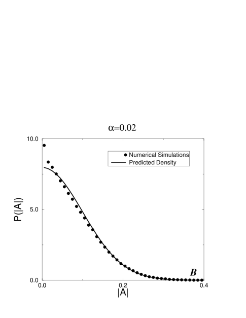
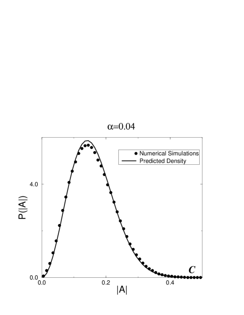
FIG. 1.: (A), (B) and (C): stationary probability densities as a function of the absolute value of $A$ for the Van der Pol-Duffing oscillator. Shown are the densities above onset for three different values of the control parameter $\alpha$. (A), $\alpha=0.015$; (B), $\alpha=0.02$; and, (C), $\alpha=0.04$. We show in (D) the bifurcation diagram showing the average value $\langle|A|\rangle$ as a function of $\alpha$. In all cases, the analytic results are represented by a solid line, whereas the symbols are the results of the numerical calculation.

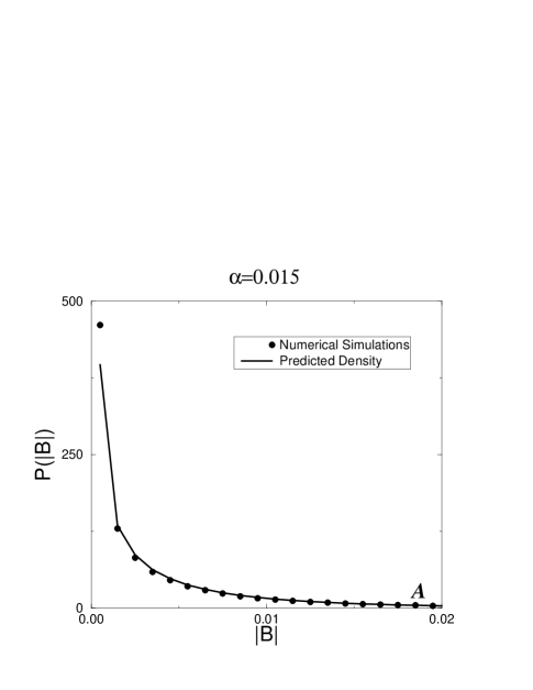
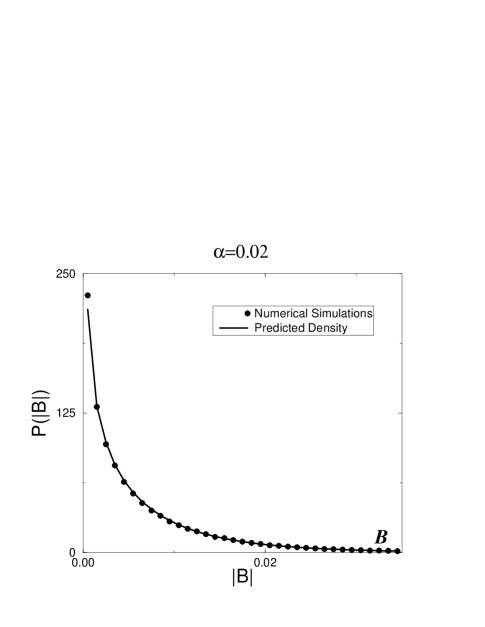
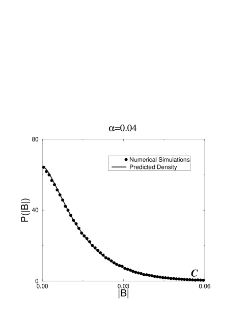
FIG. 2.: (A), (B) and (C): stationary probability densities as a function of the absolute value of $B$ for the Van der Pol-Duffing oscillator. Shown are the densities above onset for three different values of the control parameter $\alpha$. (A), $\alpha=0.015$; (B), $\alpha=0.02$; and, (C), $\alpha=0.04$. We show in (D) the bifurcation diagram showing the average value $\langle|B|\rangle$ as a function of $\alpha$. In all cases, the analytic results are represented by a solid line, whereas the symbols are the results of the numerical calculation.

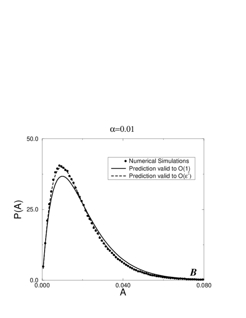
FIG. 3.: (A), (B) and (C): stationary probability densities as a function of $A$ for the transcritical bifurcation. Shown are the densities above onset for three different values of the control parameter $\alpha$. (A), $\alpha=-0.005$; (B), $\alpha=0.01$; and, (C), $\alpha=0.04$. We show in (D) the bifurcation diagram showing $\langle A\rangle$ as a function of $\alpha$. In all cases, the analytic results to ${\cal O}(1)$ and ${\cal O}(\epsilon^{2})$ are represented by solid and dashed lines respectively, whereas the symbols are the results of the numerical calculation.

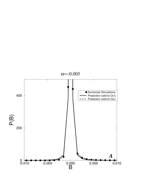
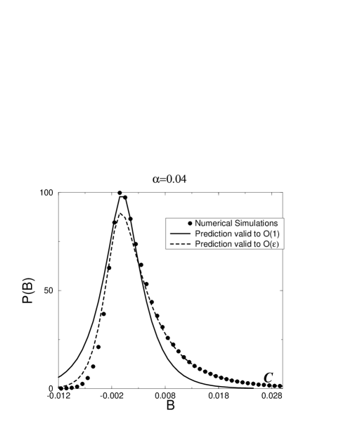
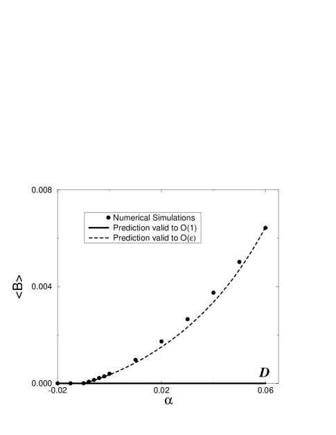
FIG. 4.: (A), (B) and (C): stationary probability densities as a function of $B$ for the transcritical bifurcation. Shown are the densities above onset for three different values of the control parameter $\alpha$. (A), $\alpha=-0.005$; (B), $\alpha=0.01$; and, (C), $\alpha=0.04$. We show in (D) the bifurcation diagram showing $\langle B\rangle$ as a function of $\alpha$. In all cases, the analytic results to ${\cal O}(1)$ and ${\cal O}(\epsilon)$ are represented by solid and dashed lines respectively, whereas the symbols are the results of the numerical calculation.