Abstract

Relativistic integral representation in terms of experimental neutron–proton scattering phase shifts alone is used to compute the charge form factor of the deuteron $G_{Cd}(Q^{2})$. The results of numerical calculations of $|G_{Cd}(Q^{2})|$ are presented in the interval of the four–momentum transfers squared $0\leq Q^{2}\leq 35\>fm^{-2}$. Zero and the prominent secondary maximum in $|G_{Cd}(Q^{2})|$ are the direct consequences of the change of sign in the experimental ${}^{3}S_{1}$– phase shifts. Till the point $Q^{2}\simeq 20\;fm^{-2}$ the total relativistic correction to $|G_{Cd}(Q^{2})|$ is positive and reaches the maximal value of 25% at $Q^{2}\simeq 14fm^{-2}$.

Deuteron is the brightest example of intersection of nuclear and particle physics. During more then sixty years it serves as source of important information about the nuclear forces, mesonic and baryonic degrees of freedoms in nuclei, relativistic effects and a possible role of quarks in nuclear structure. Therefore it is not surprising that currently the electromagnetic (EM) structure of the deuteron is a subject of intensive theoretical (the list of publication is immense) and experimental investigations.

With new experimental data from Jefferson Lab on elastic electron-deuteron scattering expected in the near future [1, 2], at momentum transfers in the GeV-range, one needs to develop relativistic approaches to the (np)-bound state problem. Recent experimental results from MIT-Bates [3] provided the first experimental evidence for a zero in the deuteron charge form factor $G_{Cd}$ at about $Q^{2}$= 20 fm^-2 predicted in a number of theoretical models (or not predicted, as in some kinds of quark models). Here we report new results of numerical calculations of $G_{Cd}$ . These calculations are based on the approach to the relativistic impulse approximation, which was briefly discussed in ref. [4] (see also the review [5] and, especially, the references herein). The more detailed formulae are contained in ref. [6]. In this approach the deuteron form factors are expressed in terms of experimental neutron–proton $(n-p)$ phase shifts in the triplet scattering channel and experimental values of nucleon EM form factors.

According to ref. [6] the formula for $G_{Cd}(Q^{2})$ appears as

$$G_{Cd}(Q^{2}) = (\rho\tilde{B}^{20}+\tilde{B}^{22})^{2}G_{Cd}^{00}(Q^{2})-$$ (1)

$$-(\rho\tilde{B}^{20}+\tilde{B}^{22})(\rho\tilde{B}^{00}+\tilde{B}^{02})[G_{Cd}^{02}(Q^{2})+G_{Cd}^{20}(Q^{2})]+$$

$$+(\rho\tilde{B}^{00}+\tilde{B}^{02})^{2}G_{Cd}^{22}(Q^{2})\;.$$

In eq.( 1) $\rho$ is the constant which describes mixing of two $n-p$ states with different orbital moments ($l=0$ and $l=2$) at the point of the bound state, i.e., the deuteron. This constant is defined by the correspondence principle. Analysing the nonrelativistic limits of eqs.(1),(2), we can prove that $\rho$ appears to be the standard asymptotic $D/S$ –ratio of the radial deuteron wave functions, so $\rho=0.0277$ (numerical calculations show that the dependence of DCFF on the variation of $\rho$ is very weak). All four elements of the matrix $\tilde{B}^{ll^{\prime}}(s)$ ($l,l^{\prime}=0,2$)  are taken at the bound state point $s=M_{d}^{2}$ ($M_{d}=2M-\varepsilon$, where $M_{d},M$ are deuteron and nucleon masses and $\varepsilon$ is the deuteron binding energy). All relativistic aspects of the two–nucleon problem are contained in $G^{ll^{\prime}}$– matrix:

$$G_{Cd}^{ll^{\prime}} = \Gamma^{2}\int_{4M^{2}}^{\infty}\frac{ds\Delta B^{\dagger}(s)}{s-M^{2}_{d}}\int_{s_{1}(s,t)}^{s_{2}(s,t)}\frac{ds^{\prime}g_{c}(s,s^{\prime}t)\Delta B(s^{\prime})}{s^{\prime}-M^{2}_{d}},$$

$$s_{2,1} = 2M^{2}+\frac{1}{2M^{2}}(2M^{2}-t)\cdot(s-2M^{2})\pm$$ (2)

$$\pm\frac{1}{2M^{2}}\sqrt{(-t)(4M^{2}-t)s(s-4M^{2})}\;.$$

In eq.(2) $\Gamma^{2}$ is the normalization constant, which is calculated from the condition $G_{Cd}(0)=1$. Matrix functions $\Delta B^{ll^{\prime}}(s)=B^{ll^{\prime}}(s+i\varepsilon)-B^{ll^{\prime}}(s-i\varepsilon)$ are the discontinuities of the Jost matrix $B(s)$. As usual, the Jost matrix is the solution of the boundary problem in two–channel scattering theory:

$$S(s)B_{+}(s) = B_{-}(s),$$

$$s \geq 4M^{2},$$ (3)

$$S(s)\equiv S\left[\delta,\eta,\varepsilon\right]=\left(\begin{array}[]{ll}\cos{2\varepsilon}\cdot e^{2i\delta}&i\sin{2\varepsilon}\cdot e^{i(\delta+\eta)}\\ i\sin{2\varepsilon}\cdot e^{i(\delta+\eta)}&\cos{2\varepsilon}\cdot e^{2i\eta}\end{array}\right)\;.$$ (4)

The reduced Jost matrix $\tilde{B}$ in eq.( 1) is the solution of the same eq.(3) with the scattering matrix $\tilde{S}\equiv S(\tilde{\delta},\tilde{\varepsilon},\tilde{\eta})$. Expressions for $\tilde{B}$ and $B$ in terms of $n-p$ phase shifts are cumbersome and are summarized in Appendix B.

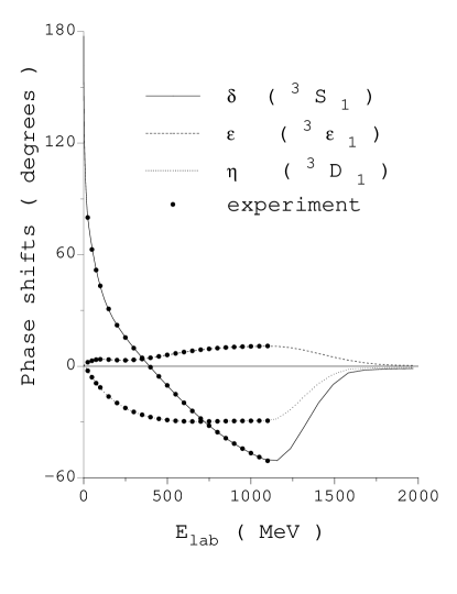
Figure 1: Neutron–proton phase shifts ${}^{3}S_{1},^{3}D_{1},^{3}\varepsilon_{1}$ used in the calculations. Experimental data are taken from the VPI analysis ref.[7].

The matrix functions $g^{ll^{\prime}}_{c}(s,s^{\prime},t)$ of three variables are the relativistic charge form factors of the unconnected part of the matrix element of EM current $\langle n^{\prime}p^{\prime}|j_{\mu}|np\rangle$. The results of the calculations of $g^{ll^{\prime}}_{c}$ are given in Appendix C. It is interesting to note that in the general case in the relativistic regime $g^{ll^{\prime}}_{c}$– functions are not factorizable in $s,s^{\prime}$ variables, whereas in the nonrelativistic limit such factorization takes place. It means that in the framework of the used relativistic approach [4]-[6] it is impossible to introduce a concept of relativistic deuteron wave function.

The experimental set of $n-p$ phase shifts were taken from the analysis of Virginia Tech group [7] and is shown in Fig. 1. This analysis was made in the energy range $0<E_{lab}\leq 1100$ MeV. Extrapolation to higher energies is not as important for the calculations of $G_{Cd}$ for the small and intermediate values of $Q^{2}$. The only essential circumstance is that ${}^{3}S_{1}$–phase shifts change sign from positive to negative and have the minimum near the energy $E_{lab}\sim 1$GeV, then go to zero in accordance with the Levinson’s theorem. Any realistic $n-p$ ${}^{3}S_{1}$ – phase shift analysis has such a behavior. Two other states (${}^{3}D_{1}$ and ${}^{3}\varepsilon_{1}$ ) give a relatively small contribution to $G_{Cd}$.

For the calculations of $G_{Cd}$ we used (as a first step) the simplest choice of the nucleon form factors: $G_{Ep}=(1+Q^{2}/18.23\;fm^{-2})^{-2},G_{Mp}/\mu_{p}=G_{Mn}/\mu_{n}=G_{Ep},\;G_{En}\equiv 0$ for all $Q^{2}$.

The result of the calculations are presented in Fig. 2. Our brief conclusions are the following.

1. The appearance of zero and secondary maximum in $|G_{Cd}(Q^{2})|$ at intermediate values of $Q^{2}$ is the direct consequence of the change of sign of the experimental ${}^{3}S_{1}$– phase shifts at intermediate energies. It is easy to calculate that the model’s $\delta(E)$, which decreases monotonically with $E$ and is always positive ($\delta(E)>0$ for all $E$), immediately leads to monotonically decreasing with $Q^{2}$ values of $|G_{Cd}(Q^{2})|$ without any fine structure.

2. Almost up to the point of zero ($Q^{2}\simeq 21\;fm^{-2})$ of $|G_{Cd}(Q^{2})|$ the total relativistic correction (TRC), i.e., the difference between $G_{Cd}$ calculated relativistically (1,2) and its nonrelativistic limit, is positive and appears to be not small. For example, for $Q^{2}\simeq 14\;fm^{-2}$ it reaches the value of 25%.

3. TRC becomes large in the region of the secondary maximum of $|G_{Cd}(Q^{2})|$, increasing the magnitude of the form factor.

4. The obtained results are consistent with the available data on $G_{Cd}$ from MIT-Bates [3]. Forthcoming data from Jefferson Lab E–94-018 [1] are extremely important to test the proposed relativistic approach in the region of higher transferred momenta, where relativistic corrections appear to be significant.

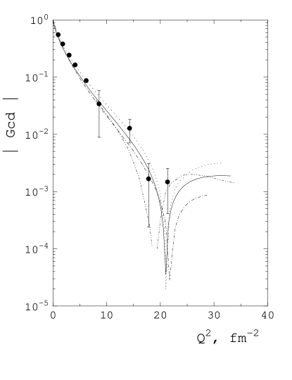
Figure 2: Relativistic deuteron charge form factor (solid line) and its nonrelativistic limit (dash-dotted line). A result with nonzero values of $G_{En}=-\mu_{n}\tau G_{Ep}$ is also shown with a short-dash line. A representative result of the relativistic approach of Arnold, Carlson,Gross [8] (dash-double-dotted line) is presented for comparison.

We would like to make the following comments to the obtained results. First, the dependence of $|G_{Cd}(Q^{2})|$ structure on the choice of different sets of experimental $n-p$ phase shifts available from the literature is strong enough. Possible variation of $\delta,\varepsilon,\eta$ may shift the position of zero in $|G_{Cd}(Q^{2})|$ from the indicated point $Q^{2}=21\;fm^{-2}$ to the point $Q^{2}=16\;fm^{-2}$ or to the point $Q^{2}=23\;fm^{-2}$. At the same time the secondary maximum is located in the interval $26\leq Q^{2}\leq 32\;fm^{-2}$, and its height may change by a factor of seven. We can see that for improving our understanding of $|G_{Cd}(Q^{2})|$ it would be desirable to obtain a more definite phase shifts analysis of $n-p$ scattering in triplet channel in intermediate energy region $E_{lab}\leq 1$ GeV. Secondly, let us indicate the dependence of $|G_{Cd}(Q^{2})|$ on the possible choice of nucleon EM form factors. Since the uncertainties of $G_{Ep}(Q^{2})$ in the considered range of $Q^{2}$ are very small, the main effect in $|G_{Cd}(Q^{2})|$ may be caused only by variation of $G_{En}(Q^{2})$. It seems to be generally accepted that the maximal deviation of $G_{En}(Q^{2})$ from the zero-value approximation $G_{En}\equiv 0$ is given by known formula $G_{En}(Q^{2})=-\mu_{n}\tau G_{Ep}(Q^{2})$, where $\mu_{n}=-1.91$ is the neutron anomalous magnetic moment and $\tau=Q^{2}/4M^{2}$. The results of the calculations of $|G_{Cd}(Q^{2})|$ with this nonzero values of $G_{En}(Q^{2})$ are shown in Fig.2. One can see that the effect is sizable and the contributions of relativistic effects and nonzero $G_{En}$ have a similar behaviour.

Finally, we show for comparison in Fig.2 the results of calculation of $G_{Cd}$ in a relativistic approach, developed in ref. [8]. It may be seen that zero of $|G_{Cd}(Q^{2})|$ predicted in ref.  [8] is shifted to the lower values of $Q^{2}$ and the height of the secondary maximum is approximately the same as in our calculations. Note that in more recent calculations in the similar approach [9] the predicted position of zero in $|G_{Cd}(Q^{2})|$ remains almost unchanged.

Here we restricted ourselves only to the discussion of the deuteron charge form factor $G_{Cd}$ . Even in this case we omitted such interesting questions as an analytical representation of relativistic corrections in different orders in $(v/c)^{2}$, the new representation for realistic deuteron wave functions, the role of relativistic rotation of nucleon spins and orbital momentum $l=2$ in the deuteron, the problem of extraction, using the present approach, of $G_{En}(Q^{2})$ for ultralow values of $Q^{2}$ from experimental data on elastic ed–scattering, and contributions from meson–exchange currents. It would also be interesting to perform a detailed comparison of the present approach with other relativistic approaches to the description of deuteron structure.

All these questions, as well as the calculations of the deuteron magnetic and quadrupole form factors will be discussed in forthcoming publications.

Acknowledgements.

A.A. would like to thank F. Gross, J.W. Van Orden and I. Strakovsky for useful discussions. The work of A.A. was supported by the US Department of Energy under contract DE–AC05–84ER40150.

Appendix A Kinematic variables.

By definition $s$ is the invariant mass of $n-p$ system squared:

$$s=(p_{n}+p_{p})^{2}_{\mu}\>.$$

In laboratory (LS) and center-of-mass (CMS) systems we have

$$s=4M^{2}+2E=4M^{2}+4p^{2}\>,$$

where $E$ is the nucleon’s energy in LS and $p$ is modulus of the nucleon 3–momentum in CMS.

$Q^{2}$ is the magnitude of the 4–momentum transfer squared:

$$Q^{2}\equiv-q^{2}_{\mu}\equiv-t>0\>.$$

Appendix B Jost matrices $B,\tilde{B}$.

The formulae for pairs ($S,B$) and ($\tilde{S},\tilde{B}$) have the most convenient form in the $p$–plane:

$$S(p)B_{+}(p)=B_{-}(p)\>,\mbox{ }-\infty<p<\infty\>,$$

where $S\equiv S[\delta(p),\eta(p),\varepsilon(p)]$, see eq.(4). Let us introduce two new matrices $\tilde{S}$ and $\tilde{B}$:

$$\begin{array}[]{rlr}\tilde{B}_{\pm}(p)&=R(\mp p)B_{\pm}(p),&\\ R(p)&=I-{2i\alpha\over(p+i\alpha)(1+\rho^{2})}\cdot\left(\begin{array}[]{lr}1&-\rho\\ -\rho&\rho^{2}\end{array}\right),&(\alpha^{2}=M\varepsilon).\end{array}$$

Now the equation for $\tilde{B}$ has the form

$$\left\{\begin{array}[]{rlr}\tilde{S(p)}\tilde{B}_{+}(p)=&\tilde{B}_{-}(p),&-\infty<p<\infty\;,\\ \tilde{S}(p)=&R(p)S(p)R^{-1}(-p)\equiv\tilde{S}[\tilde{\delta},\tilde{\eta},\tilde{\varepsilon}].&\end{array}\right.$$ (5)

The last equation defines the reduced phase shifts $\tilde{\delta},\tilde{\varepsilon},\tilde{\eta}$ as functions of input experimental phase shifts $\delta,\varepsilon,\eta$.

The solution of eq.(5) was found in ref.[10] in the form of series

$$\tilde{B}_{\pm}(p)=\tilde{B}_{\pm,0}(p)\cdot[I+\sum_{m=1}^{\infty}\tilde{B}_{\pm,m}(p)],$$

where

$$\tilde{B}_{\pm,0}(p)=\left(\begin{array}[]{lr}\varphi_{1}(p)e^{\mp\tilde{\delta}(p)}&0\\ 0&\varphi_{2}(p)e^{\mp\tilde{\eta}(p)}\end{array}\right)\>,$$

$$\varphi_{1}(p)=\exp[-\frac{1}{\pi}V.P.\int_{-\infty}^{\infty}{\tilde{\delta}(p^{\prime})dp^{\prime}\over p^{\prime}-p}],$$

$$\varphi_{2}(p)=\exp[-\frac{1}{\pi}V.P.\int_{-\infty}^{\infty}{\tilde{\eta}(p^{\prime})dp^{\prime}\over p^{\prime}-p}],$$

$$\tilde{B}_{\pm,m}(p)=\frac{1}{2\pi i}\int_{-\infty}^{\infty}{dp^{\prime}\over p-p^{\prime}\pm i0}\cdot\sum_{n=1}^{m}G_{n}(p^{\prime})\tilde{B}_{+,0}(p^{\prime})[\tilde{B}_{+,m-n}(p^{\prime})]^{1-\delta_{mn}}.$$ (6)

In eq.(6) for odd $n$

$$G_{n}(p)=i(-1)^{\frac{n-1}{2}}\cdot\frac{1}{n!}\cdot[2\tilde{\varepsilon}(p)]^{n}\cdot\left(\begin{array}[]{ll}0&e^{i(\tilde{\delta}+\tilde{\eta})}\\ e^{i(\tilde{\delta}+\tilde{\eta})}&0\end{array}\right)$$

and for even $n$

$$G_{n}(p)=i(-1)^{\frac{n}{2}}\cdot\frac{1}{n!}[2\tilde{\varepsilon}(p)]^{n}\cdot\left(\begin{array}[]{ll}e^{2i\tilde{\delta}}&0\\ 0&e^{2i\tilde{\eta}}\end{array}\right),$$

$\delta_{mn}$ is the Kroneker delta.

Appendix C $g^{ll^{\prime}}_{c}$–matrix.

In terms of invariant variables $s,s^{\prime},t$ and the nucleon EM form factors the matrix elements have the form:

$$g_{c}^{00}(s,s^{\prime},t)=$$

$$g(s,s^{\prime},t)[g_{1}(s,s^{\prime},t)(\cos\alpha_{1}\cos\alpha_{2}-\frac{1}{3}\sin\alpha_{1}\sin\alpha_{2})\cdot G_{EN}^{s}(Q^{2})+$$

$$+\frac{1}{2M}g_{2}(s,s^{\prime},t)\cdot(\frac{1}{3}\sin\alpha_{1}\cos\alpha_{2}-\cos\alpha_{1}\sin\alpha_{2})\cdot G^{s}_{MN}(Q^{2})]\;,$$

$$g_{c}^{02}(s,s^{\prime},t)=$$

$$g(s,s^{\prime},t)\{g_{1}(s,s^{\prime},t)(-\sqrt{2}P_{20}\cos\alpha_{1}\sin\alpha_{2}+\frac{1}{\sqrt{2}}P_{21}\sin\alpha_{1}\cos\alpha_{2})\cdot G^{s}_{EN}$$

$$-\frac{1}{2M}g_{2}(s,s^{\prime},t)(\sqrt{2}P_{20}\sin\alpha_{1}\cos\alpha_{2}+\frac{1}{\sqrt{2}}P_{21}\cos\alpha_{1}\sin\alpha_{2})G^{s}_{MN}\},$$

$$g_{c}^{20}(s,s^{\prime},t)=g_{c}^{02}(s^{\prime},s,t),$$

$$g_{c}^{22}(s,s^{\prime},t)=$$

$$g(s,s^{\prime},t)\Bigl{\{}g_{1}(s,s^{\prime},t)\Bigl{[}(\frac{1}{3}P_{21}P^{\prime}_{21}+\frac{2}{3}P_{20}P^{\prime}_{20})\cos(\alpha_{1}-\alpha_{2})+$$

$$+(\frac{1}{12}P_{22}P^{\prime}_{22}+\frac{1}{3}P_{20}P^{\prime}_{20})\cos\alpha_{1}\cos\alpha_{2}+$$

$$+\Bigl{(}\frac{1}{12}(P_{22}P^{\prime}_{21}-P_{21}P^{\prime}_{22})+\frac{1}{2}(P_{21}P^{\prime}_{20}-P_{20}P^{\prime}_{21})\Bigr{)}\sin(\alpha_{1}-\alpha_{2})-$$

$$-\frac{1}{6}(P_{22}P^{\prime}_{20}+P_{20}P^{\prime}_{22})\sin\alpha_{1}\sin\alpha_{2}\Bigr{]}\cdot G^{s}_{EN}-\frac{1}{2M}g_{2}(s,s^{\prime},t)\cdot$$

$$\Bigl{[}\frac{1}{12}\bigl{(}(P_{21}P^{\prime}_{22}-P_{22}P^{\prime}_{21})+\frac{1}{2}(P_{20}P^{\prime}_{21}-P_{21}P^{\prime}_{20})\bigr{)}\cdot$$

$$\cos(\alpha_{1}-\alpha_{2})-(\frac{1}{12}P_{22}P^{\prime}_{22}+\frac{1}{3}P_{20}P^{\prime}_{20})\cos\alpha_{1}\sin\alpha_{2}-$$

$$-\frac{1}{6}(P_{22}P^{\prime}_{20}-P_{20}P^{\prime}_{22})\sin\alpha_{1}\cos\alpha_{2}+$$

$$+(\frac{1}{3}P_{21}P^{\prime}_{21}+\frac{2}{3}P_{20}P^{\prime}_{20})\sin(\alpha_{1}-\alpha_{2})\Bigr{]}\cdot G^{s}_{MN}\Bigr{\}}\;,$$

where

$$\begin{array}[]{rl}g(s,s^{\prime},t)=&{g_{1}(s,s^{\prime},t)\cdot(-t)\over\sqrt{(s-4M^{2})(s^{\prime}-4M^{2})}}\cdot\frac{1}{[\lambda(s,s^{\prime},t)]^{3/2}}\cdot\frac{1}{\sqrt{1+\tau}},\\ g_{1}(s,s^{\prime},t)=&s+s^{\prime}-t,\\ g_{2}(s,s^{\prime},t)=&\Bigl{[}(-1)\bigl{(}M^{2}\lambda(s,s^{\prime},t)+ss^{\prime}t\bigl{)}\Bigr{]}^{1/2},\\ \lambda(s,s^{\prime},t)=&s^{2}+s^{\prime 2}+t^{2}-2(ss^{\prime}+st+s^{\prime}t).\end{array}$$

$P_{lm}$ are the Legendre polynomials, $P_{lm}\equiv P_{lm}(x)$ and $P^{\prime}_{lm}\equiv P_{lm}(x^{\prime})$, where

$$\begin{array}[]{rl}x(s,s^{\prime},t)=&\frac{\sqrt{s^{\prime}(s^{\prime}-s-t)}}{\sqrt{(s^{\prime}-4M^{2})\lambda(s,s^{\prime},t)}},\\ x^{\prime}(s,s^{\prime},t)=&-x(s^{\prime},s,t).\end{array}$$

The angles $\alpha_{1},\alpha_{2}$ of the relativistic rotation of nucleon spins in deuteron are

$$\begin{array}[]{ll}\alpha_{1}=&\arctan{g_{2}(s,s^{\prime},t)\over M\bigl{[}(\sqrt{s}+\sqrt{s^{\prime}})^{2}-t\bigr{]}+\sqrt{ss^{\prime}}(\sqrt{s}+\sqrt{s^{\prime}}+2M)},\\ \alpha_{2}=&\arctan{g_{2}(s,s^{\prime},t)(\sqrt{s}+\sqrt{s^{\prime}}+2M)\over M(s+s^{\prime}-t)(\sqrt{s}+\sqrt{s^{\prime}}+2M)+\sqrt{ss^{\prime}}(4M^{2}-t)}.\end{array}$$

$\tau=Q^{2}/4M^{2}$ ; $G^{s}_{E,MN}=\frac{1}{2}(G_{E,Mp}+G_{E,Mn})$ are the nucleon isoscalar charge and magnetic form factors.

References

• [1] Jefferson Lab Experiment 94-018, Measurement of the Deuteron Tensor Polarization at Large Momentum Transfers in $D(e,e^{\prime}d)$ Scattering, Spokepersons: S. Kox, E.J. Beise.
• [2] Jefferson Lab Experiment 94-018, Measurement of the Electric and Magnetic Elastic Structure Functions of the Deuteron at Large Momentum Transfers, Spokeperson: G.G. Petratos.
• [3] M. Garcon, J. Arvieux, D.H. Beck et al., Phys. Rev. C49 (1994) 2516.
• [4] V.E. Troitski, S.V. Trubnikov, I.I. Belyantsev, In: Few Body Problem in Physics, ed. by L.D. Faddeev and I.I. Kopaleishvili, World Scientific, Singapore, 1985, p.480.
• [5] V.M. Muzafarov, V.E. Troitski, S.V. Trubnikov, Sov. J. Part. Nucl.14 (5) (1983) 467.
• [6] V.A. Romanov, S.V. Trubnikov, R.L. Kostin, Bull. of the Academy of Sciences of the USSR, Phys.Ser. 53 (1989) 100.
• [7] R.A. Arndt, L.D. Roper, L.R.Workman and M.W. McNauhton, Phys. Rev. D45 (1992) 3995.
• [8] R.G. Arnold, C.E. Carlson, F. Gross, Phys. Rev. C21 (1980) 3995.
• [9] J.W. Van Orden, N. Devine, and F. Gross, Phys. Rev. Lett. 75 (1995) 4369.
• [10] V.M. Muzafarov, Theor. Math. Phys. (USSR) 58 (1984) 184.