Phase chaos in the anisotropic complex Ginzburg-Landau Equation

Abstract

Of the various interesting solutions found in the two-dimensional complex Ginzburg-Landau equation for anisotropic systems, the phase-chaotic states show particularly novel features. They exist in a broader parameter range than in the isotropic case, and often even broader than in one dimension. They typically represent the global attractor of the system. There exist two variants of phase chaos: a quasi-one dimensional and a two-dimensional solution. The transition to defect chaos is of intermittent type.

The complex Ginzburg-Landau equation (CGLE) plays the role of a generalized normal form for spatially extended media in the vicinity of a supercritical Hopf bifurcation involving a non-degenerate (oscillatory) mode. It has a wide range of applications extending from hydrodynamic instabilities [1, 2] and nonlinear optics [3] to oscillatory chemical instabilities like the Belousov-Zhabotinsky reaction [4] or oxidation on catalytic surfaces [5]. For a general review see e.g [6].

The one-dimensional (1D) and the 2D isotropic cases have been investigated rather well [7]-[16]. A number of results have also been obtained in 3D [17, 18]. Taking up some earlier work [19] we recently reported about spirals and ordered defect chains in the anisotropic complex Ginzburg-Landau equation(ACGLE) [20]

$$\partial_{t}A=[1+(1+ib_{1})\partial_{x}^{2}+(1+ib_{2})\partial_{y}^{2}-(1+ic)|A|^{2}]A.$$ (1)

Here $A$ is the complex amplitude modulating the critical mode in space and time. The usual reduced units are used. This equation was also studied in the context of defect chaos (DC) [21] and wind-driven Eckmann boundary layers [22].

Actually the range of applicability of Eq. (1) is considerable. The isotropic case, i.e. Eq.(1) with $b_{1}=b_{2}=b$, can essentially be applied only to isotropic systems undergoing a spatially homogeneous Hopf bifurcation. A nonzero wavenumber $q_{c}$ leads to traveling or standing waves, as in many hydrodynamic instabilities. Then, in systems that are isotropic in the basic state, one has a continuous degeneracy of the critical modes, which makes a more elaborate description necessary. In the presence of an anisotropy, like e.g. in the well-studied system of electro-convection in liquid crystals [2], this degeneracy is typically lifted and Eq.(1) is appropriate. Also, of course, anisotropic systems with a $q_{c}=0$ bifurcation, as occur in oscillatory surface reactions [5], require $b_{1}\neq b_{2}$. Taking linear transformations of $x$ and $y$ into account the term involving second derivatives is general. Transforming into a co-moving frame a linear group velocity involving a first space derivative vanishes. In the (common) situation of degeneracy between left- or right-traveling waves, we assume only one type to survive (which is often the case).

The ACGLE has a 2D wave-vector band of plane-wave solutions $A=F\times\exp{i(Qx+Py-\omega t)},\,F^{2}=1-Q^{2}-P^{2},\,\omega=c+(b_{1}-c)Q^{2}+(b_{2}-c)P^{2}$. They are stable against long-wavelength modulations when $(1+2\frac{1+c^{2}}{1+b_{1}c})Q^{2}+(1+2\frac{1+c^{2}}{1+b_{2}c})P^{2}<1$ holds (generalized Eckhaus instability) while the Newell criterion

$$1+b_{i}c>0,\quad i=1,2$$ (2)

is satisfied in both directions. From these relations one sees that the stable $Q$ band shrinks to zero as $1+b_{1}c\to 0^{+}$ (Benjamin-Feir (BF) instability) with a similar behavior of the $P$ band. Actually, the Eckhaus instability for $(Q,P)\neq 0$ is of the convective type and plane waves can occur over a limited spatial extension in a larger range [10].

The bifurcation connected with this instability is supercritical when one is at the BF limit or sufficiently near to it, i.e the amplitude of the destabilizing side-band modes actually saturates [23]. However, the resulting quasi-periodic solutions, as far as they are themselves modulationally stable, have for vanishing $(Q,P)$ a small basin of attraction in the BF unstable range, and in the studied 1D and isotropic cases the relevant attractors turn out to be spatio-temporally chaotic. Nevertheless, since the amplitude $|A|$ saturates to a value near 1, only the phase $\Phi$ (we write $A=|A|\exp{i\Phi}$) is dynamically active. In 1D the bifurcation at the BF instability, including slow modulations, is captured by the celebrated Kuramoto-Sivashinsky phase equation (see below). It exhibits the so-called phase chaos (PC) (or phase turbulence).

PC in the 1D CGLE was studied numerically first by Sakaguchi [24], who also studied the breakdown and crossover to chaos involving phase slips (zeros of $A$ in space-time) further away from the BF curve. This state is, in analogy to the 2D case (see below), often referred to as defect turbulence or defect chaos (DC) [7]. The resulting phase diagram was studied numerically in detail by Shraiman et al. [25], who discovered that for $|b|\geq 1.8$ the transition between PC and DC is continuous, whereas it is hysteretic with a bi-chaotic region otherwise (see Fig. 1, dashed-dotted line and region marked bichaos 1D). A detailed study with longer simulations and larger systems was performed by Egolf and Greenside [26].

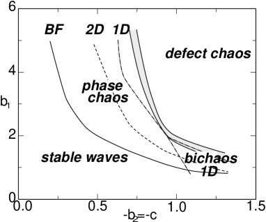
FIG. 1.: phase diagram for $b_{2}=c$

A rather exhaustive study in 2D (isotropic case $b_{1}=b_{2}$) was presented by Manneville and Chaté [27]. Here the region of PC is somewhat smaller than in 1D (see Fig. 1, broken line). Also, the transition is always hysteretic, which may be related to the fact that the zeros of $A$ now correspond to topological defects. The breakdown of PC involves the creation of pairs of defects of opposite polarity which separate and loose correlation (”unbind”). Once initiated, the process is self sustaining leading to a nucleus and eventually to fronts that appear always to invade the PC state [27]. Thus in the isotropic case PC is never the globally stable attractor.

Actually over much of the region where one has PC the global attractor is not DC as such, which appears only transiently, but rather a frozen state (vortex glass) with a disordered distribution of defects [9, 12, 27]. Every second defect emits a spiral wave of the type well known in the Eckhaus-stable range. The emitted waves remain intact over finite-sized cells by convective stabilization. Rotating spirals (time dependence $\propto\exp{i\omega t}$) exist also in the ACGLE. In spirals the group velocity, which in plane waves is $2(b_{1}-c)q$ in the $x$ direction [$2(b_{2}-c)p$ in the $y$ direction] is expected to point outward in all directions. In order to have coherent wavefronts one needs $(b_{1}-c)(b_{2}-c)>0$. Our simulations confirm that spirals are found only under this condition. Also the expected aspect ratio $\sqrt{(b_{1}-c)/(b_{2}-c)}$ of the equiphase lines of spirals is confirmed by the simulations.

Our investigation was motivated in particular by the question of what happens in the parameter regime $(b_{1}-c)(b_{2}-c)<0$ where spirals do not exist, and therefore also the existence of DC could be questionable. With this inequality the BF instability (necessary for PC) can only occur in one direction (we choose $b_{1}c<-1$, i.e. instability in the x direction) and the anisotropy is ”strong” [28]. Since the ACGLE has the symmetry $(b_{1},b_{2},c,A)\to(-b_{1},-b_{2},-c,A^{*})$, we always chose $b_{1}>0$ (in comparing with other works we transformed to this convention), and therefore $b_{1}-c>0$.

The quick answer to the above question is actually quite simple: The system remains in PC ”longer” than in the isotropic case, but eventually it does develop (”anisotropic”) DC. Since in DC defects actually hardly emit waves, in contrast to the situation in the vortex glass, no problem arises with opposite group velocities. The investigation led to surprises to be discussed now.

We have performed detailed simulations of the ACGLE in systems of size $L$ between 100 and 2500 dimension-less units with discretization $\triangle t\approx 0.1$ and $\triangle x=L/N$ between 0.3 and 5, where $N$ is the number of Fourier modes in each direction of the pseudo-spectral algorithm used. We used periodic boundary conditions with initial conditions that imposed a zero phase difference across the system. Hence PC with a nonzero background wave-vector as studied recently in 1D [14] was excluded. The results depend only weakly on the discretization and on system size (for sufficiently large systems). Choosing $b_{1}=b_{2}$ the results of [27] could be reproduced. Subsequently we changed $b_{2}$ in the direction of $c$. This always increased the range of PC (i.e. $|c|$ could be chosen larger). The limit of PC for the case $b_{2}=c$ is depicted in Fig. 1. To the left of the shaded region no defects were observed, to the right of it DC was found. The shaded region itself is the parameter range where we found intermittency (see below). Note that for $b_{1}>2$ even the 1D limit of PC could be exceeded. Since it turns out that for the effect on PC the sign of $b_{2}-c$ is, after all, not decisive, we in fact did many of the studies at $b_{2}=c\quad(<0)$. A snapshot of the PC found there is shown in Fig. 2a.

 

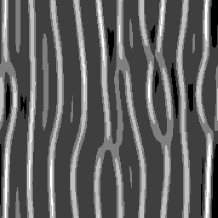
FIG. 2.: Modulus $|A|$ for $b_{1}=5.0$, $b_{2}=c=-0.25$, and system size $L=700$ (white: $|A|=1$, black: $|A|\approx 0.9).a):$ 2D PC (”PCII”) b): quasi-1D PC (”PCI”).

We now come to the qualitative new features of anisotropic PC as extracted from our simulations performed in the range $1\leq b_{1}\leq 5$ and $b_{2}=c$:

(i) PC is the global attractor, i.e. with random initial conditions the system ends up in PC after the eventual annihilation of transient defects. This is in contrast to the isotropic case, where PC is never the global attractor.

(ii) In the whole investigated range the transition between PC and DC (as $b_{2}=c$ is varied) goes through a stage of intermittency (Fig. 1 shaded region), which is not found in the isotropic case. In the intermittent state defect pairs are created in the form of bursts which subsequently annihilate again, keeping the correlation between partners, i.e. defect pairs remain bounded. So in this regime, in spite of the presence of defects, phase coherence persists and the state should therefore be classified as PC. At a critical value of $|c|$ ($=c_{u}$) defects start to unbind rather fast, and this should be associated with the onset of DC. Recently a transition between two defect chaotic states in coupled Ginzburg-Landau equations was reported where one also sees this unbinding of pairs [29].

In PC the spatial average of the amplitude $\overline{|A|}$ is very close to $1$, see Fig. 3a (solid line). One finds a kink at the onset of intermittency from where on $\overline{|A|}$ starts to drop faster. The limit of existence of PC can here be assigned to $|c|$ slightly below $0.8$. Also shown in Fig. 3a is the minimum $|A|_{min}$ of $|A|$ (broken line). Once $|A|$ falls below $|A|=0.6$ breakthrough to $A=0$ typically occurs. Figure 3b shows $|A|_{min}$ as a function of time in the intermittent range.

FIG. 3.: a): $\overline{|A|}$ (solid line) and $|A|_{min}$ (broken line) decrease with growing $|b_{2}|=|c|$ ($L=700,\ b_{1}=4.0$). b): time series of $|A|_{min}$ for $b_{1}=2.0,\,b_{2}=c=-0.96$

(iii) In addition to the 2D PC discussed up to now (”PCII”) there exists close to the BF boundary and coexistent with PCII a strictly quasi-1D PC (”PCI”) with spatial variations only in the unstable $x$ direction (see Fig. 2b for a snapshot). It is obtained by initializing the system with a function $A$ that differs from $1$ only by small variations in $x$. PCI is only stable against small perturbations in the $y$ direction and easily transforms into PCII (it is metastable). At its limit of stability, which for $b_{1}=5.0$ is slightly below $|c|=0.3(=|b_{2}|)$, the transformation becomes spontaneous [30]. Because of CPU time limitations the transition could not be studied extensively.

Next we introduce a nonlinear phase equation which should yield a simplified description of phase chaos becoming exact in the limit $1+b_{1}c\to 0^{-}$. Using the standard procedure [6] one arrives at the following equation for the (strongly) anisotropic situation

$$\partial_{t}\Phi=-|D_{x}|\partial_{x}^{2}\Phi-D_{x4}\partial_{x}^{4}\Phi-g_{x}(\partial_{x}\Phi)^{2}+D_{y}\partial_{y}^{2}\Phi-$$ (3)

$$g_{y}(\partial_{y}\Phi)^{2}-a\big{[}2\partial_{x}\Phi\partial_{x}^{3}\Phi+(\partial_{x}^{2}\Phi)^{2}+\frac{2}{b_{1}}(\partial_{x}\Phi)^{2}\partial_{x}^{2}\Phi\big{]},$$ (4)

$$D_{x}=1+b_{1}c,\quad D_{y}=1+b_{2}c,\quad D_{x4}=b_{1}^{2}(1+c^{2}),$$ (5)

$$g_{x}=b_{1}-c,\quad g_{y}=b_{2}-c,\quad a=b_{1}(1+c^{2}).$$ (6)

The first three terms on the r.h.s. of Eq. (3) make up the 1D Kuramoto-Sivashinski equation. The higher-order nonlinear terms proportional to $a$ were included by Sakaguchi, who showed them to be responsible for the breakdown of PC, here implied by a blow up of the phase gradient [24]. Actually the last term in square brackets is formally of higher order than the others, but it could become important for small $b_{1}$. In the stable $y$ direction ($D_{y}>0!$) it suffices to include the two terms shown, as done by Bar in the equation without the Sakaguchi terms [31]. Actually, in the parameter range studied by us, the term proportional to $g_{y}$ has little influence (for $b_{2}=c$ it vanishes anyhow).

By rescaling $t,x,y$, and $\Phi$ one can scale the coefficients of the linear part and the term proportional to $g_{x}$ to $1$. Introducing the time scale $\tau=D_{x4}/|D_{x}|^{2}$, the length scales become $l_{x}=\sqrt{D_{x4}/|D_{x}|}$ and $l_{y}=\sqrt{D_{y}D_{x4}}/|D_{x}|$, which is supported by the simulations of PCII. Note that when the BF boundary is approached, where $D_{x}\to 0$, $l_{y}$ diverges more rapidly than $l_{x}$, so that PCII appears more and more one dimensional. Neglecting in Eq. (3) the last term in square brackets the only relevant parameter is the prefactor of the Sakaguchi terms, which becomes ${\hat{a}}=a|D_{x}|/(D_{x4}g_{x})$.

Comparing PCII obtained from simulations of Eq. (3) with that of the ACGLE we find satisfactory agreement except near to the breakdown (for not too large values of $b_{1}$). For $b_{1}=2.0$ and $b_{2}=c$ we find the breakdown of the phase description at $b_{2}=-0.95$ which is in fair agreement with the value found for the ACGLE. In a detailed study of the 1D case at $b_{1}=3.5$ [26] the authors found $c_{1d}=-0.75$ in the CGLE and $-0.55$ in the Sakaguchi equation, whereas we find $c_{2d}=-0.9$ in the ACGLE (with $b_{2}=c$) compared to $-0.75$ with Eq. (3). PCI is also found in the phase equation and can at $b_{1}=5.0$ be maintained stably up to at least $c=-0.28$. The lowest-order description by Eq. (3) with only the first four terms on the r.h.s. has PCI and PCII as coexisting solutions.

How can one understand the existence of PCI? For a stable 1D solution, i.e. a solution with negative Lyapunov exponents, the (stable) existence of its quasi-1D analog is clear in the situation of a stable $y$ direction (this is most easily seen in the phase equation). On the other hand, in PCI one has positive Lyapunov exponents for fluctuations that vary only in the $x$ direction, so there are also positive Lyapunov exponents for sufficiently small modulation wavenumber $p$ in the $y$ direction. However, this does not necessarily destroy PCI, since the only condition is that fluctuations flatten out in $y$, even though they do not decay. We have confirmed by extensive simulations of PCI at $b_{1}=5.0,\ b_{2}=c=-0.26,L=700,$ and $N=256$ that small perturbations of the form $a_{p}\exp{ipy}$ with $a_{p}<0.2$ (at $p\approx 0.1$) decay asymptotically in a diffusive manner with a phase diffusion constant around $D_{y}$. Under the same conditions stochastic perturbations (uncorrelated on the discretized lattice in real space) decayed up to an amplitude $a_{d}<0.01$. Actually, one also expects solutions of Eq. (1) of the form $A=\exp{(iPy)}B(x,t)$ with phase-chaotic $B$ to exist. Thus PCI presumably represents the center of a $P$ band of phase-winding solutions.

Finally we point out that the interpretation of the PCII $\leftrightarrow$ DC transition as a vortex binding-unbinding transition probably allows to establish PCII as a thermodynamic phase that is qualitatively different from DC. In PCII, even if a defect pair is created, it remains bounded and annihilates again (the unbinding beyond $c_{u}$ is a cooperative phenomenon). The question of the conventional forms of PC representing such a state – in contrast to being just a (sometimes metastable) variant of DC with a very low rate of phase slips or defect pair creation – has indeed stimulated much of the previous research on PC [25, 26, 27]. Actually also PCI, although it appears to exist only metastably, can presumably be considered an independent thermodynamic phase because it differs in symmetry.

Clearly much remains to be done. On one hand, finding criteria for the occurrence of PCI and methods to calculate the boundary of existence seems a most interesting problem. On the other hand, a detailed characterization of the PCII $\leftrightarrow$ DC transition appears desirable.

We have benefitted from discussions with I. Aronson, J. Neubauer, W. Pesch, and A. Rossberg. Extensive use of high-performance computer facilities at the LRZ München (Cray T90) and the HLRS Stuttgart (NEC SX4), as well as financial support by DFG (Kr690/4) are gratefully acknowledged.

REFERENCES

- [1] W. Schöpf and W. Zimmermann, Phys. Rev. E47, 1739 (1993).
- [2] M. Treiber, and L. Kramer, Coupled complex Ginzburg-Landau equations for the weak electrolyte model of electroconvection, preprint (1997).
- [3] P. Coullet, L. Gil, and P. Rocca, Optics Comm. 73, 403 (1989); A.C. Newell and J.V. Moloney, Nonlinear optics (Addison-Wesley, 1992).
- [4] F. Hynne, P. Graae Sørenson, and T. Møller, J. Chem. Phys. 98, 219 (1993).
- [5] M. Baer, M. Hildebrand, M. Eiswirth, M. Falcke, H. Engel, and M. Neufeld, Chaos 4, 499 (1994).
- [6] M.C. Cross, and P.C. Hohenberg, Rev. Mod. Phys. 65, 851 (1993).
- [7] P. Coullet, J. Lega, and L. Gil, Phys. Rev. Lett. 62, 1619 (1989).
- [8] W.v. Saarloos and P.C. Hohenberg, Physica D56,303 (1992).
- [9] G. Huber, P. Alstrøm, and T. Bohr, Phys. Rev. Lett. 69, 2380 (1992).
- [10] I. Aranson, L. Aranson, L. Kramer, and A. Weber, Phys. Rev. A46, 2992 (1992); Physica D61, 279 (1992).
- [11] I. Aranson, L. Kramer, and A. Weber, Phys. Rev. Lett. 72, 2316 (1994); S. Popp, O. Stiller, I.S. Aranson, and L. Kramer, Physica D87, 398 (1995).
- [12] G. Huber, in Spatio-Temporal Patterns in Nonequilibrium Complex Systems, P. E. Cladis and P. Palffy-Muhoray, eds., SFI Studies in the Sciences of Complexity, Addison-Wesley, Reading MA 1995, p. 51.
- [13] H. Chaté, and P. Manneville, Physica A224,348 (1996).
- [14] R. Montagne, E. Hernández-García, and M. San Miguel, Phys. Rev. Lett. 77, 267 (1996); A. Torcini, Phys. Rev. Lett. 77, 1097 (1996).
- [15] T. Bohr, G. Huber, and E.Ott, Physica D106, 95 (1997).
- [16] M. van Hecke, Phys. Rev. Lett. 80,1896 (1998).
- [17] I. Aranson, and A. Bishop, Phys. Rev. Lett. 79, 4174 (1997).
- [18] M. Gabbay, P. Ott, and E. Guzdar Phys. Rev. Lett. 78, 2012 (1997).
- [19] A. Weber, E. Bodenschatz, and L. Kramer, Advanced Materials 3, 191 (1991).
- [20] R. Faller and L. Kramer, Chaos, Solitons and Fractals, in press.
- [21] B. W. Roberts, E. Bodenschatz, and J. P. Sethna, Physica D 99, 252 (1996).
- [22] T. M. Haeusser, and S. Leibovich, Phys. Rev. Lett. 79, 329 (1997).
- [23] B. Janiaud, A. Pumir, D. Bensimon, V. Croquette, H. Richter, and L. Kramer, Physica D 55, 269 (1992).
- [24] H. Sakaguchi, Prog. Theor. Phys. 84,792(1990).
- [25] B. I. Shraiman, A. Pumir, W. v. Saarlos, P. C. Hohenberg, H. Chaté, and M. Holen Physica D57, 241 (1992).
- [26] D. A. Egolf, and H. S. Greenside, Phys. Rev. Lett. 74, 1751 (1995).
- [27] P. Manneville, and H. Chaté, Physica D96, 30 (1996).
- [28] We have not studied the effect of small anisotropy () on PT in any detail. On first sight the simulational results appear similar to those of the isotropic case
- [29] G. D. Granzow, and H. Riecke, Physica A249, 27 (1998).
- [30] There is a small jump in from about to about (at ) at the crossover from PCI to PCII which would not be seen in Fig. 3a.
- [31] D. E. Bar doctoral thesis, Technion Haifa, 1996.