Self-consistent theory of large amplitude collective motion: Applications to approximate quantization of non-separable systems and to nuclear physics

Abstract

The goal of the present account is to review our efforts to obtain and apply a “collective” Hamiltonian for a few, approximately decoupled, adiabatic degrees of freedom, starting from a Hamiltonian system with more or many more degrees of freedom. The approach is based on an analysis of the classical limit of quantum-mechanical problems. Initially, we study the classical problem within the framework of Hamiltonian dynamics and derive a fully self-consistent theory of large amplitude collective motion with small velocities. We derive a measure for the quality of decoupling of the collective degree of freedom. We show for several simple examples, where the classical limit is obvious, that when decoupling is good, a quantization of the collective Hamiltonian leads to accurate descriptions of the low energy properties of the systems studied. In nuclear physics problems we construct the classical Hamiltonian by means of time-dependent mean-field theory, and we transcribe our formalism to this case. We report studies of a model for monopole vibrations, of ²⁸Si with a realistic interaction, several qualitative models of heavier nuclei, and preliminary results for a more realistic approach to heavy nuclei. Other topics included are a nuclear Born-Oppenheimer approximation for an ab initio quantum theory and a theory of the transfer of energy between collective and non-collective degrees of freedom when the decoupling is not exact. The explicit account is based on the work of the authors, but a thorough survey of other work is included.

PACS number(s): 21.60.-n, 21.60.Jz, 21.60.Ev

Keywords: Collective motion; Nuclear collectivity; Large amplitude collective motion; Self-consistent theory; Non-linear methods; Quantization non-separable systems.

Contents

toc

I Introduction

A Why was this review written?

The account that follows is a review of work that was stimulated by a search for a solution to the following problem: We are given a non-relativistic nuclear many-body Hamiltonian. We assume that the chosen Hamiltonian is capable of describing the low-energy properties of medium to heavy nuclei. We then set ourselves the task of deriving from this Hamiltonian a description of large amplitude collective motion (defined below) without the intervention of any additional ad hoc elements. It turns out that the solution developed for this problem has additional applications to molecular structure and reactions, to the general problem of the approximate quantization of non-separable systems, and to field theories with soliton solutions. We shall also include examples of these additional applications in the following review, except for the soliton problem, which would take us too far afield.

For nuclear physics, the “simplest” applications of such a theory are to the rotational-vibrational motion of deformed nuclei and to fission, though applications to reaction and transport processes are also of great interest. Historically, it was the first of the problems cited that called attention to the need for a deeper theory than the one that was first applied (successfully) to its solution. We refer here to the work of Kumar and Baranger [1, 2, 3, 4, 5], that we judge to be the first successful calculations, starting from a many-body Hamiltonian, of the low-energy rotations and quadrupole vibrations of deformed nuclei. The main features of this work are:

1. The stable equilibrium shape and the energy of a deformed nucleus are given by a Hartree-Bogoliubov mean-field calculation.

2. The potential energy for non-equilibrium shapes is obtained by solving a constrained Hartree-Bogoliubov problem, the constraining operator chosen plausibly as the (mass) quadrupole moment operator of the model. This calculation is not restricted to small values of the quadrupole distortion. This plus the fact that the procedure “decouples” the quadrupole degree of freedom, a collective operator depending on all the coordinates of the nucleus, from the many-body Hamiltonian accounts for the name large amplitude collective motion.

3. To complete the derivation of a model Hamiltonian, one also needs a kinetic energy. In the adiabatic (small velocity) approximation, to which this approach is limited, this means an expression quadratic in the velocities. The mass coefficients, which can also be rather general functions of the collective coordinates, are computed by the cranking method [6].

4. The classical Hamiltonian thus obtained is quantized (a not ambiguity-free procedure) and the associated Schrödinger equation solved for various medium to heavy nuclei. Results are compared to the spectroscopic data.

The method of Kumar and Baranger, with improved Hamiltonians and improved numerical algorithms, has continued to be used up to the present, for instance in the analysis of the fission process [7]. What then is “wrong” with this method? The glaring fault is that the potential energy of the nucleus is determined from a constrained search for a minimum of the mean-field energy, with a constraining operator that is an ad hoc choice. Baranger and others (Ref. [8] and the literature cited in Sec. VII) realized that it would be of interest to construct a theory of large amplitude collective motion free of this ad hoc feature. In short, the nucleus should decide internally, on the basis of the given microscopic Hamiltonian, how to deform itself, rather than have this property imposed from the outside. We refer to a formulation with this property as a self-consistent theory of large amplitude collective motion.

We restrict the account that follows largely to the solution of this problem developed by the writers and their collaborators [9, 10, 11, 12, 13, 14, 15, 16, 17, 18, 19, 20, 21, 22, 23, 24, 25, 26, 27, 28, 29, 30, 31, 32, 33, 34, 35, 36, 37, 38, 39, 40, 41]. Since we entered the arena only after a full decade of effort by others, this decision requires justification. We shall, however, postpone a detailed account of this early work, as well as other contemporaneous work until Sec. VII, i.e., until after we finish the exposition of our work. Such a review may then be more meaningful to the reader. We certainly benefited from some of this earlier research, as we shall try to make clear at appropriate junctures. Nevertheless, it is our judgment that compared to the existing literature, for the problem as we have defined it, our method is simpler in concept and more complete in execution than can be found elsewhere. This makes it suitable for a coherent account, designed to explain the basic ideas of the subject.

In addition to developing a complete theory, we have also carried out a number of applications, of which the most important are included in this account. Though we hope that the reader will be impressed by the theoretical structure and by some of the new applications, it is also true, unfortunately, that so far we have not gotten back to the applications that stimulated this research in the first place. However, a new effort in this direction has been undertaken [40, 41].

B Elementary physical considerations concerning decoupled motion

When we enter the main text, it will be easy at times to lose sight of the simple physical ideas that underlie the whole development. We shall therefore present those ideas here in an irreducibly simple setting. In the following we shall, using elementary examples, distinguish three kinds of motion, exactly separable motion (which is a fortiori decoupled), exactly decoupled motion that does not correspond to a separable Hamiltonian, and approximately decoupled motion.

We first consider the separable Hamiltonian

$$H = H_{1}(q_{1},p_{1})+H_{2}(q_{2},p_{2}),$$ (1)

$$H_{i} = \frac{1}{2}(p_{i}^{2}+\omega_{i}^{2}q_{i}^{2})+\frac{1}{4}\lambda_{i}q_{i}^{4}.$$ (2)

Classically this separable Hamiltonian allows decoupled motion in the following sense. Consider the equations of motion

$$\ddot{q}_{i}=-\omega_{i}^{2}q_{i}-\lambda_{i}q_{i}^{3}.$$ (3)

These admit, for example, the class of solutions $q_{2}(t)=0$ for the initial conditions $q_{2}(0)=\dot{q}_{2}(0)=0$. The motions $q_{1}=q_{1}(t)$ for these initial conditions then define a one-dimensional decoupled manifold. This motion is along the valley $q_{2}=0$ of the two-dimensional potential energy surface. (The precise definition of a valley will be given below.)

There is also a decoupled solution with indices 1 and 2 interchanged. However, we restrict our attention to low-energy motion and assume (adiabatic approximation) $\omega_{2}^{2}\gg\omega_{1}^{2}$, a condition whose implications we assume not to be invalidated by the quartic coupling. As a consequence of these assumptions, the “high-energy” decoupled manifold will be of no primary interest in any of the following discussion.

We now consider the associated quantum theory. The wave functions have the form

$$\psi_{n_{1}n_{2}}=\phi_{n_{1}}(q_{1})\chi_{n_{2}}(q_{2}).$$ (4)

In the adiabatic approximation, the lowest-lying states will be a set $(n_{1},0)$, with the high frequency oscillator in its ground state ($n_{2}=0$) . If we further recall that the length $1/\sqrt{\omega_{2}}$ (in suitable units) determines the very narrow width of the function $\chi_{0}(q_{2})$, we see that for this low-energy spectrum, the wave-functions are almost one-dimensional. This corresponds to the classical notion of a one-dimensional decoupled manifold. As far as energy differences are concerned, it suffices to quantize the Hamiltonian $H_{1}$ of the decoupled manifold, as long as we do not excite the second degree of freedom.

A further remark about this trivial example is that classically, small perturbations of the motion away from the decoupled manifold are stable in the sense that the fluctuations remain small in the course of time. This also reflects itself in the quantum theory in that the corresponding low-lying excited states remain well-localized in the $q_{2}$ direction.

Next we consider a slightly more complicated case where the Hamiltonian is non-separable, but the system still admits exactly decoupled motion. To the previous Hamiltonian, we now add the term

$$\delta_{1}H=\frac{1}{2}\lambda_{12}q_{1}^{2}q_{2}^{2},$$ (5)

($\lambda_{12}$ positive) leading to the equations of motion

$$\ddot{q}_{1} = -\omega_{1}^{2}q_{1}-\lambda_{1}q_{1}^{3}-\lambda_{12}q_{1}q_{2}^{2},$$ (6)

$$\ddot{q}_{2} = -\omega_{2}^{2}q_{2}-\lambda_{2}q_{2}^{3}-\lambda_{12}q_{2}q_{1}^{2}.$$ (7)

Note that these equations still admit the solution $q_{2}(t)=0$ for the initial conditions $q_{2}(0)=\dot{q}_{2}(0)=0$. Just as in the separable case, the motion takes place along a valley of the potential energy surface, as discussed further below.

For small $q_{2}\neq 0$, the equation of motion in the $q_{2}$ direction may be written (ignoring the cubic term)

$$\ddot{q}_{2} = -\Omega_{2}^{2}(q_{1})q_{2},\;\;\Omega_{2}^{2}(q_{1})=\omega_{2}^{2}+\lambda_{12}q_{1}^{2}.$$ (8)

This may be viewed as the equation of motion for an harmonic oscillator with a slowly varying (local) frequency, since the $q_{1}$ motion is supposed to be slow compared to the $q_{2}$ motion. We still expect stability with respect to small excursions away from the collective manifold.

Intuitively we still expect the eigenfunctions for the low-energy states of the quantized system to be approximately one dimensional. What shall we take as the approximate quantum Hamiltonian of such a state? The first answer is that we quantize the Hamiltonian that describes the motion on the decoupled manifold, namely $H_{1}(p_{1},q_{1})$, just as in the separable case. An improvement, that will be necessary for some of the applications to be presented in the main text, is to include the quantum corrections due to the zero point oscillations associated with the $q_{2}$ motion. For the separable case we obtain just an additive constant. For the approximation described by Eq. (8), on the other hand, the zero-point energy is $(1/2)\Omega_{2}(q_{1})$, which thus modifies the potential energy of the effective one-dimensional Hamiltonian.

Before going on to the third example, where one has neither a separable Hamiltonian nor an exactly decoupled manifold, but where one would like to explore the concept of an approximately decoupled motion, let us consider more precisely what is meant by a valley. We have used this term twice to characterize the decoupled manifolds previously identified. We wish to present a precise definition of this concept for the following reason: For the first two cases the decoupled manifold was a valley, a result that will later prove to be general. Even where there is no exactly decoupled manifold, for all examples of interest to us there will nevertheless be a valley, or its multi-dimensional generalization, that we shall put forward as the domain on which there may be approximately decoupled motion. It is therefore of interest to learn how to recognize and extract analytically such a domain, i.e., formalize our intuitive understanding of the concept.

Consider a two-dimensional potential energy surface $V(q_{1},q_{2})$ and an equipotential curve $V=\text{constant}$. We move along this curve, at each point take a step of fixed length orthogonal to the curve, and then measure the magnitude of the gradient of the potential. A local minimum for this gradient is called an element of a valley, and a local maximum an element of a ridge. For example, for the separable potential considered above, the line $q_{2}=0$, the decoupled manifold chosen, is a valley, and the line $q_{1}=0$ is a ridge. This will be shown analytically below.

The definition of the valley (or ridge) given above can be formalized as the solution of the constrained variational problem,

$$\delta[(\nabla V)^{2}-\Lambda V]=0,$$ (9)

namely, we seek stationary values of the square of the gradient of the potential (square chosen for analytical convenience) for fixed values of the potential ($\Lambda$ is a Lagrange multiplier).

We study Eq. (9) for the potential

$$V(q_{1},q_{2})=\frac{1}{2}(\omega_{1}^{2}q_{1}^{2}+\omega_{2}^{2}q_{2}^{2}+\lambda_{12}q_{1}^{2}q_{2}^{2}).$$ (10)

and derive the equations

$$[F_{1}(q_{1},q_{2})-\Lambda\Omega_{1}^{2}(q_{2})]q_{1} = 0,$$ (11)

$${}[F_{2}(q_{1},q_{2})-\Lambda\Omega_{2}^{2}(q_{1})]q_{2} = 0,$$ (12)

where it is of no particular interest to record the detailed forms of $F_{i}$ and $\Omega_{i}^{2}$. It suffices to observe that these equations have two solutions, the valley $q_{2}=0$, which satisfies Eq. (12), and the ridge $q_{1}=0$, which satisfies Eq. (11). The associated Lagrange multiplier is evaluated from the other of the pair of equations. This calculation substantiates assertions about the relationship of the chosen decoupled manifold to a valley.

As our third and last example, we consider the problem of two harmonic oscillators with the coupling term

$$\delta_{2}H=\beta q_{1}^{2}q_{2}.$$ (13)

The equations of motion

$$\ddot{q}_{1} = -\omega_{1}^{2}q_{1}-2\beta q_{1}q_{2},$$ (14)

$$\ddot{q}_{2} = -\omega_{2}^{2}q_{2}-\beta q_{1}^{2},$$ (15)

still admit one decoupled manifold, $q_{1}=0$, but this corresponds to high energy motion and is not the physics we are after. There is no decoupled motion corresponding to our previous valley $q_{2}=0$. We see this from Eq. (15); by setting $q_{2}(0)=\dot{q}_{2}(0)=0$, we obtain $\ddot{q}_{2}(0)=-\beta q_{1}^{2}(0)$.

This is an example of the general physical situation. Whereas there is no exactly decoupled manifold, what one finds in cases of interest is that there continues to be a valley, satisfying Eq. (9), where the simple valley $q_{2}=0$ is replaced by the curve

$$q_{2}=f(q_{1}).$$ (16)

We shall not present the details of the calculation of the result (16) for the example under study, since a number of such calculations will be presented in the main text. The important point is that the general theory to be developed suggests that the optimum choice of an approximately decoupled manifold is the valley (and suitable multi-dimensional generalizations) and that the appropriate classical Hamiltonian to quantize is the value of the full Hamiltonian on the valley. It follows from Eq. (16) that by applying formulas for the mass to be derived in the main text this has the form

$$2H = M(q_{1})p_{1}^{2}+\omega_{1}^{2}q_{1}^{2}+2\beta q_{1}^{2}f(q_{1}),$$ (17)

$$M(q_{1}) = \frac{1+(f^{\prime})^{2}}{(f^{\prime})^{2}},\;\;f^{\prime}=\frac{df}{dq_{1}}.$$ (18)

One can quantize Eq. (17) and as will be seen in the examples worked out in the main text, include corrections for quantum fluctuations orthogonal to the valley. (We shall not discuss here the ambiguity in the quantization of the kinetic energy.)

 

We should remark that for the specific example (14) and (15), another definition of the collective manifold suggests itself, namely, by setting the left hand side of Eq. (15) to zero, we obtain the equation

$$-\omega_{2}^{2}q_{2}=\beta q_{1}^{2}$$ (19)

as a definition of the approximately decoupled manifold. This is admittedly simpler than the exercise of computing the valley. The reason we have chosen not to pursue this suggestion is that though it may be simple to apply to systems with a few degrees of freedom, it is more difficult to systematize it for the nuclear many-body problem.

 

The review that follows consists first of the development of a theoretical framework that formalizes the (relatively) simple concepts that we have discussed above. Secondly, it reports a series of successively more elaborate applications. Following that, we turn to more fundamental questions regarding the foundations of the quantum theory of large amplitude collective motion. Finally we consider the problem of exchange of energy between the collective and the non-collective degrees of freedom in non-equilibrium processes.

II Theory of decoupling

A Formal theory of decoupled motion within a classical Hamiltonian framework

1 Introduction

In this section, we develop both a formal and several versions of a practical theory of decoupled large amplitude collective motion for Hamiltonian systems. Though our ultimate interest was in formulating such a theory for many-particle fermion systems, especially nuclei, we believe that it was an important step to divorce the considerations initially from the statistics of the particles involved and to concentrate on the Hamiltonian features of the problem. This emphasis can be found in several brief accounts in the earlier literature [42, 43]. The dominant physics of large amplitude collective motion corresponds to a well-defined classical limit of the quantum Hamiltonian. The methods and results developed in this section emerge from a Hamiltonian framework utilizing the theory of canonical transformations. In Sec. IV A we shall show how to adapt the resulting theory to the nuclear many-body problem.

Given a classical many-particle Hamiltonian, $H$, that we wish to investigate for large amplitude collective motion, the first point to recognize is that the existence of such motions may not be manifest from the given form of $H$. (This is almost universally the case for nuclear physics.) Thus the first task is to carry out a canonical transformation to a coordinate system in which the division into collective (small velocity, adiabatic) and non-collective (high velocity) coordinates can be made. The adiabatic approximation limits the generality of the transformations required, but does not restrict them to point transformations, as assumed in all work prior to ours and in our earliest work. In studying the canonical transformations and the conditions for decoupling in the general case, where the mass coefficients are functions of the coordinates, care must be taken with the tensor structure of the space. The considerations of this section is a revised (and improved) version of some of the contents of Ref. [28], which reference in turn draws from Refs. [12, 18, 22].

2 Decoupling conditions under a point transformation (adiabatic approximation)

We study a classical system with $N$ canonical pairs $\xi^{\alpha}$ and $\pi_{\alpha}$ (the “single-particle coordinates”) described by the Hamiltonian,

$$H=\frac{1}{2}\pi_{\alpha}B^{\alpha\beta}(\xi)\pi_{\beta}+V(\xi).$$ (20)

The dynamics is thus characterized by a point function $V$ and by the reciprocal mass tensor $B^{\alpha\beta}$ that also plays the role of metric tensor for the considerations that follow. (We shall sometimes omit the adjective reciprocal in future allusions to this tensor.) It is assumed that the system described by (20) admits motions that are exactly decoupled, as defined precisely below, motions that are thus fully characterized by fewer than $N$ canonical coordinates and momenta. Included in such motions are those we call collective. It is further assumed that the original coordinates are not natural ones for the description of these motions, but that a suitable set can be introduced by means of a canonical transformation. In this initial discussion, we limit ourselves to the special case of point transformations. We thus study mappings of the form

$$\xi^{\alpha}=g^{\alpha}(q^{1},...,q^{N}),$$ (21a)

with inverse

$$q^{\mu}=f^{\mu}(\xi^{1},...,\xi^{N}).$$ (21b)

The corresponding momenta are given by the formulas

$$\pi_{\alpha}=f^{\mu}_{,\alpha}p_{\mu},\;\;p_{\mu}=g^{\alpha}_{,\mu}\pi_{\alpha},$$ (22)

where the comma indicates a partial derivative. The indices $\alpha,\;\beta,...$ will enumerate the initial coordinates, and $\lambda,\;\mu,...$ the final coordinates, although each set has the same range $1,...,N$.

The point transformation (21a) is the only canonical transformation that exactly preserves the quadratic dependence on the momenta. It will be evident from the next section, however, that for small collective momenta there exists a generalization of (21a) that approximately conserves the quadratic momentum dependence. We have chosen to treat the case of point transformations separately, at least initially, because of the relative simplicity of this case, and because most (but not all) serious applications carried out up to the present are done within this framework. The restriction of the original Hamiltonian to the form (2.1) and the limitation to point transformations can justifiably be designated as an adiabatic approximation. However, this is not the most general definition of adiabatic approximation to be utilized in this review. For the latter, we start with a Hamiltonian with arbitrary dependence on its momenta, but after carrying out the canonical transformation designed to effect the decoupling, we expand the new Hamiltonian to second order in the collective momenta.

We assume that in the new coordinates we can identify a decoupled surface, defined as follows: We divide the set $q^{\mu}$ into two subsets, $q^{i},i=1...K,$ and $q^{a},a=K+1...N$, and suppose this division to be such that if at time $t=0$ both $q^{a}=0$ (by convention) and $\dot{q}^{a}=0$, then $q^{a}(t)=0$. Such motions evolve on a K-dimensional submanifold

$$\xi^{\alpha}=g^{\alpha}(q^{1}...q^{K},0,...,0)\equiv g^{\alpha}(q),$$ (23)

designated as the surface $\Sigma$. In geometrical terms, if the system point is initially on $\Sigma$, and the initial velocity is on $T\Sigma$, the tangent plane to $\Sigma$ at the given point, then provided the subsequent motion of the system is confined to this surface, $\Sigma$ is said to be decoupled. It may be useful to imagine that the system has a self-imposed set of holonomic constraints.

The main practical aim of the research that follows is to develop methods of discovering such manifolds or, more realistically, of finding manifolds that are approximately decoupled. For this enterprise, it is essential to distinguish between the totality of conditions that must be satisfied for exact decoupling to occur and the formulation of an algorithm for determining manifolds that are candidates for approximate decoupling (based on some convenient subset of this totality). Such an algorithm should then include some test of the extent of violation of the remaining conditions. The exact conditions derived below are meant to determine the functions (23), which are the defining equations of the collective submanifold and, at the same time, can be viewed as the restriction of a point canonical transformation to the surface $\Sigma$. As remarked below, they determine a dynamics on this manifold. In some cases where the decoupling is almost exact, one may consequently obtain a rather accurate description of the collective motion without having to be concerned with the non-collective coordinates. In other cases coupling to the non-collective coordinates becomes essential, and one must thus seek a full point transformation (21a), or at least extend (23) to some immediate neighborhood of the collective manifold. We shall nevertheless, in what follows immediately, restrict considerations to the collective manifold itself. The necessary extensions will be considered in Sec. II B 4.

Before deriving the conditions that characterize decoupled motion, let us note that under the point transformation (21a) and (21b), the Hamiltonian becomes

$$H(\xi,\pi)=\bar{H}(q,p)=\frac{1}{2}p_{\mu}\bar{B}^{\mu\nu}(q)p_{\nu}+\bar{V}(q),$$ (24)

where

$$\bar{B}^{\mu\nu}=f^{\mu}_{,\alpha}B^{\alpha\beta}f^{\nu}_{,\beta}$$ (25)

transforms like a tensor of second rank. Also, note that of the chain rule relations

$$(\partial\xi^{\alpha}/\partial\xi^{\beta})=g^{\alpha}_{,\mu}f^{\mu}_{,\beta}=\delta^{\alpha}_{\beta},$$ (26)

$$(\partial q^{\mu}/\partial q^{\nu})=f^{\mu}_{,\alpha}g^{\alpha}_{,\nu}=\delta^{\mu}_{\nu},$$ (27)

(which also represent orthonormalization conditions for a complete set of basis vectors), the first permits the re-expression of (25) as

$$\bar{B}^{\mu\nu}g^{\alpha}_{,\nu}=B^{\alpha\beta}f^{\mu}_{,\beta}.$$ (28)

Equations (27) are the residue for point transformations of the canonicity conditions, that require the Poisson or Lagrange brackets of the new coordinates with respect to the old to have values appropriate to canonical pairs, e.g., with braces referring to Poisson brackets,

$$\{q^{\mu},p_{\nu}\} \equiv \frac{\partial q^{\mu}}{\partial\xi^{\alpha}}\frac{\partial p_{\nu}}{\partial\pi_{\alpha}}-\frac{\partial q^{\mu}}{\partial\pi_{\alpha}}\frac{\partial p_{\nu}}{\partial\xi^{\alpha}}=\delta^{\mu}_{\nu},$$ (29)

$$\{q^{\mu},q^{\nu}\} = \{p_{\mu},p_{\nu}\}=0.$$ (30)

The conditions that characterize $\Sigma$ are derived most readily from the equations of motion for the set $q^{a},p_{a}$, the canonical pairs whose values are frozen on this surface. These equations are

$$\dot{q}^{a} = \partial\bar{H}/\partial p_{a}=\bar{B}^{ai}p_{i}+\bar{B}^{ab}p_{b},$$ (31a)

$$-\dot{p}_{a} = \partial\bar{H}/\partial q^{a}=\bar{V}_{,a}+\frac{1}{2}\bar{B}^{ij}_{,a}p_{i}p_{j}+\bar{B}^{bi}_{,a}p_{i}p_{b}+\frac{1}{2}\bar{B}^{bc}_{,a}p_{b}p_{c}.$$ (31b)

The requirements $\dot{q}^{a}=\dot{p}_{a}=0$ can be compatible with the requirements $q^{a}=p_{a}=0$ only if the equations

$$\bar{B}^{ai}p_{i} = 0,$$ (32a)

$$\bar{V}_{,a}+\frac{1}{2}p_{i}p_{j}\bar{B}^{ij}_{,a} = 0,$$ (32b)

are satisfied, as one sees from (31a) and (31b). Equations (32a) and (32b) are equivalent to three sets of conditions provided none of the $p_{i}$ are constants of the motion, for in that case (32b) yields two independent conditions, and altogether we have

$$\bar{B}^{ai} = 0,$$ (33a)

$$\bar{V}_{,a} = 0,$$ (33b)

$$\bar{B}^{ij}_{,a} = 0.$$ (33c)

The modifications necessary when one or more of the $p_{i}$ is a constant of the motion will be considered in Sec. II B 5. For many-body applications, such cases are of fundamental interest.

The physical significance of the decoupling conditions is apparent. The first tells us that the mass tensor must be block diagonal. Since, in general, we deal with real, symmetric, positive-definite mass tensors, this is no real restriction. The remaining two equations then demand the absence of both “real” and “geometrical” (centripetal) forces orthogonal to the decoupled surface. These conditions also imply that an exactly decoupled surface is geodesic, as we shall prove in Sec. II A 5.

It follows readily from the decoupling conditions that the Hamiltonian that governs the motion on $\Sigma$, the “collective” Hamiltonian, is the value of $\bar{H}$, Eq. (24), on the surface. A proof of this assertion can be found in Sec. II A 4.

Equations (33a)-(33c) are the most transparent form of the decoupling conditions, and in cases of exact decoupling can be used to check that exact solutions have been found. Though it may be feasible to develop an algorithm for obtaining approximate solutions directly from these conditions, the methods that have actually been developed depend on the transformation of (33a)-(33c) into several equivalent sets described in Secs. II B and II C.

A first stage of transformation is to replace (33a–33c) by the equivalent set,

$$B^{\alpha\beta}f^{i}_{,\beta} = \bar{B}^{ij}g^{\alpha}_{,j},$$ (34a)

$${V}_{,\alpha} = \bar{V}_{,i}f^{i}_{,\alpha},$$ (34b)

$$\bar{B}^{ij}_{,\alpha} = \bar{B}^{ij}_{,k}f^{k}_{,\alpha}.$$ (34c)

Of these relations, (34b) and (34c) are chain rule relations that have been simplified by the imposition of the decoupling conditions (33b) and (33c), respectively, whereas Eq. (34a) is a simplified version of Eq. (28), obtained by remembering the block-diagonality of the mass tensor. Geometrically, (34a) states that the quantities $g^{\alpha}_{,i}$ and $f^{i}_{,\alpha}$ are equivalent sets of basis vectors for $T\Sigma$, and (34b), e.g., affirms that the gradient of $V$ lies in $T\Sigma$.

3 Extended adiabatic approximation

In practical applications one often approximates the initial Hamiltonian to obtain a kinetic energy quadratic in the momenta. (In conjunction with the point canonical transformation, this has been defined, tentatively, as the adiabatic approximation.) In such a case, a point transformation on the approximate Hamiltonian gives a different result than what is found by first performing a general canonical transformation on the exact Hamiltonian and then taking the adiabatic limit after this transformation. To understand this remark, we generalize the point transformation (21a) and (21b) to the forms

$$\xi^{\alpha} = g^{\alpha}(q)+\frac{1}{2}g^{(1)\alpha\mu\nu}(q)p_{\mu}p_{\nu}+{\cal O}(p^{4}),$$ (35a)

$$\pi_{\alpha} = f^{\mu}_{,\alpha}p_{\mu}+\frac{1}{3!}F^{(1)\mu\nu\lambda}_{\alpha}p_{\mu}p_{\nu}p_{\lambda}+{\cal O}(p^{5}).$$ (35b)

The inverse equations are

$$q^{\mu} = f^{\mu}(\xi)+\frac{1}{2}f^{(1)\mu\alpha\beta}\pi_{\alpha}\pi_{\beta}+{\cal O}(\pi^{4}),$$ (36a)

$$p_{\mu} = g^{\alpha}_{,\mu}\pi_{\alpha}+\frac{1}{3!}G^{(1)\alpha\beta\gamma}_{\mu}\pi_{\alpha}\pi_{\beta}\pi_{\gamma}+{\cal O}(\pi^{5}).$$ (36b)

In fact the terms cubic in the momenta do not play a role in the modification of the results of the previous subsection and are included only to point out, below, that they are determined by the quadratic terms.

 

Of the four new sets of functions introduced in the above equations, only one is independent. What follows is a concise demonstration of this assertion that depends on studying the canonicity conditions as power series in the momenta. In presentation of the results that follow, it is understood that each condition studied is taken to yield a relation at the first order in which it is not trivial, and that we never go beyond terms of second order in momentum. We rely in part on a form of the canonicity equations,

$$\frac{\partial\xi^{\alpha}}{\partial q^{\mu}}=\frac{\partial p_{\mu}}{\partial\pi_{\alpha}},\;\;\;\frac{\partial\pi_{\alpha}}{\partial q^{\mu}}=-\frac{\partial p_{\mu}}{\partial\xi^{\alpha}},$$ (37)

that can be deduced by comparison of the Poisson bracket conditions (30) with the chain rule for partial differentiation in phase space. We first note that from the latter it follows, according to the specified conditions of reasoning, that Eqs. (27), the orthonormalization conditions for the basis vectors in configuration space, continue to hold. Next, from the first of Eqs. (37), with the aid of (27), we can derive

$$G^{(1)\alpha\beta\gamma}_{\mu}=g^{(1)\alpha\nu\lambda}_{,\mu}g^{\beta}_{,\nu}g^{\gamma}_{,\lambda},$$ (38a)

and by interchanging old and new coordinates in (37), we find equally

$$F^{(1)\mu\nu\lambda}_{\alpha}=f^{(1)\mu\beta\gamma}_{,\alpha}f^{\nu}_{,\beta}f^{\lambda}_{,\gamma}.$$ (38b)

By requiring, finally, that the application of a transformation followed by its inverse should be equivalent to the identity transformation, we deduce the relation

$$g^{(1)\alpha\nu\lambda}=-f^{(1)\mu\beta\gamma}g^{\alpha}_{,\mu}f^{\nu}_{,\beta}f^{\lambda}_{,\gamma}.$$ (39)

From (38a)-(39) we thus see that only one of the four new functions appearing in the generalized transformation (35a)-(36b) is independent.

 

Returning now to the primary object of this subsection, insertion of the transformation (35a) and (35b) into the Hamiltonian (20) and neglect of terms of higher than second order in the momenta cause the transformed Hamiltonian to take the form

$$\bar{H}(q,p) = \frac{1}{2}p_{\mu}\left(f^{(0)\mu}_{,\alpha}B^{\alpha\beta}(g(q))\,f^{(0)\nu}_{,\beta}+V_{,\gamma}(g(q))\,g^{(1)\gamma\mu\nu}\right)p_{\nu}+V(g(q))$$ (40)

$$\equiv \frac{1}{2}p_{\mu}\bar{B}^{\mu\nu}p_{\nu}+\bar{V}(q).$$ (41)

This establishes the main point concerning the admission of extended transformations. The result is that one encounters an altered definition of $\bar{B}^{\mu\nu}$, as discussed more fully below.

It follows from the transformed Hamiltonian (41) that the decoupling conditions (33a)-(33c) are formally unmodified. The same is not the case for the alternative versions (34a)-(34c). Though (34b) and (34c) are formally unchanged, the derivation of the mass condition (34a) has to be reconsidered. The transformation of the metric tensor embodied in (41) can be written in the form

$$\bar{B}^{\mu\nu} = f^{\mu}_{,\alpha}\tilde{B}^{\alpha\beta}f^{\nu}_{,\beta},$$ (42a)

$$\tilde{B}^{\alpha\beta} = B^{\alpha\beta}+\tau^{\alpha\beta\gamma}V_{,\gamma},$$ (42b)

$$\tau^{\alpha\beta\gamma} = g^{(1)\gamma\mu\nu}g^{(0)\beta}_{,\mu}g^{(0)\alpha}_{,\nu}=-f^{(1)\mu\beta\gamma}g^{\alpha}_{,\mu}.$$ (42c)

It follows that Eq. (34a) is supplanted by the relation

$$\tilde{B}^{\alpha\beta}f^{i}_{,\beta}=\bar{B}^{ij}g^{\alpha}_{,j}.$$ (43)

The replacement of the mass tensor $B$ by $\tilde{B}$ pinpoints the major difference between the extended theory and that based purely on point transformations.

The theory just presented will, in general, be more difficult to implement than the theory of point transformations. We shall find, however, that for a class of non-trivial exactly solvable models, presented in Sec. IV C, the use of the extended theory is essential.

4 Alternative equivalent formulations

We describe briefly two other arguments that lead to the decoupling conditions in one or the other of the forms given above. First suppose we expand the transformed Hamiltonian $\bar{H}(q,p)$, Eq. (2.7), about its value on the (decoupled) surface $\Sigma$,

$$\bar{H} = \left.\bar{H}\right|_{\Sigma}+\left.\frac{\partial\bar{H}}{\partial q^{a}}\right|_{\Sigma}\,q^{a}+\left.\frac{\partial\bar{H}}{\partial p_{a}}\right|_{\Sigma}\,p_{a}+\text{quadratic terms}$$ (44)

$$= \bar{H}|_{\Sigma}+\Bigl{(}\bar{V}_{,a}+\frac{1}{2}p_{i}p_{j}\bar{B}^{ij}_{,a}\Bigr{)}q^{a}+\bar{B}^{ia}p_{i}p_{a}+...\;\;.$$ (45)

By comparison of this expression with the decoupling conditions (32a) and (32b), we see that these follow from the requirement that the coefficients of $q^{a}$ and $p_{a}$ vanish. Thus, the decoupling conditions are equivalent to the requirement that $\bar{H}$ be stationary with respect to small variations of the coordinates and momenta perpendicular to $\Sigma$. This approach also calls one’s attention to the importance of the quadratic terms that determine whether and to what extent a decoupled motion is locally stable. We shall return to this point in Sec. II B 4.

A second approach, that yields the decoupling conditions directly in the alternative form (34a)-(34c), is to study the expression of $\dot{\xi}^{\alpha}$ and of $\dot{\pi}_{\alpha}$ in the equivalent forms

$$\left.\frac{\partial H}{\partial\pi_{\alpha}}\right|_{\Sigma} = \{\xi^{\alpha},\bar{H}(q^{i},p_{i})\},$$ (46a)

$$-\left.\frac{\partial H}{\partial\xi^{\alpha}}\right|_{\Sigma} = \{\pi_{\alpha},\bar{H}(q^{i},p_{i})\},$$ (46b)

where the braces define a Poisson bracket with respect to the new coordinates. In these expressions one evaluates the left hand sides in general and subsequently specializes to values on $\Sigma$. This evaluation thus contains no information about decoupling. Upon expansion in the collective momenta, what thus emerges are the left hand sides of (34a)-(34c). On the right hand sides, by contrast, one is instructed to restrict $\bar{H}$ to the surface before evaluating the Poisson bracket. This incorporates the assumption that the Hamiltonian thus restricted is the time-development operator on the surface, and as previously implied, is an equivalent expression of the decoupling conditions. This is verified when the corresponding evaluation yields the right hand sides of (34a)-(34c).

5 Decoupled motion as motion on a geodesic surface

In this section, we present a proof that a decoupled surface is a geodesic. We recall the definition of a geodesic surface. Suppose that (locally) we have coordinates parameterizing the surface as well as a set of orthogonal coordinates completing the specification of the full space. The formula for the surface area, $S_{K}$, of the $K$-dimensional surface $S_{K}$ with boundary $\partial S_{K}$ is [44]

$$S_{K} = \int\sqrt{D}\,dq^{1}..dq^{K},$$ (47)

$$D = {\rm det}(\bar{B}^{ij}),$$ (48)

where $\bar{B}$ is the metric on the surface. (Note that in order to write this equation we require block-diagonality of the metric, $B_{ia}=0$.)

A geodesic surface is defined as having minimal surface for fixed boundary. We prove below that $\delta S_{K}=0$ implies

$$\bar{B}^{ij}(g^{\beta}_{,ij}+\Gamma^{\beta}_{\gamma\alpha}g^{\gamma}_{,i}g^{\alpha}_{,j}-\bar{\Gamma}^{l}_{ij}g^{\beta}_{,l})=0.$$ (49)

These equations are linear combinations of the equations

$$g^{\beta}_{,ij}+\Gamma^{\beta}_{\gamma\alpha}g^{\gamma}_{,i}g^{\alpha}_{,j}-\bar{\Gamma}^{l}_{ij}g^{\beta}_{,l}=0,$$ (50)

whose significance will now be established. In the above equations, the affine connections (Christoffel symbols) $\Gamma$ and $\bar{\Gamma}$ are defined as

$$\Gamma^{\alpha}_{\beta\gamma} = \frac{1}{2}{B}^{\alpha\delta}({B}_{\delta\beta,\gamma}+{B}_{\delta\gamma,\beta}-{B}_{\beta\gamma,\delta}),$$ (51a)

$$\bar{\Gamma}^{\lambda}_{\mu\nu} = \frac{1}{2}\bar{B}^{\lambda\kappa}(\bar{B}_{\kappa\mu,\nu}+\bar{B}_{\kappa\nu,\mu}-\bar{B}_{\mu\nu,\kappa}).$$ (51b)

We turn to the derivation of (50). From the definitions of the affine connections, (51a) and (51b) one can show that their standard transformation[44] properties are expressed by the equations

$$g^{\beta}_{,\mu\nu}+\Gamma^{\beta}_{\gamma\alpha}g^{\gamma}_{,\mu}g^{\alpha}_{,\nu}-\bar{\Gamma}^{\kappa}_{\mu\nu}g^{\beta}_{,\kappa}=0.$$ (52a)

From this equation one can derive the inverse transformation

$$f^{\lambda}_{,\beta\gamma}-\Gamma^{\alpha}_{\beta\gamma}f^{\lambda}_{,\alpha}+\bar{\Gamma}^{\lambda}_{\mu\nu}f^{\mu}_{,\beta}f^{\nu}_{,\gamma}=0.$$ (52b)

From Eq. (52a) we can verify Eq. (50) if the condition $\bar{\Gamma}^{a}_{ij}=0$ holds. If we take the block-diagonality of the metric for granted, the condition $\bar{\Gamma}^{a}_{ij}=0$ implies and is conversely implied by the third decoupling condition, $\bar{B}^{ij}_{,a}=0$, as follows from (51b). Equation (52a) is thereby reduced to the required form (50). It then follows that any surface on which the geometrical forces normal to the surface vanish is a geodesic. If the space is Euclidean, exactly decoupled surfaces are planes.

 

We give here a proof of Eq. (49). The Euler-Lagrange equations for the minimization of the area (47) are

$$\frac{\partial}{\partial q^{i}}\frac{\partial\sqrt{D}}{\partial g^{\alpha}_{,i}}-\frac{\partial\sqrt{D}}{\partial g^{\alpha}}=0.$$ (53)

We calculate

$$\frac{\partial\sqrt{D}}{\partial g^{\alpha}_{,i}} = \frac{1}{2\sqrt{D}}\frac{\partial D}{\partial\bar{B}_{kl}}\frac{\partial\bar{B}_{kl}}{\partial g^{\alpha}_{,i}},$$ (54)

$$\frac{1}{\sqrt{D}}\frac{\partial D}{\partial\bar{B}_{kl}} = \sqrt{D}\frac{\text{cofactor}(\bar{B})_{kl}}{D}=\sqrt{D}\bar{B}^{kl},$$ (55)

$$\frac{\partial\bar{B}_{kl}}{\partial g^{\alpha}_{,i}} = B_{\alpha\beta}(g^{\alpha}_{,k}\delta_{li}+g^{\beta}_{,l}\delta_{ki}).$$ (56)

Similarly

$$\frac{\partial\sqrt{D}}{\partial g^{\alpha}} = \frac{1}{2}\sqrt{D}B^{kj}g^{\beta}_{,k}g^{\gamma}_{,j}B_{\beta\gamma,\alpha}.$$ (57)

Combining (54) and (57), the Euler-Lagrange equation takes the form

$$\frac{\partial}{\partial q^{i}}(\sqrt{D}\bar{B}^{ij}B_{\alpha\beta}g^{\beta}_{,j})-\frac{\sqrt{D}}{2}\bar{B}^{ij}B_{\beta\gamma,\alpha}g^{\beta}_{,i}g^{\gamma}_{,j}=0.$$ (58)

Using the condition $\bar{B}^{ik}\bar{B}_{kj}=\delta_{ij}$ and its first derivatives, as well as the symmetry property of the metric tensor, the first term of (58) may be put into the form

$$\sqrt{D}\bar{B}^{ij}(B_{\alpha\beta}g^{\beta}_{,ij}-B_{\alpha\beta}g^{\beta}_{,k}\bar{\Gamma}^{k}_{ij}+B_{\alpha\beta,\gamma}g^{\gamma}_{,i}g^{\beta}_{,j}).$$ (59)

Finally, we can combine the second term of (58) and the last term of (59) to bring in the other Christoffel symbol $\Gamma$. Altogether we verify Eq. (49).

 

B Generalized valley formulation of the decoupling problem

1 Fundamental theorem characterizing a decoupled motion

In this section we study the transformation of the decoupling conditions into one of the forms found useful in practice. We first restrict the considerations to point transformations and afterwards add the remarks necessary to include the extended adiabatic case. The basic idea underlying the following considerations is that we should be able to reconstruct the surface $\xi^{\alpha}=g^{\alpha}(q)$ provided we can specify the tangent plane at each point. We shall do this by discovering a complete set of basis vectors for the tangent plane that can be computed from the elements of the given Hamiltonian, namely, the potential energy and the (reciprocal) mass tensor. In what follows it is natural to consider the latter as metric tensor of a Riemannian space. However, all that is required is the recognition that as a contravariant tensor of rank two under point transformations, it can be contracted with any two covariant vector fields to form a point function.

To carry out this program, we define a sequence of single index point functions according to the definitions

$$X^{(0)} \equiv V(\xi)=\bar{V}(q),$$ (60a)

$$X^{(1)}\equiv V_{,\alpha}B^{\alpha\beta}V_{,\beta} = \bar{V}_{,\mu}\bar{B}^{\mu\nu}\bar{V}_{,\nu},$$ (60b)

$$\vdots$$ (60c)

$$X^{(\sigma+1)}\equiv X^{(\sigma)}_{,\alpha}B^{\alpha\beta}X^{(\sigma)}_{,\beta} = \bar{X}^{(\sigma)}_{,\mu}\bar{B}^{\mu\nu}\bar{X}^{(\sigma)}_{,\nu}.$$ (60d)

For $\sigma\neq\tau$, we can next define a sequence of double index point functions,

$$X^{(\sigma\tau)}\equiv X^{(\sigma)}_{,\alpha}B^{\alpha\beta}X^{(\tau)}_{,\beta}=\bar{X}^{(\sigma)}_{,\mu}\bar{B}^{\mu\nu}\bar{X}^{(\tau)}_{,\nu},$$ (61)

etc. Thus the single index sequence is constructed with the help of the reciprocal mass tensor by forming the gradient of the previous point function and then calculating the length of the new vector. The double index scalars are scalar products of different gradients. By finding the gradients of these we can form still additional sequences of point functions all of which are subsumed under the considerations that follow.

We now prove that for a decoupled surface, $\Sigma$, the gradient of every scalar belonging to the set defined above is a vector field that lies in the tangent plane to $\Sigma$. The proof follows by induction. We first note that according to the fundamental decoupling condition (33b), the gradient of $X^{(0)}$ lies in the tangent plane, i.e., $\bar{X}^{(0)}_{,a}=0$. Now let us assume that $\bar{X}^{(\sigma)}_{,a}=0$ and show that in consequence of this assumption and all the remaining decoupling conditions, $\bar{X}^{(\sigma+1)}_{,a}=0$. We simply compute

$$\bar{X}^{(\sigma+1)}_{,a} = 2\bar{X}^{(\sigma)}_{,\mu a}\bar{X}^{(\sigma)}_{,\nu}\bar{B}^{\mu\nu}+\bar{X}^{(\sigma)}_{,\mu}\bar{X}^{(\sigma)}_{,\nu}\bar{B}^{\mu\nu}_{,a}$$ (62)

$$= 2\bar{X}^{(\sigma)}_{,ba}\bar{X}^{(\sigma)}_{,i}\bar{B}^{bi}+2\bar{X}^{(\sigma)}_{,ia}\bar{X}^{(\sigma)}_{,j}\bar{B}^{ij}+\bar{X}^{(\sigma)}_{,i}\bar{X}^{(\sigma)}_{,j}\bar{B}^{ij}_{,a}=0.$$ (63)

In passing to the second line of (63), we have used only the statement $\bar{X}^{(\sigma)}_{,a}=0$; in order to obtain zero overall, we have then used (33a) and (33c) in the first and third terms, respectively, to make these vanish, whereas the second term vanishes because $\bar{X}^{(\sigma)}_{,ai}=0$ (as follows from $\bar{X}^{(\sigma)}_{,a}=0$). The vanishing of the gradients of the multiply-indexed scalars follows from the same mode of proof.

Before continuing the development, it is appropriate to ask if one can provide a simple geometrical interpretation of the results just established. This is easily done if we remember that a decoupled surface is geodesic. In the case where the metric is flat, the geodesic is a hyper-plane. The condition that $\nabla V$ lies in this hyper-plane at every point implies that the difference between gradients at different points must also lie in the plane, as well as the difference of differences, etc. Our theorem is clearly the generalization of this trivial observation to curved spaces where the generalized notion of parallel transport becomes relevant.

When we first considered the concepts under discussion, we already knew from the results in Ref. [45] that (60a) and (60b) satisfied the theorem and from the proof for (60b), we were able to surmise the structure needed for additional vectors. For some applications, the series chosen has the drawback that the inclusion of additional members requires the computation of higher and higher derivatives of the potential. In Sec. II C we shall learn that there is an alternative to the formulation of this section which involves at most the second derivative of the potential. This, in turn, suggests that we replace the set of scalars $X^{(\sigma)}$ by the following set of vectors $X^{(\sigma)}_{\alpha}$, which, in general, do not involve higher derivatives,

$$X^{(0)}_{\alpha} \equiv V_{,\alpha}$$ (64a)

$$X^{(1)}_{\alpha} \equiv V_{,\beta}B^{\beta\beta_{1}}V_{;\beta_{1}\alpha}$$ (64b)

$$\vdots$$ (64c)

$$X^{(\sigma+1)}_{\alpha} \equiv V_{,\beta}B^{\beta\beta_{1}}V_{;\beta_{1}\beta_{2}}B^{\beta_{2}\beta_{3}}...B^{\beta_{\sigma}\beta_{\sigma+1}}V_{;\beta_{\sigma+1}\,\alpha},$$ (64d)

where $V_{;\alpha\beta}$ is the covariant derivative

$$V_{;\alpha\beta} = V_{,\alpha\beta}-\Gamma^{\gamma}_{\alpha\beta}V_{,\gamma},$$ (65)

with $\Gamma^{\gamma}_{\alpha\beta}$ defined in (51a).

Using the decoupling conditions, the proof that these vectors lie in the tangent plane is straightforward. As before we work in the barred (transformed) coordinate system, where we wish to prove that $\bar{X}^{(\sigma)}_{a}=0$. The essential element of the proof is already clear from the case $\sigma=1$, where, utilizing two of the decoupling conditions, we have

$$\bar{X}^{(1)}_{a}=\bar{V}_{,i}\bar{B}^{ij}\bar{V}_{;ja},$$ (66)

which vanishes because not only is $\bar{V}_{,ja}=0$, but so also is $\bar{\Gamma}^{i}_{ja}$, in consequence of the third decoupling condition, leading to the vanishing of the covariant derivative in (66).

The information contained in the fundamental theorem may be summarized in two other equivalent forms, alternative to the statement, $\bar{X}^{(\sigma)}_{,a}=0.$ (We continue the discussion using the first formulation in terms of scalars, but there are corresponding statements for the second formulation.) Let us suppose for the moment that all the point functions of interest have been arranged into a linear array designated $X^{(\sigma)}$, in the notation used previously only for the single index scalars. In the same way as the decoupling condition (33b) implied its equivalent, (34b), namely, by the combination of (63) with the chain rule for differentiation, we have more generally

$$X^{(\sigma)}_{,\alpha}=\bar{X}^{(\sigma)}_{,i}f^{i}_{,\alpha}.$$ (67)

By using $B^{\alpha\beta}$ in the entire space and $\bar{B}^{ij}$ on $\Sigma$ to raise indices, and remembering the mass condition (34a), (67) may be converted to the equivalent form

$$X^{(\sigma),\alpha}=\bar{X}^{(\sigma),i}g^{\alpha}_{,i}.$$ (68)

Equations (67) and (68) both state, one in covariant, the other in contravariant form, that the vector fields in question lie in the tangent plane to $\Sigma$.

The theorem given above holds equally well for the extended point transformation requiring only the replacement of $B$ by $\tilde{B}$, Eq. (42b), in (60b)–(61). This obviously also introduces $\tilde{\Gamma}$, defined from $\tilde{B}$ as in Eq. (51a). For the practical implementation of the theorem we must expect some complication in this more general case. In Sec. II B 2, that follows, the algorithm described applies only to the case of a point transformation. Extended point transformations will be dealt with best as a limiting case of general canonical transformations or by special considerations applicable to the problem at hand.

2 Generalized valley algorithm for implementation of fundamental theorem

We describe next how the theorem just established may be made the basis for a construction of manifolds that are exactly decoupled if the given Hamiltonian admits such solutions and are candidates for approximately decoupled manifolds in all other cases. The algorithm to which one is naturally led carries with it one or even several criteria for testing goodness of decoupling.

Let us suppose that a system with $N$ coordinates admits a $K$-dimensional decoupled manifold. Then any $K+1$ of the vector fields $X^{(\sigma)}_{,\alpha}$ must be linearly dependent at any point of the manifold, since any $K$ of them constitutes a basis for the tangent space. This may be expressed by the condition, choosing the “simplest” $K+1$ vector fields, in the first form of the fundamental theorem,

$$\Bigl{(}X^{(K)}-\sum_{i=0}^{K-1}\Lambda_{i}X^{(i)}\Bigr{)}_{\;,\alpha}=0,$$ (69)

where $\Lambda_{i}$ are a set of point functions that may be identified as Lagrange multipliers. This is because (69) is clearly the differential expression of the following constrained variational problem: Find extremal values of $X^{(K)}$ subject to fixed values of $X^{(i)},\;i=0,...,K-1$. By elimination of the Lagrange multipliers, one obtains just enough equations to determine $\xi^{a}$, $a=K+1,...,N$ in terms of the $\xi^{i}$, $i=1,...,K$, a $K$-dimensional manifold, or, by suitable parameterization, to express the manifold in the form (23). Since, in general, the equations encountered will be non-linear, there is no reason not to expect multiple solutions (generalized valleys and generalized ridges).

Assuming that we have found a solution of (69), there exist various ways to determine the collective mass. We can, simply by differentiation of Eq. (23), calculate the contravariant basis vectors $g^{\alpha}_{,i}$. These quantities allow us to compute a covariant metric tensor for the collective manifold,

$$\bar{B}_{ij}=(\bar{B}^{-1})^{ij}=g_{,i}^{\alpha}B_{\alpha\beta}g_{,j}^{\beta}.$$ (70)

Finally from (34a) we find

$$f^{i}_{,\alpha}=B_{\alpha\beta}\bar{B}^{ij}g^{\beta}_{,j}.$$ (71)

Thus we have described a calculation which determines a $K$-dimensional surface, $\Sigma$, and the basis vectors for the tangent plane to any point on $\Sigma$. This calculation requires that we calculate the mass tensor, $B_{\alpha\beta}$, the inverse of the metric tensor $B^{\alpha\beta}$. For the nuclear problem, this is often technically difficult. For most applications, we have therefore used an alternative definition of the mass that we next describe.

Equation (69) has been presented as a necessary condition that there be a decoupled manifold. It is also a consistency condition that a chosen subset of $K+1$ equations of the set (67) or (68) determine a plane of dimension $K$ at each point of a $K$-dimensional manifold. Thus when the consistency condition is satisfied, these equations will determine a set of basis vectors $\breve{f}^{i}_{,\alpha}$ or a set $\breve{g}^{\alpha}_{,i}$. The breve has been added to emphasize that in the general case where the decoupling is not exact, the basis vectors so determined are not the same as those computed in the previous paragraph. These vectors will then determine a breve form of the mass tensor. The details of how such a computation can be carried out is the essential subject matter of Sec. II C and therefore will not be discussed here. Thus the calculation based directly on (69) determines a manifold $\Sigma$ together with the tangent plane at every point. At the same time an auxiliary calculation determines a second plane at each point, with the breve basis. In general, this second plane does not coincide with the tangent plane; if it does, we have exact decoupling.

To understand the designation “generalized valley” for the contents of this section, we consider the special case $K=1$. If we choose the vector fields associated with Eqs. (60a) and (60b), then Eqs. (69) are the equations for a valley,

$$(|\nabla V|^{2})-\lambda V)_{,\alpha}=0,$$ (72)

a concept that we have already introduced in Sec. I B. As explained briefly there, a simple mechanical picture can be associated with the variational expression of which Eq. (72) is the consequence. We imagined that our direction is generally upward in motion along an uneven terrain. Having arrived at a certain value of the potential energy, we were instructed to traverse the equipotential associated with this value and at each point check the amount of work we have to do for a further ascent of fixed step length. If we can locate a minimum value for this work, i.e., a minimum value for the magnitude of the gradient of the potential, then we have indeed found a segment of a valley. This accords with our intuitive understanding of the meaning of valley, except that the latter usually carries with it the extra, but unnecessary, concept of continuity. In the differential characterization (72), the valley is determined segment by segment and need not be a continuous curve. It can also fork at a given point into two or more prongs. Of course, Eq. (72), as a first order variational condition, is only the condition for an extremal rather than a minimum, and this fact will reflect itself in its solutions.

Because of the identification just made for the one-dimensional case, we refer to the multi-dimensional case as the generalized valley formulation of the problem of decoupled manifolds. In this formulation, the decoupling conditions Eqs. (34b) and (34c) are replaced by the ensemble of statements (67) or (68), that normally includes (34b), and to these we continue to adjoin the mass-tensor condition (34a). It is essential to distinguish, however, between the exact formulation and the practical algorithm, called the generalized valley approximation (GVA) that is summarized by (69). For exact decoupling, all of Eqs. (67) must be satisfied. As described above, a solution of (69) can be exploited in two ways: On the one hand it determines a surface $\Sigma$ and its tangent plane at every point. On the other hand, through the offices of a subset of Eqs. (67) and (68), it determines a second plane at each point of $\Sigma$. It remains to be tested to what extent this plane coincides with the tangent plane, which is the condition for exact decoupling.

3 Quality of decoupling; calculation of collective Hamiltonian

Consideration of the quality of decoupling is closely tied to the problem of determining the collective Hamiltonian. The solution of Eq. (69) provides the surface $\Sigma$ in the form of Eq. (23), that in turn fixes the collective potential energy,

$$\bar{V}(q)=V(\xi(q)).$$ (73)

The same solution also determines a value for the collective mass tensor by means of the formula already recorded in (70) On the other hand, as previously remarked, the GVA is also a consistency condition for the associated sets of equations, (67) and (68) to be solvable, respectively, for sets of basis vectors $\breve{f}^{i}_{,\alpha}$ and $\breve{g}^{\alpha}_{,i}$. As remarked previously, the notation is meant to emphasize that in general, i.e. when the decoupling is approximate, these basis vectors do not lie in the tangent space defined, for example by Eq. (71), but rather in the tangent space determined by the physical vectors $X^{(\sigma)}_{,\alpha}$ themselves, and thus the quantities $\breve{g}^{\alpha}_{,i}$ differ from the quantities ${g}^{\alpha}_{,i}$. It follows that the calculation of the mass tensor is ambiguous. As an alternative to (70) one may calculate the quantities (in the contravariant version)

$$\breve{B}_{ij}=\breve{g}^{\alpha}_{,i}B_{\alpha\beta}\breve{g}^{\beta}_{,j}.$$ (74)

The difference between the two mass tensors can be measured, for example, by the point function

$$D\equiv K^{-1}|\mbox{Tr}[(\bar{B}^{-1}-\breve{B}^{-1})\bar{B}]|,$$ (75)

that for $K=1$ is simply the absolute value of the fractional differences of the masses. Insofar as the quantity in Eq. (75) is small compared to unity, we may assert that the generalized valley algorithm has produced an essentially unique result for the collective Hamiltonian.

In some applications, especially to nuclear physics, the inversion of the mass tensor is a time-consuming task. In such cases, one may prefer to settle in practice for a calculation of $\breve{B}$. In this case it becomes desirable to have a criterion for the quality of decoupling that does not require inversion of the mass tensor. A possible choice is

$$E\equiv K^{-1}\sum_{i}[\breve{f}^{i}_{,\alpha}(\breve{g}^{\alpha}_{,i}-g^{\alpha}_{,i})]^{2},$$ (76)

since it is easily seen that this quantity can be determined from the results of any of the algorithms proposed without having to invert the mass tensor.

4 Conditions for local stability of collective motion

It remains for us to discuss the problem of local stability. Given an exactly decoupled surface, suppose that there is a small perturbation in the initial conditions that pushes the system off the collective surface. Will the system then remain in the neighborhood of the surface?

To study this question, we consider a point $\xi^{\alpha}$ in the neighborhood of the decoupled surface,

$$\xi^{\alpha}=\xi^{\alpha}_{0}+\delta\xi^{\alpha},$$ (77)

where $\xi^{\alpha}_{0}$ is a point on the surface, and the variation is a vector orthogonal to the surface at every point. To first order it has the form

$$\delta\xi^{\alpha}=g^{\alpha}_{,a}\delta q^{a}.$$ (78)

Thus, the specification of (78) requires calculation of a set of basis vectors orthogonal to the decoupled surface (see below). When we now expand the potential energy about the point $\xi^{\alpha}_{0}$, the first order term vanishes because grad V is assumed to lie in the collective surface (though in practice this is an approximation). We thus obtain

$$V({{\mathbf{\xi}}}) = V({{\mathbf{\xi}}}_{0})+\frac{1}{2}\bar{V}_{,ab}\delta q^{a}\delta q^{b}$$ (79)

$$\equiv V_{\text{C}}+V_{\text{NC}},$$ (80)

i.e., the sum of the collective contribution and of a non-collective part that is quadratic in the deviations of the coordinates away from the starting surface. For a prescribed deviation we have

$$\bar{V}_{,ab}=V_{,\alpha\beta}g^{\alpha}_{,a}g^{\beta}_{,b}.$$ (81)

This result is not strictly correct to second order in $\delta q$, as evidenced by the fact that the ordinary rather than the covariant second derivative appears on the right hand side. We shall not discuss the point here, since it will be handled correctly by the methods developed in Sec. II C.

Because of the decoupling condition on the mass matrix, the kinetic energy, $T$, also decomposes in the immediate neighborhood of the decoupled surface into the sum of a collective and of a non-collective part,

$$T = T_{\text{C}}+T_{\text{NC}}$$ (82)

$$\equiv \frac{1}{2}p_{i}\bar{B}^{ij}p_{j}+\frac{1}{2}p_{a}\bar{B}^{ab}p_{b},$$ (83)

where

$$\bar{B}^{ab}=f^{a}_{,\alpha}B^{\alpha\beta}f^{b}_{,\beta}.$$ (84)

We wish to study the non-collective energy,

$$H_{\text{NC}}=V_{\text{NC}}+T_{\text{NC}},$$ (85)

since wherever it is positive, we have local stability. We see from Eqs. (81) and (84) that this requires the specification at each point of the surface of a coordinate system spanning the space orthogonal to the collective space. This is, in principle, an elementary problem (see below for details) which can be solved in such a way that at the same time the mass matrix in the non-collective space can be chosen to be the unit matrix at every point. With such a choice, we then have only to diagonalize the matrix $\bar{V}_{,ab}$ to check whether the resulting eigenvalues are positive. Since these values depend on the collective coordinates, the associated zero-point energies may be considered as part of the collective potential energy in an improved treatment of this quantity. Situations may arise in which anharmonic corrections to the non-collective motion will also be of interest.

 

We describe a procedure for the construction of a basis, $f^{a}_{,\alpha}$, in the non-collective subspace. In the following, we shall suppose that we are working in the bar representation of the basis rather than in the breve representation. Formal aspects are the same for both, but unless there is exact decoupling, detailed results will differ. As an example suppose that there are three coordinates labeled $1,2,3$, where $1$ is a collective coordinate. Assume that we have determined the collective basis vector $f^{1}_{,\alpha}$ from the GVA procedure. The requirement that $f^{2}_{,\alpha}$ be orthogonal to $f^{1}_{,\alpha}$ with respect to the metric $B^{\alpha\beta}$,

$$\bar{B}^{12}=f^{1}_{,\alpha}B^{\alpha\beta}f^{2}_{,\beta}=0,$$ (86)

fixes a two dimensional subspace for $f^{2}_{,\alpha}$. Make a specific choice and normalize by the mass condition

$$1=\bar{B}^{22}=f^{2}_{,\alpha}B^{\alpha\beta}f^{2}_{,\beta}.$$ (87)

With these choices for $f^{2}_{,\alpha}$, we obtain a unique value of $f^{3}_{\alpha}$ from the conditions

$$\bar{B}^{13} = \bar{B}^{23}=0,$$ (88)

$$\bar{B}^{33} = 1.$$ (89)

In the bar basis, the contragradient basis vector $g^{\alpha}_{,1}$ is usually the natural output of the GVA procedure. Under these circumstances, we would carry out a similar construction as above but with the basis vectors $g$ replacing the $f$, the former used in conjunction with the reciprocal tensor $B_{\alpha\beta}$. Such a calculation will be illustrated in Sec. III B 2.

 

5 Modification of the theory for conserved quantities

We next reexamine how the theory developed thus far must be modified when there are additional constants of the motion on the decoupled surface. What fails in the reasoning based on the decoupling condition (32b) is that if some of the $p_{i}$ are constant, we can no longer equate to zero separately the coefficients of unity and of terms quadratic in the $p_{i}$. Physically this means that the real and geometric forces are no longer separately zero. Instead, for some degrees of freedom there is a balance between dynamical and centripetal forces orthogonal to the decoupled surface, a not unfamiliar circumstance.

In order to discuss this case, it is necessary to divide the coordinate indices into three sets. Indices $i,j,\,...$ will refer to the non-cyclic collective coordinates, $l,m,\,...$ to the cyclic or ignorable collective coordinates, and $a,b,\,...$, as before, to the non-collective coordinates. The decoupling conditions (33a)–(33c) are now replaced by the equations

$$\bar{B}^{ai}=\bar{B}^{al}=0,$$ (90a)

$$\bar{V}_{,l}=0,\;\;\;\bar{V}_{,a}+\frac{1}{2}p_{l}p_{m}\bar{B}^{lm}_{,a}=0,$$ (90b)

$$\bar{B}^{\mu\nu}_{,l}=\bar{B}^{ij}_{,a}=\bar{B}^{il}_{,a}=0.$$ (90c)

These equations follow from (32a) and (32b) and the definition of a cyclic coordinate.

We describe next how the generalized valley formulation is modified in the present circumstances. In place of (60a)–(60d), we define a sequence of point functions,

$$\bar{Y}^{(0)} \equiv \bar{V}+\frac{1}{2}p_{l}p_{m}\bar{B}^{lm},$$ (91a)

$$\bar{Y}^{(\sigma+1)} \equiv \bar{Y}^{(\sigma)}_{,\mu}\bar{B}^{\mu\nu}\bar{Y}^{(\sigma)}_{,\nu}.$$ (91b)

We may also define the multiple-index point functions of the type represented by (61), and the following conclusions apply as well to these. All such quantities are independent of the cyclic coordinates, and therefore we have, for example,

$$\bar{Y}^{(\sigma)}_{,l}=0.$$ (92)

In addition it is straightforward to show, using the decoupling conditions (90a)–(90c), that

$$\bar{Y}^{(\sigma)}_{,a}=0.$$ (93)

The combination of (92) and (93) allows us to write the analogue of (67) ($Y^{(\sigma)}\equiv\bar{Y}^{(\sigma)}$),

$$Y^{(\sigma)}_{,\alpha}=\bar{Y}^{(\sigma)}_{,i}f^{i}_{,\alpha},$$ (94)

as well as the corresponding analogue of the contravariant form (68). It is important to emphasize that these equations characterize the tangent space of a manifold of dimensionality $K-K_{c}$, where $K$ is the dimensionality of the complete decoupled manifold and $K_{c}$ is the number of cyclic coordinates on this manifold.

Just as in Secs. II B 1 and II B 2 Eqs. (94) lead to a generalized valley algorithm, the analogue of Eq. (69). Superficially the problem has been simplified compared to the situation without additional constants of the motion owing to the reduction in the dimensionality of the manifold specified by (94) to the value $K-K_{c}$. On the other hand, actual computation requires knowledge of elements previously absent from the calculation. Thus we see from the definitions (91a) that we need the quantities

$$\bar{B}^{lm}=f^{l}_{,\alpha}B^{\alpha\beta}f^{m}_{,\beta},$$ (95)

or, in other words, the basis vectors $f^{l}_{,\alpha}$ associated with the conserved quantities, and these are not determined by (94). It is most convenient to carry forward the discussion of this problem within the framework of the local harmonic approximation, which is the subject matter of the remainder of this section. For this continuation, we refer the reader to Sec. II C 5.

C Local harmonic formulations for decoupling collective modes

1 Role of Frobenius’ theorem

Previously, we have sought conditions under which Eqs. (67) or (68), that catalogue the tangent vectors to the decoupled manifold, determine candidates for decoupled surfaces. To establish that there is a relationship with a local harmonic approach, i.e., with an eigenvalue problem for small vibrations, it is helpful to study the question of the existence of surfaces in another light. This involves the standard theory of the integrability of Eqs. (67) or (68). Consider for example Eq. (68) applied to the case of a two-dimensional manifold, $K=2$, where the point functions involved will be designated as $V$ and $U$. Provided the determinant

$$\left|\begin{array}[]{cc}\bar{V}^{,1}&\bar{V}^{,2}\\ \bar{U}^{,1}&\bar{U}^{,2}\end{array}\right|\neq 0,$$ (96)

these equations can be solved for the basis vectors (contravariant form)

$$g^{\alpha}_{,i}=\alpha_{i}V^{,\alpha}+\beta_{i}U^{,\alpha},\;\;i=1,2,$$ (97)

appropriate for the application of Frobenius’s theorem [46, 47]. The standard problem associated with this theorem is: Given a point in the underlying manifold, under what conditions do Eqs. (97) determine a unique surface (tangent plane) through this point? In other words, when are these equations integrable? If these conditions (see below) are satisfied, then the totality of such surfaces defines a “foliation” of the given manifold. For our purposes, we see that the basis vectors we seek are linear combinations of the fundamental vector fields of the generalized valley formulation.

The problem of interest to us is different. To test decoupling, we are not just seeking a foliation of the full space, but rather a special surface on which a third vector field is tangent to the surface. Nevertheless, the special surface must be included in the foliation if there is to be an exactly decoupled two-dimensional manifold. The reason that we have not emphasized Frobenius’s theorem heretofore is first of all that in most applications we do not have an exactly decoupled surface, and second that it will play no role in any of the algorithms suggested in this paper for the construction of an approximately decoupled manifold. The theorem enters the discussion for purely theoretical reasons, as a tool for the transformation of the generalized valley formulation of the exact decoupling conditions into a local harmonic formulation, to be derived in this section.

For the moment we follow the standard mathematical custom of calling the quantities

$$v^{(0)}=V^{,\alpha}(\partial/\partial\xi^{\alpha}),\;\;\;\;v^{(1)}=U^{,\alpha}(\partial/\partial\xi^{\alpha}),$$ (98)

tangent vectors. The integrability condition for Eq. (97) is that the two tangent vectors be in involution, i.e., closed under commutation,

$$[v^{(0)},v^{(1)}]=c_{0}v^{(0)}+c_{1}v^{(1)}.$$ (99)

If we work out the commutator (99) for the vectors involved in Eq. (97), we find the conditions

$$V^{,\beta}U^{,\alpha}_{;\beta}-U^{,\beta}V^{,\alpha}_{;\beta}=c_{0}V^{,\alpha}+c_{1}U^{,\alpha}.$$ (100)

Here the semicolon indicates the covariant derivative, but in this case the curvature terms actually cancel between the two terms on the left hand side of (100). We study next an essential application of this equation.

2 Local harmonic formulation: first derivation including curvature effects

We continue to study in detail the case $K=2$. To the point functions $V$ and $U$ we adjoin the point function $T$, defined as the scalar product of $\nabla V$ with $\nabla U$. The corresponding gradient vectors provide us with three examples of Eqs. (67) or (68). In the latter form, we have

$$V^{,\alpha} = \bar{V}^{,i}g^{\alpha}_{,i},$$ (101a)

$$U^{,\alpha} = \bar{U}^{,i}g^{\alpha}_{,i},$$ (101b)

$$T^{,\alpha} = \bar{T}^{,i}g^{\alpha}_{,i}.$$ (101c)

For the transformation of these equations, we require explicit expressions for the vector fields $U^{,\alpha}$ and $T^{,\alpha}$ , calculated directly from their definitions, namely,

$$U^{,\alpha} = 2B^{\alpha\gamma}V_{;\delta\gamma}V^{,\delta},$$ (102)

$$T^{,\alpha} = B^{\alpha\gamma}(U_{;\beta\gamma}V^{,\beta}+U^{,\beta}V_{;\beta\gamma}).$$ (103)

As a first step, notice that if we substitute (102) and then (101a) into (101b), the result is an equation of the form

$$2V^{,\alpha}_{;\delta}\bar{V}^{,i}g^{\delta}_{,i}=\bar{U}^{,i}g^{\alpha}_{,i}.$$ (104)

We note in passing that if $i$ is a single index, $i=1$, as in the case $K=1$, then this equation is already of the form,

$$V^{,\alpha}_{;\delta}g^{\delta}_{,i}=\omega^{2}g^{\alpha}_{,i},$$ (105)

where $\omega^{2}=\bar{U}^{,1}/\bar{V}^{,1}$, which is the eigenvalue problem associated with the local random phase approximation, or as it is usually called, the local harmonic approximation (LHA). Within the present context this name applies rather to the combination of Eq. (101a) and Eq. (105), since the simultaneous solution of both is required to determine a manifold, as will become clear when we turn to applications of this method in later sections. Since Eq. (105) has, in general, N solutions, it is assumed that one has a criterion for selecting the solution or solutions of interest (“collective modes”). (In general, the valley theory will display some corresponding multiplicity of solutions.) We remark that the involution condition was not required for the case $K=1$; it becomes relevant for any larger value of $K$.

Returning to our main task, the case $K=2$, we have thus far replaced Eq. (101b) by (104). We consider next the transformation of Eq. (101c). This is done in several steps. First we substitute (103) in order to eliminate $T^{\alpha}$. Next we introduce the involution condition (100) in order to eliminate the covariant derivative $U^{,\alpha}_{;\beta}$. In the resulting equation, we finally insert (101a) and (101b) in order to eliminate the vector fields $U^{,\alpha}$ and $V^{,\beta}$. The equation thus obtained, which plays the role of partner to (104), has the form

$$V^{,\alpha}_{;\beta}\bar{U}^{,j}g^{\beta}_{,j}=(\bar{T}^{,i}-c_{0}\bar{V}^{,i}-c_{1}\bar{U}^{,i})g^{\alpha}_{,i}.$$ (106)

Furthermore, if the determinant (96) does not vanish, (104) and (106) can be solved for $V^{,\alpha}_{;\beta}g^{\beta}_{,i}$,

$$V^{,\alpha}_{;\beta}g^{\beta}_{,i}=\Lambda_{ij}g^{\alpha}_{,j},$$ (107)

where $\Lambda$ is a real but not generally symmetric matrix. If this matrix has no degenerate eigenvalues, as we assume, (107) can, by a similarity transformation in the collective indices, be brought to the form (105). We have thus reached the LHA, where its RPA component, Eq. (107), must provide us with two solutions, the two basis vectors for the tangent plane to $\Sigma$ at the point under study. These are the breve basis vectors defined in Sec. II B. It should be clear that the derivation of the local harmonic formulation given above can be extended to any number of dimensions.

At this point, one might become curious to ask if any role can be assigned to the remaining solutions of the LHA. It will turn out that these provide basis vectors for the non-collective manifold.

3 Local harmonic formulation: second derivation including curvature effects

In this alternative approach, the introduction of Frobenius’ theorem is replaced by the application of the geodesic equation derived in Sec. II A 4. To apply this equation, we differentiate Eq. (101a) with respect to $q^{j}$. We thus obtain

$$V^{,\alpha}_{,\beta}g^{\beta}_{,j}=\bar{V}^{,i}_{,j}g^{\alpha}_{,i}+\bar{V}^{,i}g^{\alpha}_{,ij}.$$ (108)

The form of the last term of (108) invites the application of the geodesic Eq. (50). The substitution of this relation and the proper apportionment of the two resulting terms leads to the equation

$$V^{,\alpha}_{;\beta}g^{\beta}_{,i}=\bar{V}^{,j}_{;i}g^{\alpha}_{,j},$$ (109)

where the covariant derivatives are defined by the equations

$$V^{,\alpha}_{;\beta} = V^{,\alpha}_{,\beta}+\Gamma^{\alpha}_{\gamma\beta}V^{,\gamma},$$ (110a)

$$\bar{V}^{,i}_{;j} = \bar{V}^{,i}_{,j}+\bar{\Gamma}^{i}_{lj}\bar{V}^{,l},$$ (110b)

and the affine connections are given by (2.41) and (2.42). This equation is of the same form as (107), and therefore the same additional remarks apply.

It is convenient at this point and important in general to point out that just as (109) exhibits the basis vectors $g^{\alpha}_{i}$ as right eigenvectors of $V^{,\alpha}_{;\beta}$, the contragradient basis vectors $f^{i}_{,\alpha}$ are left eigenvectors of the same matrix, namely

$$f^{i}_{,\beta}V^{,\beta}_{;\alpha}=\bar{V}^{,i}_{;j}f^{j}_{,\alpha}.$$ (111)

The proof requires only that we substitute into (111) the decoupling condition (34a) in the form

$$g^{\alpha}_{,j}=\bar{B}_{jk}f^{k}_{,\gamma}B_{\gamma\alpha},$$ (112)

and use the metric tensors to suitably raise and lower indices.

We summarize the results of this and the previous subsection as follows: For the case of exact decoupling, the generalized valley formulation is fully equivalent to a local harmonic formulation. In the generic case, where decoupling is not exact, the two methods will yield results that differ, that difference measured by the goodness-of-decoupling criteria already described. Checking one or more of these criteria requires that we carry through calculations associated with both of the formalisms. Concretely, it means finding the solutions of the LHA equation after doing a GVA calculation.

4 Local harmonic formulation without a metric

Given a Hamiltonian quadratic in the momenta, we have developed a complete formalism for decoupling collective from non-collective motion in the large amplitude adiabatic limit. This theory will cover the examples studied in Secs. III B and III C. It will not serve, however, without further discussion for the case of nuclear physics, where the initial Hamiltonian, provided by a mean-field theory, is definitely not quadratic in the momenta. To deal with this case, which originally inspired these investigations, we have a choice. The first is to expand the given Hamiltonian to quadratic terms in the momenta and to apply the Riemannian theory to the result. Here we shall develop an alternative, which allows a general canonical transformation that is, however, expanded in powers of the collective momenta, correct to second order. We pay for this increased generality of the canonical transformation by having to deal with the curvature by successive approximations instead of building it into the theory from the beginning.

In this approach it is advantageous to use complex canonical coordinates,

$$a_{\alpha} = \frac{1}{\sqrt{2}}(\xi^{\alpha}+i\pi_{\alpha})$$ (113)

(and complex conjugate) for the initial system. We seek a canonical transformation with the following requirement,

$$H(a_{\alpha},a_{\alpha}^{\ast}) \rightarrow \bar{H}(q^{i},p_{i},q^{a},p_{a})$$ (114)

$$= \frac{1}{2}B^{ij}p_{i}p_{j}+V(q)+\;\;{\rm noncollective\;part}.$$ (115)

We study the equation of motion

$$i\dot{a}_{\alpha}=\frac{\partial H}{\partial a_{\alpha}^{\ast}},$$ (116)

together with its complex-conjugate equation. Introducing the definitions,

$$\partial_{i}a_{\alpha}\equiv\frac{\partial a_{\alpha}}{\partial q^{i}},\;\;\partial^{i}a_{\alpha}\equiv\frac{\partial a_{\alpha}}{\partial p_{i}},$$ (117a)

$$S_{\alpha}\equiv\frac{\partial H}{\partial a_{\alpha}^{\ast}},\;\;L_{\alpha\beta}\equiv\frac{\partial^{2}\bar{H}}{\partial a_{\alpha}^{\ast}\partial a_{\beta}^{\ast}},\;\;M_{\alpha\beta}\equiv\frac{\partial^{2}\bar{H}}{\partial a_{\alpha}^{\ast}\partial a_{\beta}},$$ (117b)

we then evaluate (116) under the assumption that we are describing a decoupled motion ($q^{a}=p_{a}=0$). This gives for the left hand side

$$\dot{a}_{\alpha} = \partial_{i}a_{\alpha}\dot{q}^{i}+\partial^{i}a_{\alpha}\dot{p}_{i}$$ (118)

$$= \partial_{i}a_{\alpha}(B^{ij}p_{j})+\partial^{i}a_{\alpha}(-V_{,i}),$$ (119)

where we have utilized the equations of motion on the decoupled manifold, and assumed at the same time that we can drop a term containing the rate of change of the metric tensor, since it is second order in the collective momenta. Since the resulting expression contains terms of zero and first order in the collective momenta, we expand the right hand side of (116) in powers of this momenta and equate coefficients.

Before recording the two sets of equations that result from this simple calculation, let us note, with ${\mathbf{q}}$ representing the collective variables, that what we are trying to calculate is $a_{\alpha}({\mathbf{q}})$ and $\partial^{i}a_{\alpha}({\mathbf{q}})$. However, in these equations, there also occur as variables the quantities $\partial_{i}a_{\alpha}({\mathbf{q}})$; to obtain a local harmonic formulation that determines these quantities on a point by point basis we need an additional set of equations. We obtain these by differentiating Eq. (116) with respect to $q^{i}$, setting $p_{i}$ to zero. This calculation brings in second derivatives of $a_{\alpha}$, but these are dropped at this point as curvature corrections. Altogether we obtain the three sets of equations (and their complex conjugates)

$$V_{,i}\partial^{i}a_{\alpha} = iS_{\alpha},$$ (120a)

$$B^{ij}\partial_{i}a_{\alpha} = -i[M_{\alpha\beta}\partial^{i}a_{\beta}+L_{\alpha\beta}\partial^{i}a_{\alpha}^{\ast}],$$ (120b)

$$V_{,ij}\partial^{j}a_{\alpha} = i[M_{\alpha\beta}\partial_{i}a_{\beta}+L_{\alpha\beta}\partial_{i}a_{\alpha}^{\ast}].$$ (120c)

We emphasize the origin of these equations. Equations (120a) and (120b) are the terms of zero and first order in $p_{i}$ when Eq. (116) is combined with Eq. (119). Equation (120c) is obtained by differentiating Eq. (120a) with respect to $q^{i}$, while suppressing the derivative of $\partial^{j}a_{\alpha}$. The resulting set of equations constitute the present version of the local harmonic approximation (LHA). Of these, the first set is a constrained Hartree-Fock set (CHF). The second and third sets together constitute the local RPA.

The system can be simplified further by the consistent assumption that $M$ and $L$ are real symmetric matrices and that the partial derivatives are either real or imaginary,

$$\partial_{i}a_{\alpha}^{\ast} = \partial_{i}a_{\alpha},$$ (121a)

$$\partial^{i}a_{\alpha}^{\ast} = -\partial^{i}a_{\alpha}.$$ (121b)

This allows us to eliminate the partials of $a_{\alpha}^{\ast}$. The formalism now consists of the CHF equations (120a) and two equivalent eigenvalue equations obtained by combining (120b) and (120c), of which one is

$$-(VB)^{j}_{i}\partial_{j}a_{\alpha}=[(L-M)(L+M)]_{\alpha\beta}\partial_{i}a_{\beta},$$ (122)

and the other for $\partial^{i}a_{\alpha}$, is the transpose of (122). This implies that $VB$ and $BV$ have the same diagonal form (if there are no degeneracies, as we assume again). Orthonormalization conditions are provided by the Lagrange bracket relations

$$\partial_{i}a_{\alpha}\partial^{j}a_{\alpha}^{\ast}-\partial^{j}a_{\alpha}\partial_{i}a_{\alpha}^{\ast}=i\delta^{j}_{i}.$$ (123)

As opposed to the formalism based on point transformations, the present formalism is poorer in not yielding at the first stage any internal checks concerning the goodness of decoupling. On the other hand, it does provide the first approximation of a systematic expansion, which, with suitable modifications can also be applied to anharmonic vibrations. In previous work [12], also reviewed and extended [28], we have given rather different (and more formally elaborate) treatments of the basic content of this subsection, referring to it as the symplectic, as opposed to the Riemannian, version of the local harmonic approximation. We omit that material here because it will not be applied in the remainder of this review.

It is worthwhile, in the event that we restrict ourselves to point transformations, to make the connection of the present formalism with the previous Riemannian treatment. Using Eq. (113) and the reality conditions (121a) and (121b), we have

$$\partial_{i}a_{\alpha} = \frac{1}{\sqrt{2}}\frac{\partial\xi^{\alpha}}{\partial q^{i}}=\frac{1}{\sqrt{2}}\frac{\partial p_{i}}{\partial\pi_{\alpha}},$$ (124a)

$$\partial^{i}a_{\alpha} = \frac{i}{\sqrt{2}}\frac{\partial q^{i}}{\partial\xi_{\alpha}}.$$ (124b)

Consequently, we can rewrite (120a)–(120c) as

$$V_{,i}\frac{\partial q^{i}}{\partial\xi^{\alpha}} = S_{\alpha},$$ (125a)

$$B^{ij}\frac{\partial\xi^{\alpha}}{\partial q^{j}} = (M-L)_{\alpha\beta}\frac{\partial q^{i}}{\partial\xi^{\beta}}=B^{\alpha\beta}\frac{\partial q^{i}}{\partial\xi^{\beta}},$$ (125b)

$$V_{,ij}\frac{\partial q^{i}}{\partial\xi^{\alpha}} = (M+L)_{\alpha\beta}\frac{\partial\xi^{\beta}}{\partial q^{i}}=V_{,\alpha\beta}\frac{\partial\xi^{\beta}}{\partial q^{i}}.$$ (125c)

In this form it is easy to show, by repetition of steps already carried out in previous discussions of the Riemannian case, that in the event that we retain the curvature term in (125c), the final result is to replace the second derivatives on both sides by covariant second derivatives. Whereas previously we have confined our attention to the second order form of the RPA equations, we now have a first-order form that will prove helpful in our future considerations.

5 Further discussion of the treatment of conserved quantities

To continue the discussion of Sec. II B 5, we work with the quantity

$$Y\equiv V+\frac{1}{2}p_{l}p_{m}\bar{B}_{lm}.$$ (126)

Following the reasoning of Sec. II C 3, we can derive the equations

$$Y^{,\alpha} = Y^{,i}g^{\alpha}_{,i},$$ (127)

$$Y^{,\alpha}_{;\beta}g^{\beta}_{,i} = Y^{,j}_{;i}g^{\alpha}_{,j}.$$ (128)

Since (128) is derived from (127) by differentiation and subsequent use of the geodesic equation, one sees that it also holds when we replace the index $i$ by one of the indices $l$ associated with the conserved quantities.

The general problem posed by these equations is rendered more difficult by the presence of the second term in (126), which is just the part of the collective kinetic energy associated with the conserved quantities. As a first approximation, we may neglect this term in (127) and (128). The justification for this step is as follows: We have expressed interest in working only to second order in the collective momenta. The retention of this term implies that we are determining the quantities $\bar{V},\,\bar{B}^{ij},\,\bar{B}^{lm}$, etc. as functions not only of the collective variables $q^{i}$ but also as functions of the constants $p_{l}$, thus implicitly carrying the calculation to higher order in the momenta. This may be of interest for some applications, and therefore we shall return below to how the calculation to be described can be extended to include the missing kinetic energy.

The local harmonic formulation contained in (127) and (128) was not applied to the non-nuclear applications contained in the sections that follow immediately. They have proved most useful, however, for our applications to nuclear physics. We shall therefore postpone a discussion of how the formalism is solved in detail as a local, point by point evaluation of the point transformation $g^{\alpha}(q)$ and of the associated basis vectors. Such calculations start at points of dynamic equilibrium, where $V_{,i}=0$. At such a point the two sets of equations are uncoupled, allowing us to solve (127) and (128) in sequence. At all other points the two sets of equations become and remain coupled, but may be solved by iteration starting from a known neighboring solution. In this procedure, we replace the matrix $V^{,i}_{;j}$ by a matrix of eigenvalues $\Lambda_{i}$.

The one extra problem that we have in the case of conserved quantities is that of identifying the solutions of (128) corresponding to conserved quantities. This identification is based on the fact that at equilibrium points the corresponding eigenvalues are zero. This is because at equilibrium points all components of the gradient of $V$ vanish, and that in consequence it follows from its definition that the covariant derivative $V_{;il}$ reduces to the ordinary derivative $V_{,il}$, which vanishes. Thus

$$V^{,\alpha}_{;\beta}g^{\beta}_{,l}=0,\;\;\;({\rm equilibrium}).$$ (129)

Using a previously noted property of a canonical transformation,

$$\frac{\partial\xi^{\alpha}}{\partial q^{l}}=\frac{\partial p_{l}}{\partial\pi_{\alpha}},$$ (130)

since in all cases of interest we have an explicit form for the conserved quantity $p_{l}(\xi,\pi)$, it follows that we know the solutions of (129). As we move away from a point of equilibrium, the identification (130) is still correct, only the quantity in question satisfies an eigenvalue equation with a non-zero eigenvalue. Finally, solutions that take into account the difference between $Y$ and $V$ can be obtained by slowly “turning on” non-zero values of $p_{l}$ and solving the equations by an iteration procedure based on the solution for the previous value of the $p_{l}$ as starting point.

Further insight into the origin of the zero modes, as we shall refer to them, can be obtained from the direct study of Eqs. (125b) and (125c). Since $B^{ij}$ and $V_{;ij}$ are both symmetric matrices, we choose to study these quantities first in a representation in which the collective matrix $V$ is diagonal with eigenvalues ${\cal V}_{i}$, so that (125c) is replaced by the equation

$${\cal V}_{i}f^{i}_{,\alpha}=V_{;\alpha\beta}g^{\beta}_{,i},$$ (131)

and (125b) retains its previous form in the new coordinate system. In this discussion it is understood that the index $i$ comprises all collective coordinates, including those associated with conserved quantities. If we think of the eigenvalues ${\cal V}_{i}$ as restoring forces, then we have the usual physical picture associated with zero modes. One occurs whenever a restoring force vanishes. From a complete set of solutions to (131), we can then use (125b) to find the reciprocal basis vectors $f^{i}_{,\alpha}$,

$$f^{i}_{,\alpha}=B_{\alpha\beta}B^{ij}g^{\beta}_{,j}.$$ (132)

There is, however, another possibility for zero modes. Now we consider the representation in which the matrix $B$ in the collective space is diagonal with eigenvalues ${\cal B}^{i}$. If one of these eigenvalues, $i=l$, vanishes, (corresponding to an infinite eigenmass), then again we have a zero mode

$$B^{\alpha\beta}f^{i}_{,\beta}=0.$$ (133)

From a complete set of solutions of (125b) we can find a complete set of solutions of (125c) according to the equation

$$g^{\alpha}_{,i}=(V^{-1})_{;\alpha\beta}V_{;ij}f^{j}_{,\beta}.$$ (134)

From these two possibilities, we see that there is no special problem from multiple zero modes, provided they are all of the potential or of the mass type. However, each of the procedures, to be completed, requires that one of the two symmetric matrices involved be non-singular.

III Some Simple Applications of the Generalized Valley Theory

A The landscape model

1 Two-dimensional version

In this section we shall study some examples of the decoupling theory discussed in the previous section. The most straightforward case is the decoupling of one degree of freedom in a model with two degrees of freedom. A very convenient two-dimensional model for this purpose is the “landscape model” introduced by Goeke, Reinhard and Rowe [48]. (The discussion in this subsection is based on Ref. [28].)

The Hamiltonian of this model is given by

$$H=\mbox{$\frac{1}{2}$}(p_{1}^{2}+p_{2}^{2})+\mbox{$\frac{1}{2}$}[(\omega_{1}x^{1})^{2}+(\omega_{2}x^{2})^{2}]+\beta(x^{1})^{2}x^{2}.$$ (135)

The physics governing the model is most easily understood by looking at the graphical representation of the potential energy surface shown in Fig. 1.

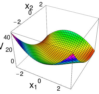
FIG. 1.: A three dimensional presentation of the potential energy surface for the landscape model for $\omega_{1}=1$, $\omega_{2}=2$, $\beta=-1$.

The potential energy has a local minimum at the origin where the energy is zero, and a pair of saddle points at $(x^{1},x^{2})=(\pm\sqrt{2}\omega_{1}\omega_{2}/(2\beta),-\omega_{1}^{2}/(2\beta))$, where the potential energy is $\omega_{1}^{4}\omega_{2}^{2}/(8\beta^{2})$. The model derives its name from the landscape-like potential energy surface. Note that, in contrast to a real landscape, the potential energy decreases without bound beyond the saddle points. Quantum mechanically, this allows a particle to escape from the potential well, for instance, by tunneling through in the neighborhood of the saddle point and moving to infinity as, e.g., in the case of nuclear fission. This analogy was one of the reasons for introducing the model.

We discuss this model with the help of the potential energy function, $V$, and the square of its gradient, $U$. The generalized valley equation,

$$V_{,\alpha}=\Omega U_{,\alpha},$$ (136)

can be reduced to a single equation by eliminating $\Omega$,

$$0 = V_{,1}U_{,2}-V_{,2}U_{,1}$$ (137)

$$= -x^{1}\left\{4(x^{2})^{3}\beta^{2}\omega_{2}^{2}+4(x^{2})^{2}\left[\beta\omega_{2}^{2}\omega_{1}^{2}-(x^{1})^{2}\beta^{3}\right]\right.$$ (139)

$$\left.\qquad+2x^{2}\left[(x^{1})^{2}\beta^{2}(\omega_{2}^{2}-2\omega_{1}^{2})-\omega_{2}^{4}\omega_{1}^{2}+\omega_{2}^{2}\omega_{1}^{4}\right]+2(x^{1})^{4}\beta^{3}-(x^{1})^{2}\beta\omega_{1}^{2}(\omega_{2}^{2}+\omega_{1}^{2})\right\}.$$

Here we have exhibited the generalized valley equation suggestively as a cubic equation for $x^{2}$, with coefficients that are functions of $x^{1}$. Of the three solutions of the cubic, one corresponds to a path that connects the minimum with the saddle point, following the direction of steepest descent near the saddle, and the other two describe a closed path that corresponds to the direction of steepest ascent near the saddle. Of course we restrict our attention to the first type of solution.

FIG. 2.: The solution of the valley equation (solid line) for $\omega_{1}=1$, $\omega_{2}=2$, $\beta=-1$. The thin solid and dashed lines are contours of the potential energy.

In Fig. 2 we show the solution of the valley equation, for the parameters $\omega_{1}=1$, $\omega_{2}=2$, $\beta=-1$, as the solid line, drawn on a background of the contours of the potential energy. As one can see, the valley passes through the minimum and the saddle points.

FIG. 3.: The solution of the valley equation (solid line) for $\omega_{1}=1$, $\omega_{2}=1.2$, $\beta=-1$. The thin solid and dashed lines are contours of the potential energy.

We also show the same solution for a different $\omega_{2}$, $\omega_{2}=1.2$, in Fig. 3 Although the solution looks similar, one should notice the larger curvature of the valley near the origin. We shall show that this indicates poorer decoupling.

Before considering the matter of decoupling, let us first discuss alternative methods to determine an approximately decoupled manifold. As described in Sec. II C, we can use the local harmonic equation, which takes a particularly simple form here because the metric tensor is the unit matrix,

$$V_{,\alpha}^{\beta}f^{\mu}_{,\beta}=\Omega^{2}_{\mu}f^{\mu}_{,\alpha}.$$ (140)

It is supplemented by the force condition

$$V_{,\alpha}=\lambda f^{1}_{,\alpha}.$$ (141)

Replacing $f^{1}$ by $V_{,\alpha}/\lambda$ in (140), we find

$$\Omega_{1}^{2}V_{,\alpha}=V_{,\alpha}^{\beta}V_{,\beta}=U_{,\alpha},$$ (142)

which shows that the local harmonic equation for the decoupling of one coordinate is equivalent to the valley equation, a result already known to us.

It is of some interest to consider an alternative to the subsidiary condition Eq. (141). Because of the simple metric, given a value of $f^{1}_{,\alpha}$, it and the associated value of $g^{\alpha}_{,1}$ are proportional to each other; thus the latter may replace the former in Eqs. (140) and (141) since covariant and contravariant derivatives are now identical. In the case of exact decoupling we would find that $V_{,\alpha}$ is parallel to the path $g^{\alpha}_{,1}$. In the present model this can not be true, since we do not have exact decoupling. Thus the condition that $g_{,1}^{\alpha}$ is parallel to the path is different from Eq. (141). We thus obtain a second algorithm by combining Eq. (140) for $g^{\alpha}_{,1}$ with the condition that the latter be along the path, namely

$$g_{,1}^{\alpha}=dx^{\alpha}/dq,$$ (143)

which serves as replacement for Eq. (141). For the model at hand, we know from the solution of the GVE that the collective path can be parameterized as

$$x^{1}=q,\;\;\;x^{2}=h(q),$$ (144)

which would give

$$g_{,1}^{\alpha}=(1,h^{\prime}(q)).$$ (145)

If we use this in the local harmonic equation, we find that

$$V_{,11}+V_{,12}h^{\prime} = \Omega^{2},$$ (146a)

$$V_{,21}+V_{,22}h^{\prime} = \Omega^{2}h^{\prime}.$$ (146b)

Using Eq. (146a) to eliminate $\Omega^{2}$ in the second equation, we find a quadratic equation for $h^{\prime}$ that can be converted to an ordinary differential equation by solving for $h^{\prime}$, (note that the derivatives of $V$ are functions of $q$ and $h(q)$)

$$h^{\prime}=\frac{(V_{,22}-V_{,11})\pm\sqrt{(V_{,22}-V_{,11})^{2}+4V_{,12}V_{,21}}}{2V_{,12}}.$$ (147)

This differential equation is solved as an initial value problem, integrating outward from the point $x^{1}=0,x^{2}=0$, i.e., $h(0)=0$. Since we would like to find that solution that is as close to the valley as possible, we choose the minus sign in Eq. (147), so that $h^{\prime}(0)=0$ as well.

The solutions to this modified local harmonic equation are shown in Figs. 2 and 3 by the dashed lines. They follow the valley closely, but not exactly. For that reason they do not pass through the saddle point. This shows that the GVA and the usual form of the LHA have some advantage over this form of the local harmonic equation.

Now that we have calculated the valley we can easily calculate the collective potential energy as

$$\bar{V}(q)=V(q,x^{2}(q)).$$ (148)

If we wish to calculate the collective mass we need to have a set of basis vectors. As discussed in Sec. II B 3, there are at least two natural choices that can be made, which lead to the same collective mass in the case of exact decoupling. In general, i.e., when decoupling is not exact, as just stated above, these two sets will not lead to the same answer. The first definition of the mass is based on the tangent vector,

$$g^{\alpha}_{,1}=dx^{\alpha}/dq=(1,dx^{2}/dx^{1}),$$ (149)

so that the inverse mass can be evaluated as

$$\bar{B}_{11}=g^{\alpha}_{,1}B_{\alpha\beta}g^{\beta}_{,1}=1+(dx^{2}/dx^{1})^{2}.$$ (150)

The other definition of the mass is based on the covariant form of the gradient of $V$,

$$V_{,\alpha} = \bar{V}_{,q}f^{1}_{,\alpha}$$ (151)

$$= (V_{,\alpha}g^{\alpha}_{,1})f^{1}_{,\alpha}$$ (152)

$$= (V_{,1}+V_{,2}dx^{2}/dx^{1})f^{1}_{,\alpha},$$ (153)

so that we find

$$\breve{B}^{11} = f^{1}_{,\alpha}B^{\alpha\beta}f^{1}_{,\beta}$$ (154)

$$= [(V_{,1})^{2}+(V_{,2})^{2}]/[V_{,1}+V_{,2}(dx^{2}/dx^{1})]^{2}.$$ (155)

We use the inverse of Eq. (150) as our definition of the collective mass, i.e.,

$$\bar{B}^{11}=1/[1+(dx^{2}/dx^{1})^{2}].$$ (156)

As stated before the difference between $\bar{B}$ and $\breve{B}$ is related to the quality of decoupling. For that reason we evaluate

$$D=|\bar{B}_{11}\breve{B}^{11}-1|.$$ (157)

Let us now look at the behavior of $\bar{V}$, $\bar{B}$ and $D$ for the two sets of parameters considered.

FIG. 4.: The solution to the collective path for the landscape model for $\omega_{1}=1$, $\omega_{2}=2$, $\beta=-1$. In panel (a) we show the collective potential energy, in panel (b) the collective mass, and panel (c) contains the decoupling parameter $D$.

We have plotted these three quantities for $\omega_{1}=1$, $\omega_{2}=2$, $\beta=-1$ in Fig. 4. As can be seen from the value of the decoupling measure $D$, Fig. 4c, decoupling is very good. In Fig. 4b we can see that the mass changes only very slowly along the path, another indication that the decoupling is excellent.

FIG. 5.: The solution to the collective path for the landscape model for $\omega_{1}=1$, $\omega_{2}=1.2$, $\beta=-1$. In panel (a) we show the collective potential energy, in panel (b) the collective mass, and panel (c) contains the decoupling parameter $D$.

If we once again reduce $\omega_{2}$ to $1.2$ (Figs. 5), we find much larger values for $D$ as illustrated in Fig. 5c. The collective mass $\bar{B}$ also shows a much more pronounced change. These are all indications of poorer decoupling.

2 Three-dimensional model

In order to illustrate the process of decoupling two coordinates (out of three) we use a model which is a simple generalization of the model of the previous section to one more dimension,

$$H=\mbox{$\frac{1}{2}$}[p_{1}^{2}+p_{2}^{2}+p_{3}^{2}]+\mbox{$\frac{1}{2}$}[\omega_{1}^{2}(x^{1})^{2}+\omega_{2}^{2}(x^{2})^{2}+\omega_{3}^{2}(x^{3})^{2}]+\beta[(x^{1})^{2}+(x^{2})^{2}]x^{3}.$$ (158)

The potential energy has one minimum, at ${{\mathbf{x}}}=0$, and two pairs of saddle points (at ${{\mathbf{x}}}=(\pm\omega_{1}\omega_{3}/[\beta\sqrt{2}],0,\omega_{1}^{2}/[2\beta])$ and ${\mathbf{x}}=(0,\pm\omega_{2}\omega_{3}/[\beta\sqrt{2}],\omega_{2}^{2}/[2\beta])$. These saddle points are connected through shallow one-dimensional valleys with the minimum at the origin.

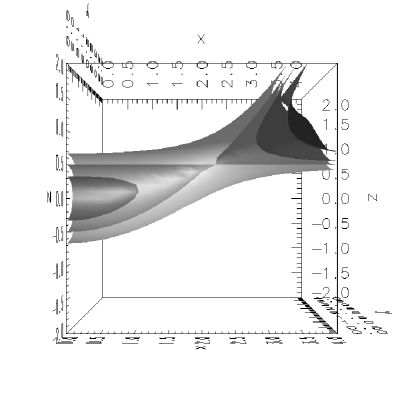
FIG. 6.: A set of isopotential surfaces for the 3D landscape model ($\omega_{1}=1$, $\omega_{2}=2$, $\omega_{3}=3$, $\beta=-1$). From dark to light the energy values are -1, 0.5, 9/8 and 2. We clearly see the saddle point for $x_{2}=0$ at $V=9/8$. For conciseness we have labeled the axes with $x$, $y$ and $z$, rather than $x_{1},x_{2},x_{3}$. The range on the $y$ axis ranges from 0 to 4.

This can clearly be seen in Fig. 6, where we show a set of isopotential surfaces for the potential energy. These show clearly the minimum at the origin, connected through a saddle point to the region of unbounded negative energy.

To decouple two coordinates out of three we need three scalar functions. In this study we use the potential $V$, $U=\sum_{i}(\partial V/\partial x^{i})^{2}/2$ and $W=\sum_{i}(\partial U/\partial x^{i})^{2}/2$. By elimination of the Lagrange multipliers the generalized valley equation can be converted into an equation for the vanishing of a determinant,

$$\left|\begin{array}[]{ccc}V_{,1}&U_{,1}&W_{,1}\\ V_{,2}&U_{,2}&W_{,2}\\ V_{,3}&U_{,3}&W_{,3}\end{array}\right|=0.$$ (159)

By explicit evaluation we can show that, for fixed $x^{1}$ and $x^{2}$, this equation is a sixth order polynomial equation for $x^{3}$, and as such the solutions may be very complex. Furthermore, the equation has the trivial solutions $x^{2}=0$ and $x^{1}=0$. In the following discussion we always discuss the determinant divided by the factor $x^{1}x^{2}$.

We have studied this equation for $\omega_{1}=1$, $\omega_{2}=2$, $\omega_{3}=3$ and $\beta=-1$. The potential energy is symmetric under the transformation $x^{1}\rightarrow-x^{1}$, as well as under $x^{2}\rightarrow-x^{2}$, so that we need only to consider the region $x^{1}\geq 0$, $x^{2}\geq 0$. Near the point $x^{1}=0$, $x^{2}=0$ we find that the GVE has only two real solutions, only one of which passes through ${\mathbf{x}}=0$. We now wish to study this last solution. In order to be able to present clearly what is happening, we have drawn graphical representations of one-dimensional slices of the solutions to the GVE, $x^{3}(x^{1},x^{2})$.

  

FIG. 7.: Three slices through the surface for the solution to the valley equations for $\omega_{1}=1$, $\omega_{2}=2$, $\omega_{3}=3$ and $\beta=-1$. In panel (a) we show the case $x^{2}=0$, in panel (b) $x^{1}=0$ and in panel (c) $x^{1}=x^{2}$.

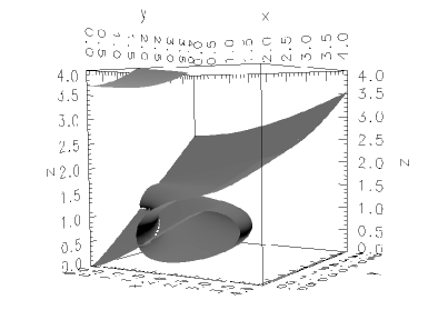
FIG. 8.: A three dimensional representation of the solution to the GVA sketched in Fig. 7

The two slices shown in Figs. 7a and  7b, for $x^{2}=0$ and $x^{1}=0$, contain both the minimum and a saddle point. In that case we encounter a result that is familiar from the case of decoupling in two dimensional models: a second solution crosses the valley at the saddle point. For the sake of clarity we have enlarged the region of the crossing in the inset in Figs. 7. The result is not too surprising once one realizes that we have a one-dimensional valley solution for both $x^{2}=0$ and $x^{1}=0$. The two cuts represented here are just these solutions.

The situation is very different, however, if we take any other cut through the $x^{1}$–$x^{2}$ plane. A representative case, for $x^{1}=x^{2}$ is presented in Fig. 7c. We find that on a course scale we do not see any difference in behavior, i.e., we see a crossing, but if we enlarge the region of the crossing we see that the crossing does not really take place. All the features illustated in Fig. 7 can be obtained from suitable cuts of the three-dimensional surface sketched in Fig. 8.

The avoided crossing appears not to be due to a numerical artifact. In an attempt to understand the situation we have just described, we have studied the alternative procedure for defining an approximately decoupled surface, based on the second form of the fundamental decoupling theorem developed in Sec. II B 1. This is the form that makes direct use of simplified vector fields rather than proceeding from point functions and is more directly tied to the local harmonic approximation when there is not exact decoupling. In this approach, we have already shown that $V_{,\alpha}$, $U_{,\alpha}=V_{,\alpha}^{~{}\beta}V_{,\beta}$, $\tilde{W}_{,\alpha}=V_{,\alpha}^{~{}\beta}V_{,\beta}^{~{}\gamma}V_{,\gamma}$ must be a set of three dependent vectors, since they are all three linear combinations of $f^{1}$ and $f^{2}$. From this linear dependence we once again obtain a determinant that should be zero,

$$\left|\begin{array}[]{ccc}V_{,1}&U_{,1}&\tilde{W}_{,1}\\ V_{,2}&U_{,2}&\tilde{W}_{,2}\\ V_{,3}&U_{,3}&\tilde{W}_{,3}\end{array}\right|=0.$$ (160)

This equation looks very similar to the GVE, but numerical study shows that it does not suffer from the avoided crossing problems noted for the GVA.

We shall now explain why the GVA and the LHA give different results. First consider the situation with respect to stationary paths in the model under study. These are of course solutions to the “valley” equation $V_{,\alpha}-\Omega_{1}U_{,\alpha}=0$. In addition to the two valleys that bound the part of the decoupled surface under study, there will be a ridge connecting the two associated saddle points. It is an easy consequence of the equations of the LHA that because along such an extremal path $V_{,\alpha}$ degenerates into proportionality to a definite solution of the local harmonic equation (rather than being a linear combination of such solutions, the general case), that not only are $V_{,\alpha}$ and $U_{,\alpha}$ parallel to each other as required by the valley equation but each is also parallel to $\tilde{W}_{,\alpha}$. Therefore along the ridge in question the modified GVA equation (160) does not determine a local tangent plane, but instead only a single direction common to the two intersecting surfaces, an intersection that takes place along the ridge. If, however, in the generalized valley equation we replace $\tilde{W}_{,\alpha}$ by another vector field belonging to the set named in the fundamental theorem, then as long as decoupling is not exact, this alternate third vector field will not in general be parallel to the first two, and a local tangent plane will be determined. If the different choices do not differ radically, however, we must expect the phenomenon encountered, namely a near crossing.

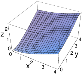
FIG. 9.: The solution to the LHA equations for $\omega_{1}=1$, $\omega_{2}=2$, $\omega_{3}=3$ and $\beta=-1$.

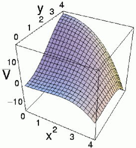
FIG. 10.: The collective potential energy for the LHA surface shown in Fig. 9.

It is simplest, therefore, to restrict our attention to the solution $x^{3}(x^{1},x^{2})$ obtained from the LHA. We have drawn that solution that runs through both saddle points and the minimum in Fig. 9. We also show the behavior of the collective potential energy in Fig. 10. One can distinguish the presence of two shallow valleys along the $x^{1}$ and $x^{2}$ axis. That the surface $x^{3}(x^{1},x^{2})$ obtained from the local harmonic equation is very close to a solution of the GVA, except in the region of the crossing can be seen in Fig. 11. In that figure we plot $\Delta$, the difference between the solution of the LHA for fixed $x_{1},x_{2}$ and the nearest real solution to the GVA. The difference is small, but grows as $x^{1}$ and $x^{2}$ both increase.

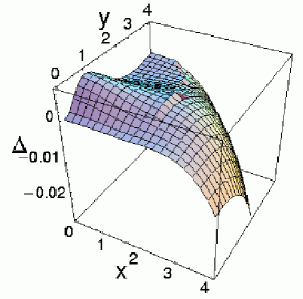
FIG. 11.: The difference between the LHA surface shown in Fig. 9 and the nearest solution to the GVA.

FIG. 12.: The decoupling measure $D$ for the LHA surface shown in Fig. 9.

It now remains to discuss the quality of decoupling. With our definition of the collective surface as $x^{3}(x^{1},x^{2})$ we easily obtain

$$g^{\alpha}_{,1} = (1,0,\partial x^{3}/\partial x^{1}),$$ (161a)

$$g^{\alpha}_{,2} = (0,1,\partial x^{3}/\partial x^{2}).$$ (161b)

The inverse collective mass now can be calculated as

$$\bar{B}_{ij}=\sum_{\alpha}g^{\alpha}_{i}g^{\alpha}_{j}.$$ (162)

We can also derive a set of vectors from the gradients of $V$ and $U$,

$$V_{,\alpha} = \bar{V}_{,1}f^{1}_{,\alpha}+\bar{V}_{,2}f^{2}_{,\alpha},$$ (163)

$$U_{,\alpha} = \bar{U}_{,1}f^{1}_{,\alpha}+\bar{U}_{,2}f^{2}_{,\alpha}.$$ (164)

[Here we use the chain rule, $\bar{X}_{,i}=X_{,\alpha}g^{\alpha}_{,i}$]. This can be inverted to give $f^{1}$ and $f^{2}$, with suitable limits taken if the determinant $\left|\begin{array}[]{cc}\bar{V}_{,1}&\bar{U}_{,1}\\ \bar{V}_{,2}&\bar{U}_{,2}\end{array}\right|$ equals zero. We thus obtain

$$\breve{B}^{ij}=\sum_{\alpha}f_{,\alpha}^{i}f_{,\alpha}^{j}.$$ (165)

We can now define the decoupling measure $D$:

$$D=\left|\Bigl{[}\mbox{$\frac{1}{2}$}\sum_{ij}\bar{B}_{ij}\breve{B}^{ji}\Bigr{]}-1\right|.$$ (166)

This quantity is displayed in Fig. 9. As can be seen it is relatively small, showing its largest values for $x^{1}=0$. This is where the second and third eigenvalues of the local harmonic equation are closer than for other points in the $x^{1}$–$x^{2}$ plane, so that the decoupling is poorer. Nevertheless, the results we have found show excellent overall decoupling.

Apart from the problem with avoided crossings that we have discussed in detail, there do not appear to be major differences between the results obtained from the generalized valley equations and from the local harmonic approximation. The fact that there are these avoided crossings may lead to a slight prejudice in favor of the LHA, even though we would like to point out that from a physical point of view, in contrast to the mathematical discussion given above, we can easily “span the gap” by interpolation, making it less problematic to work with the GVA.

B A simplified model for tunneling in many-particle systems

1 Description of the model

As a more substantial example of the methods developed in the previous sections, we consider a model of a system of $N$ oscillators, each assigned as well a half unit of spin. The Hamiltonian is chosen to be of such a simple form that the model is equivalent to an oscillator in interaction with a spin system that is almost classical. This model was studied first in [49] by quite different methods. The following discussion is based on Ref. [20].

The system to be studied is described by the Hamiltonian,

$$H=\sum_{i=1}^{N}\frac{1}{2}\left(p^{2}_{i}+q^{2}_{i}\right)+\kappa\left(\sum_{i=1}^{N}q_{i}\right)\left(\sum_{i=1}^{N}\sigma_{zi}\right)-\lambda\left(\sum_{i=1}^{N}\sigma_{xi}\right)^{2}.$$ (167)

One sees that only the center of mass is coupled to the total spin and the internal motion is unaffected by interaction. This leads to a tremendous simplification, if we introduce the new variables

$$q = \frac{1}{\sqrt{N}}\sum_{i=1}^{N}q_{i},\;\;p=\frac{1}{\sqrt{N}}\sum_{i=1}^{N}p_{i},$$ (168)

$$S_{k} = \frac{1}{2}\sum_{i=1}^{N}\sigma_{ki},\;k=x,y,z,$$ (169)

as well as $N-1$ relative variables. The Hamiltonian (167) then separates into an uninteresting piece, representing the uncoupled relative oscillators, and the interesting part,

$$H^{\prime}=\frac{1}{2}p^{2}+\frac{1}{2}q^{2}+2\kappa\sqrt{N}qS_{z}-4\lambda S^{2}_{x}.$$ (170)

Henceforth we replace $H^{\prime}$ by $H$. We shall also set $N=2J$ throughout this discussion, where $J$ is the value of the “angular momentum” for the band of states which can be shown to include the ground state.

2 Study of the classical limit by the generalized valley algorithm

In order to study the Hamiltonian (170) by the methods of Secs. II B and II C, it is convenient to introduce a mapping of the $su(2)$ algebra onto a pair of quantum action-angle variables $\Pi$ and $\xi$ according to the formulas [50, 51] (the non-standard choice of the quantization axis is related to the form of the Hamiltonian)

$$S_{+} = (S_{-})^{\dagger}=S_{z}+iS_{x}$$ (171)

$$= \exp\left(\mbox{$\frac{1}{2}$}i\xi\right)\sqrt{(J+(1/2))^{2}-\Pi^{2}}\exp\left(\mbox{$\frac{1}{2}$}i\xi\right)$$ (172)

$$= \exp(i\xi)\sqrt{J(J+1)-\Pi(\Pi+1)},$$ (173)

$$S_{y} = \Pi,$$ (174)

where

$$[\Pi,\exp(i\xi)]=\exp(i\xi).$$ (175)

From these equations, we obtain approximate formulas for $S_{z}$ and $S_{x}^{2}$, required for the evaluation of Eq. (170), by expanding in powers of $(\Pi/J)$, assuming $\Pi$ to be no larger than of order unity. (This assumption will have to be confirmed a posteriori to be valid for the states of interest to us.) These formulas are

$$S_{z} = \sqrt{J(J+1)}\cos(\xi)-\frac{1}{4\sqrt{J(J+1)}}\{\cos(\xi),\Pi^{2}\},$$ (176a)

$$S_{x} = \sqrt{J(J+1)}\sin(\xi)-\frac{1}{4\sqrt{J(J+1)}}\{\sin(\xi),\Pi^{2}\},$$ (176b)

$$S_{x}^{2} = J(J+1)\sin^{2}(\xi)-\frac{1}{4}\{\sin(\xi),\{\sin(\xi),\Pi^{2}\}\},$$ (176c)

where the braces stand for the anticommutator of the corresponding operators. The Hamiltonian (170) thus becomes

$$H = V(q,\xi)+T,$$ (177a)

$$V(q,\xi) = \frac{1}{2}q^{2}+2\kappa q\sqrt{2J^{2}(J+1)}\cos(\xi)-4\lambda J(J+1)\sin^{2}(\xi),$$ (177b)

$$T = \frac{1}{2}p^{2}-\kappa q\frac{1}{\sqrt{2(J+1)}}\{\cos(\xi),\Pi^{2}\}+\lambda\{\sin(\xi),\{\sin(\xi),\Pi^{2}\}\}.$$ (177c)

The above expression for $H$ contains correctly the classical limit plus the corrections of order $1/J$. The choice of variables made in Eqs. (173) and (174) has the great advantage that most of the burden of variation of the spin variables is carried by the trigonometric functions of $\xi$ and that $\Pi$ remains small in the domain of interest to us.

Passing to the classical limit, we may rewrite the kinetic energy as

$$T_{{\rm class}}=\frac{1}{2}p^{2}+\frac{1}{2}B_{\xi}(q,\xi)\Pi^{2},$$ (178)

where

$$B_{\xi}(q,\xi)=8\lambda\sin^{2}(\xi)-\kappa q\frac{4}{\sqrt{2(J+1)}}\cos(\xi),$$ (179)

and we find that the inverse mass matrix is diagonal

$$B=\left(\begin{array}[]{cc}1&0\\ 0&B_{\xi}\end{array}\right).$$ (180)

FIG. 13.: The profile of the potential energy surface $V(q,\xi)$.

In the remainder of this section we shall use the choice of parameters $\kappa=0.006403$, $\lambda=0.0005$ and $N=40$, the same as used in [49]. The profile of the potential energy function, $V(q,\xi)$, for this choice of parameters is displayed in Fig. 13, where one can easily see a valley, the precise course of which is defined below by the solution of Eqs. (183) and (184). We take $\xi$ in the range $0\leq\xi\leq 2\pi$. One computes that $V$ is minimum at $\xi=n\pi$ and $q=-2\kappa\sqrt{2J^{2}(J+1)}\cos(\xi)$, with

$$V_{{\rm min}}=-4\kappa^{2}J^{2}(J+1),$$ (181a)

and $$V q=0,\xi=(2n+1)\pi/2$$ has saddle points at , with

$$V_{{\rm saddle}}=-4\lambda J(J+1).$$ (181b)

We thus identify a potential barrier of height

$$V_{{\rm barrier}}=4J(J+1)(J\kappa^{2}-\lambda).$$ (181c)

We now turn to the machinery of our method. To apply the valley algorithm, one constructs the point function

$$U(q,\xi)=\frac{1}{2}(V_{,q}^{2}+B_{\xi}(q,\xi)V_{,\xi}^{2})$$ (182)

and solves the equations

$$V_{,q}-\omega U_{,q} = 0,$$ (183)

$$V_{,\xi}-\omega U_{,\xi} = 0,$$ (184)

where by subscripts we denote the corresponding partial derivatives and $\omega$ is a Lagrange multiplier. These are the equations of a valley on the potential energy surface as seen from the standpoint of a metric defined by the classical kinetic energy (179).

For the case of two coordinates one can simplify these equations to a single algebraic equation, the determinantal condition

$$\left|\begin{array}[]{ll}V_{,q}&U_{,q}\\ V_{,\xi}&U_{,\xi}\end{array}\right|=0.$$ (185)

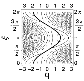
FIG. 14.: The collective path obtained as a solution of Eqs. (183) and (184).

FIG. 15.: The collective potential energy, $V_{\text{coll}}=V(g(x),x)$.

We shall parameterize the collective path by choosing a collective coordinate $x$ defined by the equations

$$\xi=x,\;\;\;q=g(x).$$ (186)

The collective path and collective potential energy that result from solving Eqs. (183) and (184) are displayed in Figs. 14 and 15, respectively. The latter is given by the formula where we use the notation that a bar denotes a function of collective variables only,

$$\bar{V}(x)=V(q(x),\xi(x)).$$ (187)

Turning to the consideration of the collective mass, the theory provides two distinct formulas, which agree only when there is exact decoupling. This can be understood physically as follows: The collective path (186) is the locus of points for which $\nabla V$ and $\nabla U$ are parallel, as seen from Eqs. (183) and (184). Exact decoupling occurs when the joint direction of these vectors coincides with the tangent to the collective path. The formula for the mass that is determined by the tangent vector to the collective path, which is an application of Eq. (150), is

$$\bar{B}^{-1}=\frac{1}{B_{\xi}}\left(\frac{d\xi}{dx}\right)^{2}+\left(\frac{dq}{dx}\right)^{2}=\frac{1+B_{\xi}g_{,x}^{2}}{B_{\xi}},$$ (188)

where

$$\left(\begin{array}[]{cc}1&0\\ 0&{1}/{B_{\xi}}\end{array}\right),$$ (189)

is the inverse of the metric tensor, Eq. (180). The quantity $\bar{B}$ is plotted in Fig. 16.

FIG. 16.: The inverse collective mass, $\bar{B}=B_{\xi}(1+g_{x}^{2}B_{\xi})^{-1}$.

If, however, the decoupling is not exact, we can derive an alternative formula for the mass by replacing the components of the tangent vector in Eq. (188) by the components of a corresponding vector parallel to ${\mathbf{\nabla}}V$. This gives the formula

$$\breve{B}=\frac{V_{,q}^{2}+BV_{,\xi}^{2}}{(V_{,q}g_{,x}+V_{,\xi})^{2}}.$$ (190)

In Sec. II B 3 we have suggested an invariant measure, $D$, of the goodness of decoupling, which is a point function on the collective surface. For the case of a collective path, it reduces to the intuitive measure

$$D=|(\breve{B}-\bar{B})\bar{B}^{-1}|.$$ (191)

This quantity is plotted in Fig. 17. As one can see from this plot, the collective mass computed using two independent methods is practically the same, the differences being not larger than 0.012 percent. This simply means that in this case the collective branch of the spectrum is almost completely decoupled from the non-collective one. This result will be reflected when we assess the accuracy of our quantum results.

FIG. 17.: The invariant measure of the decoupling, Eq. (191).

The theory discussed thus far does not pertain at all to the stability of the motion in the neighborhood of the collective path. This is determined by the frequency for vibration along the local direction perpendicular to the collective path, as given by a formula which can be deduced from the considerations of Sec. II B 4,

$$\omega^{2}_{\rm NC}=\frac{V_{,\xi\xi}(B_{\xi}g_{,x})^{2}-2V_{,\xi q}B_{\xi}g_{,x}+V_{,qq}}{1+B_{\xi}g_{,x}^{2}}.$$ (192)

As seen from the plot in Fig. 18, the required stability is established. This completes our discussion of the classical part of the problem.

FIG. 18.: The square of the frequency of non-collective vibrations, Eq. (192).

 

We provide a brief derivation of formula (192). We use index $1$ for the collective mode, $2$ for the non-collective mode. Given the basis vector $g^{\alpha}_{,1}=(1,g_{,x})$ following from Eq. (186), we calculate $g^{\alpha}_{,2}$ by the procedure described at the end of Sec. II B 4. This yields the basis vector

$$g^{\xi}_{,2} = -\frac{g_{x}B_{\xi}}{\sqrt{1+B_{\xi}g_{x}^{2}}},$$ (193)

$$g^{q}_{,2} = \frac{1}{\sqrt{1+B_{\xi}g_{x}^{2}}},$$ (194)

$$\bar{B}_{22} = 1.$$ (195)

Because of the choice (195), the square of the non collective frequency has the value $\bar{V}_{22}$, whose value, in the light of Eqs. (193) and (194) is given by Eq. (192).

 

3 Requantization and comparison with exact diagonalization

The next step is the quantization of the collective Hamiltonian in order to find the collective states. Given the collective mass ${\bar{B}}^{-1}$ and the collective potential energy ${\bar{V}(\xi)}$, we choose the corresponding quantized Hamiltonian in the form

$$H=\frac{1}{8}\{\Pi,\{\Pi,{\bar{B}}\}\}+{\bar{V}}(\xi),$$ (196)

where the commutation relation between $\xi$ and $\Pi$ is to be taken in the form (175), and $0\leq\xi\leq 2\pi$ with periodic boundary conditions. There are always some ambiguities in the quantization procedure, that arise from different orderings of the coordinate and momentum operators, but for a well defined collective motion they all differ by terms of relative order $1/J^{2}$ in the potential energy. For the choice made above, the corresponding classical Hamiltonian, obtained after a Wigner transformation, is exactly that found in the previous section. The quantum results that follow for the “ground-state-band” are reported in Table I. In the first two columns we list the exact and approximate (LACM) mean excitation energies of the doublets. The resulting decimal logarithms of the energy splittings for the first five levels are given in columns 3-5. The exact values listed in Table I were provided by the authors of [49]. The approximate method used by them, imaginary time-dependent Hartree-Fock (ITDHF), could be applied only to the doublet splittings, and can not be used to determine the individual eigenfunctions. Our values, on the other hand, were obtained as actual differences of eigenvalues.

TABLE I.: The mean excitation energies and the decimal logarithms of the splittings of the energy levels below the barrier. Column 1 displays exact values for the mean energies of the doublets, column 2 our results (LACM) for these values. Columns 3-5 contain exact, ITDHF, and LACM values for the doublet splittings.

Energy (Ref. [49])	Energy(LACM)	Exact (Ref. [49])	ITDHF (Ref. [49])	LACM
G.S.	G.S.	13.00	13.00	12.89
0.154	0.154	8.96	8.57	8.89
0.289	0.288	5.92	5.39	5.87
0.403	0.401	3.51	2.85	3.51
0.489	0.487	1.92	1.00	1.92

For all the levels below the barrier, the agreement with the exact results are very good. The fact that both the mean excitation energies and the splittings are well reproduced means that the formalism presented is accurate for the description of both the classically allowed and forbidden regions. The values of the mean excitation energies are defined by the collective mass and potential energy in the classically allowed region, while the splittings depend on the properties of the collective Hamiltonian in the classically forbidden region.

C A model of molecular isomerization

1 Introduction

The next application, which also involves a tunneling process, was stimulated by connection with an important molecular phenomenon known as isomerization. This refers to a situation where the ground state is (essentially) degenerate with respect to the transfer of one Hydrogen bond to an equivalent position by tunneling. We shall study a simplified model for the influence of the vibrational degrees of freedom on the tunneling rate. We shall concentrate first on the application of the GVA to a class of model Hamiltonians which couple a double well to an oscillator degree of freedom. We refer to our paper [26] for a discussion of the relationship of this effort to work done in the chemistry community on similar models. Aside from the specific problem of isomerization, there is an important class of applications associated with the concept of reaction path, based on the assumption that a chemical reaction proceeds along a valley path of the potential energy of the composite system, connecting neighboring minima through a saddle point. For the models treated specifically, the equations specifying the valley reduce to the problem of finding the zeros at each point of the collective path of a relatively simple determinant, the same result as encountered in the previous applications in this section. This method is not applicable to realistic reaction path problems. In Ref. [26] we have suggested an algorithm suitable for this case that combines elements of both the GVA and the local harmonic approximation and bears some relation to the methods we shall develop for the nuclear structure problem.

Before turning to a detailed study of the models, we take note of an inherent simplification associated with molecular problems. Though our theory has been designed to deal with a general classical Hamiltonian of the form

$$H(\pi,\xi)=\mbox{$\frac{1}{2}$}\pi_{\alpha}B^{\alpha\beta}(\xi)\pi_{\beta}+V(\xi),$$ (197)

where $\xi$ and $\pi$ are an $N$-dimensional set of canonical coordinates and momenta, respectively, for the special case under study, the molecular Born-Oppenheimer problem, the mass-tensor $B$ is diagonal, and can even be made equal to the identity matrix by going to so-called mass-scaled coordinates. The most general form the inverse mass $B^{\alpha\beta}$ can take, without this last rescaling is thus

$$B=\left(\begin{array}[]{cccccc}m_{1}^{-1}&0&0&0&\ldots&0\\ 0&m_{1}^{-1}&0&0&\ldots&0\\ 0&0&m_{1}^{-1}&0&\ldots&0\\ 0&0&0&m_{2}^{-1}&\ldots&0\\ \vdots&\vdots&\vdots&\vdots&\ddots&\vdots\\ 0&0&0&0&\ldots&m_{N}^{-1}\end{array}\right).$$ (198)

In this case the tensor notation may seem somewhat superfluous, but it becomes more natural as soon as we go to other coordinate systems.

It is necessary to add a remark concerning quantization of the models to be studied. As discussed in Sec. II B 4, for motion near a decoupled surface, the classical Hamiltonian takes the form

$$H=\mbox{$\frac{1}{2}$}\bar{B}^{ij}p_{i}p_{j}+\bar{V}+\mbox{$\frac{1}{2}$}\left(\bar{B}^{ab}p_{a}p_{b}+\bar{V}_{,ab}q^{a}q^{b}\right),$$ (199)

where the motion orthogonal to the collective surface is harmonic. For stability of the generalized valley equation we must require that all frequencies be real, so that it will cost energy to move away from the collective surface. If the decoupling is not exact, we must add to the Hamiltonian (199) terms linear in $q^{a}$ and $p_{a}$. Still we shall assume that Eq. (199) remains a good approximation to the problem at hand, since the linear term should in general be small. We check stability of the approximate Hamiltonian by calculating the harmonic frequencies.

Of even greater weight in what follows is that the same local frequencies can also be used to calculate corrections to the collective potential energy when we requantize the problem. If we assume that the motion in the non-collective coordinates is much faster than the motion in the collective coordinates, the non-collective coordinates contribute only the zero-point energy of the (local) frequencies. One thus writes,

$$H=\frac{1}{8}\{\{p_{i},\bar{B}^{ij}\},p_{j}\}+\bar{V}+\sum_{a=K+1}^{N}(\mbox{$\frac{1}{2}$}\hbar\omega_{a})$$ (200)

for the quantum Hamiltonian. Here $\hbar\omega_{a}$ denote the local harmonic energies that depend on the collective coordinates $q^{i}$. Therefore the last term of Eq. (200) contributes to the collective potential energy. Calculating these frequencies is a standard small oscillations problem.

2 Definition of and application to a class of model problems

We now apply the GVA to a specific model, to show both the power and the drawbacks of our solution method. The model in question describes a two-dimensional tunneling phenomenon in a double-well potential, which can be thought of as a model of isomerization. The quantum Hamiltonian to be studied belongs to a class having the general form

$$H=\mbox{$\frac{1}{2}$}b_{0}\left(\frac{\partial^{2}}{\partial s^{2}}+\frac{\partial^{2}}{\partial Q^{2}}\right)+V(s,Q),$$ (201)

with

$$V(s,Q)=V_{0}(s)-f(s)Q+\mbox{$\frac{1}{2}$}m\omega^{2}Q^{2}.$$ (202)

Here $s$ denotes a first guess for the “reaction” coordinate and $Q$ is the coordinate of an orthogonal harmonic vibration. Because the mass matrix is constant, the point function $U$ becomes (to an overall scale)

$$U(s,Q)=\mbox{$\frac{1}{2}$}\left(V_{,s}^{2}+V_{,Q}^{2}\right).$$ (203)

The generalized valley equation states that the gradients of $V$ and $U$ are parallel, which in this case leads to the determinantal condition

$$V_{,s}U_{,Q}-V_{,Q}U_{,s}=0.$$ (204)

We parameterize the path by a variable $t$,

$$s=t,\;\;Q=q(t)$$ (205)

For the covariant collective mass, we thereby calculate, with dot indicating derivative with respect to $t$,

$$\bar{B}_{11}=(1+\dot{q}^{2})b_{0}^{-1},$$ (206)

whose reciprocal is $\bar{B}^{11}$. If we designate the basis vector defined by differentiating (205) as $g_{,1}=(1,\dot{q})$, then to study oscillations in the non-collective coordinate, we need an orthogonal basis vector $g_{,2}$, which can be chosen as

$$g_{,2}=(\dot{q},-1).$$ (207)

Thus we find

$$\bar{B}^{22}=\frac{b_{0}}{1+\dot{q}^{2}},$$ (208)

and, from Eq. (81)

$$\bar{V}_{,22} = g_{,2}\left(\begin{array}[]{cc}V_{,ss}&V_{,sQ}\\ V_{,Qs}&V_{,QQ}\end{array}\right)g_{,2}$$ (211)

$$= (V_{,ss}\dot{q}^{2}-2V_{,sQ}\dot{q}+V_{,QQ}).$$ (212)

For the harmonic frequency, associated at each point with the motion orthogonal to the path, we then find

$$\hbar\omega_{2}(t)=\sqrt{\frac{b_{0}}{1+\dot{q}^{2}}}\left.\sqrt{V_{,ss}\dot{q}^{2}-2V_{,sQ}\dot{q}+V_{,QQ}}\right|_{s=t,Q=q(t)}.$$ (213)

Except for the decoupling measure $D$, we have now gathered all the information needed to carry out a study of the models defined by (201) and (202). In order to calculate $D$ we need the basis vector $f^{1}$, designated as the breve basis vector in Secs. II B 2 and II B 3. We use the conditions

$$(V_{,s},V_{,Q})=\bar{V}_{,t}(f^{1}_{,s},f^{1}_{,Q})$$ (214)

to evaluate $f^{1}$ as

$$(f^{1}_{,s},f^{1}_{,Q})=(V_{,s}+\dot{q}V_{,Q})^{-1}(V_{,s},V_{,Q}).$$ (215)

Thus we find

$$\breve{B}^{11}=b_{0}(V_{,s}^{2}+V_{,Q}^{2})(V_{,s}+\dot{q}V_{,Q})^{-2},$$ (216)

from which, in combination with (206), we can easily evaluate $D$.

Turning to the models, since according to Eq. (202), the potential is a simple polynomial function of $Q$, we can readily derive, from Eq. (204), algebraic equations for $Q$ as a function of $s=t$. In general these are cubic equations, reducing to a quadratic equation if $f(s)$ is linear in $s$.

3 Harmonic and Gaussian potential

We have actually treated several distinct models [26] for the potential $V_{0}(s)$, but shall report on the one that has the most satisfactory physical properties. It is patterned after a choice [52] that has been made for the inversion potential of NH₃, and consists of the combination of a harmonic and a Gaussian potential:

$$H=-\mbox{$\frac{1}{2}$}\frac{\hbar^{2}}{m}\left(\frac{\partial^{2}}{\partial s^{2}}+\frac{\partial^{2}}{\partial Q^{2}}\right)+\mbox{$\frac{1}{2}$}[As^{2}+B(\mbox{e}^{-Cs^{2}}-1)]+\mbox{$\frac{1}{2}$}m\omega^{2}(Q-cs/m\omega^{2})^{2}.$$ (217)

Two of the three constants $A,B,C$ in the Hamiltonian were fixed by choosing the position of the minimum of the potential and the barrier height. The third constant was determined by a requirement that the maximal local frequency be relatively small (${\rm max}\,(d^{2}V(s,0)/ds^{2})\leq\,100\,{\rm kcal/(mol\AA^{2})}$). We thus made the choice

$$A = 27.87\;{\rm kcal/(mol\AA^{2})},$$ (218)

$$B = 23.27\;{\rm kcal/mol},$$ (219)

$$C = 7.17\;{\rm\AA^{-2}}.$$ (220)

FIG. 19.: Values for the tunneling splitting for the Hamiltonian (217). The frequency is $\omega=2980\;{\rm cm}^{-1}$. The continuous curve represents an exact result. The dashed curve is a calculation using the GVE approach, without zero-point corrections; the dotted curve is the result including quantum corrections.

FIG. 20.: Values for the tunneling splitting for the Hamiltonian (217). The frequency is $\omega=1333\;{\rm cm}^{-1}$. The continuous curve again represents an exact result. The dashed curve is a calculation using the GVA approach, without zero-point corrections; the dotted curve includes zero-point corrections.

FIG. 21.: Energy surface for Eq. (217), $c=1.05\;{\rm mdyn/\AA}$ and $\omega=2980\;{\rm cm}^{-1}$. The solution to the GVA is represented by the continuous curve. Note that it is almost a straight line!

We performed two sets of calculations, one for $m\omega^{2}=750\;{\rm kcal/(mol\AA^{2})}$ ($\omega=2980\;{\rm cm}^{-1}$) and another for $m\omega^{2}=150\;{\rm kcal/(mol\AA^{2})}$ ($\omega=1333\,{\rm cm}^{-1}$). We expect that adiabatic decoupling will be more accurate for the larger of the two frequencies, and this will be verified by our results. In Fig. 19 we show the results for the tunneling splitting for the larger value of $\omega$ as a function of $c$. The “exact” results were obtained by discretizing the Hamiltonian (217) on a grid. As can be seen we find perfect agreement with exact results up to fairly large $c$. There the splitting becomes extremely small, and we can not trust our exact results at that point. In Fig. 20 we show similar results for the smaller of the two frequencies. Our results are not as convincing as before, mainly due to the fact that the coupling is much stronger. This can also be seen from the paths followed: The path for $c=0.35\;{\rm mdyn/\AA}$ is practically a straight line for the largest of the two frequencies (Fig. 21), and has extremely good decoupling (Fig. 22), but in the second case has large curvature (Fig. 23) and poor quality of decoupling (Fig. 24).

In both Figs. 22 and 24 we have plotted not only the goodness of decoupling parameter $D$ but also another measure $E$,

$$E=\bar{V}_{,a}\bar{B}^{ab}\bar{V}_{,b}/U,$$ (221)

which is the ratio of the square of the magnitude of the force orthogonal to the collective surface to the square of the magnitude of the total force. Clearly there is a great similarity between the two measures.

FIG. 22.: The decoupling parameters $D$ and $E$ (Eq. (221)) for the path given in Fig. 21. The difference between $D$ and $E$ can not be seen on the scale of the picture. The overall size of the parameters is also quite small, indicating excellent decoupling.

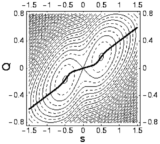
FIG. 23.: Energy surface for Eq. (217), $c=1.05\;{\rm mdyn/\AA}$ and $\omega=596\;{\rm cm}^{-1}$. The solution to the GVA is again represented by the continuous curve. Note that the oscillations are more pronounced than in Fig. 21.

FIG. 24.: The decoupling parameters $D$ (dashed) and $E$ (continuous) (Eq. (221)) for the path given in Fig. 22. The difference between $D$ and $E$ can only be seen near the maxima. The size of $D$ and $E$ indicates relatively poor decoupling.

4 Concluding remarks about simple applications

In this section we have discussed how to apply the GVA and LHA to simple models. By solving the relevant equations we find a path (or, in general, a surface) where we have optimal decoupling, in the sense that we retain some residual coupling both in the kinetic and potential energies.

Two of the examples chosen have involved decoupling one degree of freedom from a Hamiltonian containing two degrees of freedom. For another fully-worked example of the same general type, the so-called three-level Lipkin model, see [15]. We have also studied a case of decoupling two degrees of freedom from a system with three degrees of freedom [19, 28], choosing a generalization of the so-called landscape model [48]. The classical aspects of this model have been studied fully, but a quantization has not been carried out, since the potential energy is not bounded from below. For this model we placed special emphasis on the comparison between the GVA and LHA approaches. The local harmonic method may well be the one of choice for the many-body problem. Finally, we may view the methods developed and applied thus far as relevant to the problem of quantization of non-separable systems.

IV Applications to nuclear physics

From the applications to date, it is apparent that the methods developed are suitable for the decoupling of one and two degrees of freedom from a parent system with a few more degrees of freedom. Thus, as already remarked, they provide a useful approach to the approximate quantization of non-separable systems. The problem of major interest, however, is that of decoupling one or a few degrees of freedom from a system with many degrees of freedom, in particular, within the framework of the nuclear many-body problem. We were led to study this problem within a classical Hamiltonian framework from the well-known result [53, 54, 55, 56, 57] that the TDHF equations are equivalent to Hamilton’s equations. In this section we shall discuss the application of our ideas to realistic nuclear applications. This report is mainly based on our published work as referenced in the relevant sections. For some of our older applications we have redone calculations in a manner that is better suited to our current understanding of the correct approach. First we discuss how to transcribe the results of our previous work into the language of nuclear physics and begin the task of formulating and applying methods for solving the new equations. In the GVA version the latter will be seen to assume the form of a sequence of cranking equations, of which the first alone defines the conventional cranking theory [6]. The additional equations fully constrain the cranking operator, rather than leave its choice partly a matter of whim, as in existing theories. Indeed, the unambiguous determination of this operator is tantamount to fixing the approximately decoupled submanifold. An approximate method for solving the generalized cranking formulation is then described that reduces the many body problem to a few body problem of the type treated in our previous work. The application of this method is illustrated for several simplified models in Sec. IV C. In Sec. IV D we describe our study of the Silicon nucleus, and in Sec. IV E we recount our efforts to develop methods applicable to heavy nuclei.

A Transcription of the time-dependent hartree-fock theory to classical physics

1 Canonical variables and the adiabatic Hamiltonian

The material presented in this section is largely based on Ref. [25]. To utilize the theory described in the previous sections we must recast the TDHF(B) equations into the form of Hamilton’s equations. We shall utilize a method of our own devising. (In Appendix A, we describe various choices that have been suggested for carrying out this transformation.) As the simplest example we consider the TDHF equations,

$$i\dot{\rho}_{ab}=[{\cal H},\rho]_{ab},$$ (222)

where

$${\cal H}_{ab}=h_{ab}+V_{acbd}\rho_{dc},$$ (223)

and $h_{ab}=h_{ba}^{\ast}$, $V_{abcd}=-V_{bacd}=-V_{abdc}=V_{cdab}^{\ast}$ are the matrix elements of the single-particle ($h$) and two-body ($V$) parts of a non-relativistic nuclear many-body Hamiltonian. The labels $a,b,\ldots$ refer to a complete orthonormal set of single particle functions $\phi_{a}$; this set will be further subdivided into a set $h$ occupied in the reference Slater determinant and an unoccupied set $p$. We have

$$\rho=\sum_{h}\phi_{h}^{\ast}\phi_{h},\;\;\;(\rho^{2})_{ab}=\rho_{ab}.$$ (224)

The most convenient choice of basis for exhibiting the canonical structure of (222) is a dynamical basis in which $\rho$ is instantaneously diagonal, i.e., where $\rho$ in (222) is diagonal. In this basis (222) is equivalent to the pair of equations

$$i\dot{\rho}_{ph} = {\cal H}_{ph}=\delta W_{\mathrm{HF}}/\delta\rho_{hp},$$ (225)

$$i\dot{\rho}_{hp} = -{\cal H}_{hp}=-(\delta W_{\mathrm{HF}}/\delta\rho_{ph}),$$ (226)

where

$$W_{\mathrm{HF}}[\rho]=h_{ab}\rho_{ba}+\frac{1}{2}V_{abcd}\rho_{ca}\rho_{db},$$ (227)

the Hartree Fock functional, serves as Hamiltonian. Equations (226) are already in Hamiltonian form, and we identify $\rho_{ph}$ and $\rho_{hp}=\rho_{ph}^{\ast}$ as a conjugate pair of complex canonical variables. We may also introduce real canonical coordinates $\xi$ and $\pi$,

$$\rho_{ph} = \frac{1}{\sqrt{2}}(\xi^{ph}+i\pi_{ph}),$$ (228)

$$\rho_{hp} = \frac{1}{\sqrt{2}}(\xi^{ph}-i\pi_{ph})=\frac{1}{\sqrt{2}}(\xi^{hp}+i\pi_{hp}).$$ (229)

In order to utilize the theory of point transformations developed in such detail in Sec. II, we can construct an adiabatic classical Hamiltonian by expanding $W_{\mathrm{HF}}$ in powers of $\pi$. With the help of (229), we find the standard Hamiltonian form,

$$H(\xi,\pi) \simeq W[\rho(\xi,0)]+\frac{1}{2}\pi_{ph}\pi_{p^{\prime}h^{\prime}}(\delta^{2}W/\delta\pi_{ph}\delta\pi_{p^{\prime}h^{\prime}})$$ (230)

$$\equiv V(\xi)+\frac{1}{2}\pi_{\alpha}B^{\alpha\beta}(\xi)\pi_{\beta},$$ (231)

if we replace the $ph$ labels by $\alpha$. There is no term linear in momenta, as follows from

$$\frac{\delta W}{\delta\pi_{ph}}=\frac{i}{\sqrt{2}}\left(\frac{\delta W}{\delta\rho_{ph}}-\frac{\delta W}{\delta\rho_{hp}}\right)=\frac{i}{\sqrt{2}}({\cal{H}}_{hp}-{\cal{H}}_{ph})=0,$$ (232)

since the matrix elements of ${\cal H}$ can be chosen real if the system under study is time reversal invariant. Furthermore

$$\frac{\delta^{2}W}{\delta\pi_{ph}\delta\pi_{p^{\prime}h^{\prime}}}=B^{php^{\prime}h^{\prime}}=-\frac{1}{2}\left(\frac{\delta^{2}W}{\delta\rho_{ph}\delta\rho_{p^{\prime}h^{\prime}}}-\frac{\delta^{2}W}{\delta\rho_{ph}\delta\rho_{h^{\prime}p^{\prime}}}-\frac{\delta^{2}W}{\delta\rho_{hp}\delta\rho_{p^{\prime}h^{\prime}}}+\frac{\delta^{2}W}{\delta\rho_{hp}\delta\rho_{h^{\prime}p^{\prime}}}\right).$$ (233)

The techniques necessary to evaluate Eq. (233) are reviewed at the end of the present discussion. The result is

$$B^{php^{\prime}h^{\prime}} = \frac{1}{2}\delta_{hh^{\prime}}({\cal{H}}_{pp^{\prime}}+{\cal{H}}_{p^{\prime}p})-\frac{1}{2}\delta_{pp^{\prime}}({\cal{H}}_{hh^{\prime}}+{\cal{H}}_{h^{\prime}h})$$ (235)

$$+\frac{1}{2}(V_{ph^{\prime}hp^{\prime}}+V_{hp^{\prime}ph^{\prime}}-V_{pp^{\prime}hh^{\prime}}-V_{hh^{\prime}pp^{\prime}}).$$

The preceding formula simplifies if we consider either separable interactions in the Hartree approximation or Skyrme interactions in conjunction with spin and isospin saturated systems, for in those cases the last set of terms depending explicitly on the two-body matrix elements cancel. Since our initial applications all conform to one or the other of these approximations, the remaining formulas of the transcription will apply only to these cases. It is straightforward, if more tedious, to elaborate formulas corresponding to the general case.

We also restrict further transcription to the case of a single collective coordinate. Again when these will be needed, there will be no essential difficulty in adding the formulas applicable in more general instances. To apply the GVA, we need in addition to the elements of the Hamiltonian, the second point function, U, defined by

$$U={\cal{H}}_{ph}B^{php^{\prime}h^{\prime}}{\cal{H}}_{p^{\prime}h^{\prime}}.$$ (236)

 

We interject a derivation of the formulas needed for the evaluation of (233) and similar formulas. If $\Theta_{ab}$ is a matrix element of an arbitrary single particle operator in a basis in which the density matrix $\rho$ is diagonal, we want to know how these matrix elements vary when we vary the density matrix. The basic formulas are

$$\delta|a) = \delta_{ah}\sum_{p}|p)\delta\rho_{ph}+\delta_{ap}\sum_{h}|h)\delta\rho_{hp},$$ (237)

and its complex conjugate, taking into account that $\delta\rho_{ph}^{\ast}=-\delta\rho_{hp}$. From Eq. (237) and associated statements, one then verifies that

$$\partial\Theta_{ab}/\partial\rho_{ph} = -\delta_{ap}\Theta_{hb}+\Theta_{ap}\delta_{bh},$$ (238a)

$$\partial\Theta_{ab}/\partial\rho_{hp} = \Theta_{pb}\delta_{ah}-\Theta_{ah}\delta_{pb}.$$ (238b)

By the same technique we derive, for example,

$$\partial V_{abcd}/\partial\rho_{ph}=-\delta_{ap}V_{hbcd}+\delta_{ch}V_{abpd}-\delta_{bp}V_{ahcd}+\delta_{dh}V_{abcp}.$$ (239)

Finally by combining (238a)-(239), we can derive the formulas

$$\partial{\cal H}_{ab}/\partial\rho_{ph} = -{\cal H}_{hb}\delta_{ap}+{\cal H}_{ap}\delta_{bh}+V_{ahbp},$$ (240a)

$$\partial{\cal H}_{ab}/\partial\rho_{hp} = {\cal H}_{pb}\delta_{ah}-{\cal H}_{ah}\delta_{bp}+V_{apbh},$$ (240b)

that have proved useful above.

 

2 Equation for the collective path

We consider now a point transformation from the variables $\xi^{ph}$ to the variables $q^{\mu}$, which are once again divided into the collective ones $q^{i}$, $i=1,\ldots,K$, and noncollective ones $q^{a}$, $a=K+1,\ldots,N_{\mathrm{ph}}$. For ease of distinction we shall write $Q^{i}$ for the collective variables, and confine our attention to the decoupled manifold $q^{a}=0$. We thus write

$$\xi^{ph}=\xi^{ph}(Q^{i}),\;\;\;Q^{i}=Q^{i}({{\mathbf{\xi}}}).$$ (241)

For a collective path, to which we restrict present considerations, the superscript $i$ becomes superfluous. We also set

$$\delta V/\delta\rho_{hp}={\cal H}_{ph},\;\;\delta U/\delta\rho_{hp}\equiv{\cal H}_{ph}^{(1)},\;\;\delta Q/\delta\rho_{hp}\equiv f_{ph}=\sqrt{2}f_{,ph}.$$ (242)

With this nomenclature, the equations specifying that the gradients of the potentials must be parallel for a path to be a valley, and that therefore they must be proportional to a common vector $f_{ph}$, take the concise forms

$${\cal H}_{ph}=\lambda f_{ph},\;\;\;{\cal H}_{ph}^{(1)}=\mu f_{ph},$$ (243)

where $\lambda=d\bar{V}/dQ$ and $\mu=d\bar{U}/dQ$. Each of these equations is of the cranking form, differing in the structure of the cranking Hamiltonians and in the definition of the cranking parameters (Lagrange multipliers), but both driven by the same cranking operator $f$. The cranking operator which accomplishes this heavy burden is no longer freely at our disposal, but must be a self consistent solution of the two sets of conditions.

Since the quantity $f_{ph}$ is symmetric, $f_{ph}=f_{hp}$, and is equal to the derivative $\delta Q/\delta\rho_{ph}$, we find that

$$Q=\int\mbox{Tr}(f\delta\rho)=2\int f_{ph}\delta\rho_{ph}.$$ (244)

The relation (244) will allow us to evaluate the collective coordinate along the path, and thus plays a very important role in the following discussion.

Instead of the pair of equations (243), we shall often use the equivalent local harmonic formulation,

$${\cal H}_{ph} = \lambda f_{ph},$$ (245)

$$M_{ph}^{p^{\prime\prime}h^{\prime\prime}}f_{p^{\prime\prime}h^{\prime\prime}} = \Omega^{2}f_{ph},$$ (246)

$$M_{ph}^{p^{\prime\prime}h^{\prime\prime}} = \bar{V}_{;p^{\prime}h^{\prime}ph}{B}^{p^{\prime}h^{\prime}p^{\prime\prime}h^{\prime\prime}}.$$ (247)

3 Calculation of the collective mass

Using Eq. (242) the generalized valley equation takes the form

$${\cal H}_{ph}-\Lambda{\cal H}_{ph}^{(1)}=0.$$ (248)

Within the nuclear context we shall refer to this equation as the generalized cranking equation. For the simple examples studied in Sec. III, we solved the equivalent of (248) as a determinantal condition. In the true many-body problem, we solve this equation as a cranked Hartree-Fock equation with cranking operator ${\cal H}_{ph}^{(1)}$. The solution yields a density matrix $\rho(Q)$, which depends parametrically on the collective coordinate $Q$. This density matrix specifies the collective path and is thus equivalent to the determination of the form of the first of Eqs. (241). From this result we can compute the covariant form of the collective mass (written formally below for any number of collective coordinates),

$$\bar{B}_{ij}=\frac{\partial\xi^{ph}}{\partial Q^{i}}B_{php^{\prime}h^{\prime}}\frac{\partial\xi^{p^{\prime}h^{\prime}}}{\partial Q^{j}}.$$ (249)

It can be shown that it is this form that is related directly to the usual cranking formula for the mass parameters found in traditional nuclear treatments. The difficulty with this calculation is that it requires the inversion of the matrix, $B^{php^{\prime}h^{\prime}}$, which may be a formidable problem for heavy nuclei when many shells have to be included for a realistic calculation.

On the other hand, the formula which uses the given mass matrix directly,

$$\breve{B}^{ij}=\breve{f}^{i}_{,ph}B^{php^{\prime}h^{\prime}}\breve{f}^{j}_{,p^{\prime}h^{\prime}},$$ (250)

is calculated from the covariant basis vectors $\breve{f}^{i}_{ph}$, which result usually from the solution of (243), in practice either from the method developed in Sec. IV C or from the LHA. These “physical” basis vectors, as we have previously explained, are not equivalent to the basis vectors that appear in (249). Thus the proposed construction carries with it two candidates for the collective mass tensor, as we have distinguished by the breve notation. This naturally leads to the decoupling measure $D$ defined in Eq. (75).

We conclude this section with an alternative (but numerically equivalent) method of calculating the mass tensor. We consider only the case of one collective coordinate, but the calculation can be generalized. Indeed, it follows directly from the definition of the point function $U$ that

$$\bar{B}=U/(d\bar{V}/dQ)^{2}.$$ (251)

4 Condition for local stability

We begin by quoting the formulas of Sec. II B 4 with only completely obvious changes of notation. We wish to study the non-collective energy,

$$H_{NC} = \mbox{$\frac{1}{2}$}\bar{V}_{,ab}\delta q^{a}\delta q^{b}+\mbox{$\frac{1}{2}$}p_{a}\bar{B}^{ab}p_{b}$$ (252)

$$= V_{NC}+T_{NC},$$ (253)

since wherever it is positive, we have local stability. Here

$$\bar{V}_{,ab}=V_{,\alpha\beta}\xi^{\alpha}_{,a}\xi^{\beta}_{,b},\;\;\bar{B}^{ab}=f^{a}_{,\alpha}B^{\alpha\beta}f^{b}_{,\beta}.$$ (254)

We see from this equation that solution of the small oscillation problem posed by Eq. (253) requires the specification at each point of the surface of a coordinate system spanning the space orthogonal to the collective space. This is, in principle, an elementary geometrical problem, that was illustrated for the non-nuclear problem, e.g., in Sec. III C.

To complete the transcription to nuclear physics, it remains only to specify the formula for $V_{,\alpha\beta}$, which is needed to evaluate the first equation of (254). Using the formulas (238a)-(240b), we calculate

$$V_{,\alpha\beta} = \frac{1}{2}\left[\frac{\delta^{2}V}{\delta\rho_{ph}\delta\rho_{p^{\prime}h^{\prime}}}+\frac{\delta^{2}V}{\delta\rho_{ph}\delta\rho_{h^{\prime}p^{\prime}}}+\frac{\delta^{2}V}{\delta\rho_{hp}\delta\rho_{p^{\prime}h^{\prime}}}+\frac{\delta^{2}V}{\delta\rho_{hp}\delta\rho_{h^{\prime}p^{\prime}}}\right]$$ (255)

$$= \frac{1}{2}\delta_{hh^{\prime}}({\cal H}_{pp^{\prime}}+{\cal H}_{p^{\prime}p})-\frac{1}{2}\delta_{pp^{\prime}}({\cal H}_{hh^{\prime}}+{\cal H}_{h^{\prime}h})$$ (257)

$$+\frac{1}{2}(V_{ph^{\prime}hp^{\prime}}+V_{hp^{\prime}ph^{\prime}}+V_{pp^{\prime}hh^{\prime}}+V_{hh^{\prime}pp^{\prime}}).$$

5 Method of solution including extended adiabatic approximation

We are finally ready to consider the major problem with which Secs. IV C, IV D, and IV E will be largely concerned, namely how to actually solve the generalized cranking equations (243) (and their multi-coordinate generalizations) for specific applications. (The material presented in this section is drawn largely from Ref. [25].) We shall initially restrict the discussion to interactions of the form

$$V_{abcd}=\sum_{\sigma}\kappa_{\sigma}(q_{\sigma})_{ac}(q_{\sigma})_{bd}.$$ (258)

Remark first that we are dealing with a vector space of high or even infinite dimension, with the components of a given vector labeled by the combination $(ph)$. The quantities ${\cal H}_{ph}$ and ${\cal H}_{ph}^{(1)}$ are the components of two vectors in this space. We are looking for a basis, or rather (as we change the collective variable) a continuous, differentiable one-dimensional manifold of bases, such that the two vectors are everywhere parallel to each other, and in so far as possible, also parallel to the tangent to the manifold.

We now describe a method which yields the exact solution for a restricted class of models considered in Sec. IV C, and that we believe should serve as a reasonable approximation otherwise. It will be seen, essentially for reasons of symmetry, that for these models, ${\cal H}_{ph}$ and all the remaining physical vectors can be expressed in terms of the $ph$ matrix elements of a small number of one-body operators. Building on this lead, we consider a set of one-body observables, $q^{i},\,(i=1...L)$,

$$q^{i}=\mbox{Tr}(\rho\hat{o}^{(i)}),$$ (259)

where the $\hat{o}^{(i)}$ are fixed one-particle operators, with matrix elements $o^{i}_{ph}$. We then assume that the “true” collective coordinate, $Q$, is a function of the $q^{i}$, $Q=Q(q^{i})$. The cranking operator, $f$, is then given by the expression

$$f_{ph}=(\delta Q/\delta\rho_{hp})=\sum_{i=1}^{L}a_{i}o^{(i)}_{ph},\;\;a_{i}=(\delta Q/\delta q^{i}),\;\;o^{i}_{ph}=(\delta q^{i}/\delta\rho_{hp}).$$ (260)

With these assumptions, the first of Eqs. (243) takes the form

$$\bar{{\cal H}}_{ph}=\biggl{(}{\cal H}-\lambda\sum_{i}a_{i}\hat{o}^{(i)}\biggr{)}_{ph}=0,$$ (261)

which is recognized as a constrained Hartree problem of a special type. The assumption $Q=Q(q^{i})$ implies that the cranking operator $f$ is a vector in a space of prescribed dimensionality equal to the number of $o^{i}$. This establishes an analogy with the problems studied in Secs. II and III. For the present discussion (261) is a cranking equation with a single cranking operator defined by fixed values of $a_{2}...a_{L}$. As will be demonstrated by examples in Sec. IV C, the solution of the cranking equation in concert with the second of Eqs. (243) will actually tie down self-consistent values of the $a_{i}$. It is, moreover, perfectly feasible to extend this idea to finding more than a single collective coordinate within the L dimensional manifold of the $o^{i}$. In this sense $L$ plays the role of the effective number of dimensions to which the problem has been reduced by the special assumptions made.

Next we must take into account the discovery in the course of this work that in order to reproduce the exact results of the Suzuki model studied in Sec. IV C, we need to consider extended point transformations as described in Sec. IV A 2. For present purposes the essential modification of previous formulas is that in all the point functions beyond the potential $V$, the mass tensor $B^{\alpha\beta}$ is replaced by the tensor defined in Eqs. (42a) and (42b),

$$\tilde{B}^{\alpha\beta}=B^{\alpha\beta}-\bar{V}_{,\lambda}f^{(1)\lambda\alpha\beta}.$$ (262)

Recalling the definition of the matrix $f^{(1)}$,

$$Q^{\mu}=Q^{\mu}(\xi,\pi)=f^{(0)\mu}(\xi)+\frac{1}{2}f^{(1)\mu\alpha\beta}(\xi)\pi_{\alpha}\pi_{\beta}+{\cal O}(\pi^{4}),$$ (263)

we thus recognize $f^{(1)\mu}$ as a second derivative of $Q^{\mu}$ with respect to the components of $\pi$.

Returning to the calculation of the tilde mass, we write $\tilde{B}=B+\Delta B$, where the first term is given by Eq. (235), and where, as previously asserted, for separable interactions in the Hartree approximation, the case presently under consideration, the set of terms depending explicitly on the two body matrix elements cancel. For the calculation of $\Delta B$, on the other hand, we have, according to Eqs. (262) and (263),

$$\Delta B^{php^{\prime}h^{\prime}} = -\frac{d{\bar{V}}}{d{Q}}\frac{\partial^{2}Q}{\partial\pi_{ph}\,\partial\pi_{p^{\prime}h^{\prime}}}=-\frac{d{\bar{V}}}{d{Q}}\frac{\partial^{2}Q}{\partial\rho_{\alpha}\,\partial\rho_{\beta}}\frac{\partial\rho_{\alpha}}{\partial\pi_{ph}}\frac{\partial\rho_{\beta}}{\partial\pi_{p^{\prime}h^{\prime}}}$$ (264)

$$= \frac{1}{2}\frac{d{\bar{V}}}{d{Q}}\frac{\partial^{2}Q}{\partial\rho_{\alpha}\,\partial\rho_{\beta}}(\delta_{\alpha,ph}-\delta_{\alpha,hp})(\delta_{\beta,p^{\prime}h^{\prime}}-\delta_{\beta,h^{\prime}p^{\prime}}).$$ (265)

In the special case that $Q=\mbox{Tr}(f\rho)$, where $f$ is a one body operator, using the differentiation rules (238a)-(240b), we find the simple result

$$\Delta B^{php^{\prime}h^{\prime}}=-\frac{d{\bar{V}}}{d{Q}}(f_{pp^{\prime}}\delta_{hh^{\prime}}-f_{hh^{\prime}}\delta_{pp^{\prime}}).$$ (266)

In general, however, $f$ will also be a function of the density. The most general assumption regarding this density dependence that we shall entertain in this work is that $Q$ is an arbitrary functional of a basis of one-body operators, as described in connection with (259) and (260),

$$Q=Q[q^{i}],\;\;\;q^{i}=\mbox{Tr}(\rho\hat{o}^{i}),$$ (267)

and $\hat{o}^{i}$ is a set of one-body operators. We then find that Eq. (266) is still valid, but $f$ is now given by

$$f=\sum_{i}Q_{,q_{i}}o^{i}.$$ (268)

From Eq. (267) it can be shown that the derivative $\delta Q/\delta\rho_{ph}$ that occurs in the cranking equation is given by the $ph$-matrix elements of (268). The point function U is defined in Eq. (236), except for the replacement of $B$ by $\tilde{B}$. Substituting the explicit value for $\tilde{B}$, this can be expressed as

$$U = {\cal H}_{hp}\bar{\cal H}_{pp^{\prime}}{\cal H}_{p^{\prime}h}-{\cal H}_{ph}\bar{\cal H}_{hh^{\prime}}{\cal H}_{h^{\prime}p}.$$ (269)

Finally, the formula for the collective mass can be read off from Eqs. (236) and (269), namely,

$$\frac{1}{2}\bar{B} = f_{hp}\bar{\cal H}_{pp^{\prime}}f_{p^{\prime}h}-f_{ph}\bar{\cal H}_{hh^{\prime}}f_{h^{\prime}p}.$$ (270)

$$= \frac{1}{2}\mbox{Tr}\rho[f,[\bar{{\cal H}},f]].$$ (271)

Below, in Sec. III C, this formula will be applied to a model for monopole vibrations, including an exactly solvable limiting case.

B Algorithms

1 Algorithm in the local harmonic approximation

In our approach to tackling the solution of the decoupling problem for the nuclear case, we have usually preferred to construct an algorithm based on the local harmonic approximation. Other options are available, however, and will be discussed in the next section (IV B 2). Many aspects of the algorithms are similar, so that it is useful to spend some time here discussing the LHA approach. It is based on a self-consistent iteration between the generalized cranking problem and the local harmonic equation which determines the cranking operator, and will be formulated here in terms of Hartree-Fock, though it generalizes trivially to HFB.

First we solve the Hartree-Fock equation at the HF minimum, where $\lambda$ in Eq. (243) is zero. We then solve the RPA equation to obtain $f_{ph}$. For this starting point, there is no problem of self-consistency, since $\lambda=0$. We next use this initial $f$ as input to solve the cranking equation at a “nearby point”, characterized more precisely below, which gives a slightly different $ph$-basis. This means that we have to solve the RPA again, leading to a new $f$. We continue to cycle until convergence has been achieved at the given point. We can then move on the next point.

We can move to a neighboring point either by making a small change in $\lambda$, the Lagrange multiplier, and later finding the change in the collective coordinate $Q$, or else make a small fixed change in $Q$, afterwards finding the new value of $\lambda$. The latter gives a more stable algorithm and is therefore usually the technique adopted. Using Eq. (244) we find that for small real $\Delta\rho_{ph}=\rho_{1}-\rho_{0}$, the change in the collective coordinate is given by

$$\Delta Q = 2\int_{\rho_{0}}^{\rho_{1}}\mbox{Tr}(f\delta\rho)\approx\sum_{ph}[f_{ph}(\rho_{0})+f_{ph}(\rho_{1})]\Delta\rho_{ph}$$ (272)

$$= [f(0)+f(1)]\cdot\Delta\rho,$$ (273)

which is the simplest (trapezoidal) approximation to the area under the curve, an approximation that should suffice for sufficiently small changes. By summing expressions of the form (273), we can assign values of $Q$ at any point along the collective path, relative to an arbitrarily chosen initial value.

The structure of the algorithm the algorithm used to solve the LHA is as follows:

1. Start at the HF minimum $(\lambda=0)$ and diagonalize the Hartree-Fock Hamiltonian $\cal H$.

2. At this point solve the RPA equation, and use this to define $f_{ph}$ (there is no problem of self-consistency, since $\lambda=0$).

3. We use this initial $f$ as input to solve the cranking equation at a “nearby point”, characterized more precisely below.

4. Diagonalizing this equation leads to a slightly different $ph$-basis. Solve the RPA equation, and thus obtain a new $f$.

5. Use this as input to the cranking equation, and perform an RPA step until selfconsistency is achieved, i.e., $f$ and the $ph$-basis no longer change.

6. We now again move to a nearby point, and start the whole process again from step 4.

 

The outline above omits essential details concerning the exact manner in which the iteration should be carried out in order to guarantee that $\Delta Q$ retains a fixed value during the procedure. Our aim is to find a solution, under this constraint, of the cranking condition ${\cal H}[\rho(1)]-\lambda f(1)=0$, at the same time that $f(1)$ is a solution of the local RPA equation evaluated for $\rho(1)$. The procedure involves a double iteration sequence: For a fixed, nth approximation, $f^{(n)}$ to the cranking operator $f(1)$, we must find a solution of the associated cranking equation. This will involve an iteration with index $i$, that is closely related to the method of steepest descent. When this iteration is completed, we can then use the local RPA to compute $f^{(n+1)}$ and start the next cycle of iteration.

At any stage of the double sequence labeled by $n$ and $i$, we shall approximate Eq. (273) by the formula

$$\Delta Q=[f(0)+f^{(n)}(1)]\cdot\Delta_{i}^{(n)}\rho,$$ (274)

which converges to the correct limit. Explicitly $f^{(n)}(1)$ is the approximation to the cranking operator obtained by solving the local RPA equation with the density matrix that is the solution of the cranking equation

$${\cal H}[\rho^{(n-1)}]-\lambda^{(n-1)}f^{(n-1)}=0.$$ (275)

Further, $\Delta_{i}^{(n)}\rho=\rho^{(n)}_{i}-\rho(0)$ is an ith approximation to $\Delta^{(n)}\rho$ to which it must approach as $i\rightarrow\infty$. In turn, in the limit $n\rightarrow\infty$, $\Delta^{(n)}\rho$ must approach $\Delta\rho=\rho(1)-\rho(0)$ and $f^{(n)}\rightarrow f(1)$. It follows from Eq. (275) that $\lambda^{(n-1)})={\cal H}\cdot f^{(n-1)}/f^{(n-1)}\cdot f^{(n-1)}$.

We suppose that $f^{(n)}$ is known (we specify below how to start the iteration), and we wish to calculate $\Delta^{(n)}\rho$. We choose for the ith iteration

$$\Delta_{i}^{(n)}\rho = \Delta_{i-1}^{(n)}\rho+\epsilon^{(n)}_{i}\frac{f^{(n)}}{f^{(n)}\cdot f^{(n)}}+\Delta_{\perp i}^{(n)}\rho,$$ (276)

$$\Delta_{\perp i}\rho = \delta_{i}^{(n)}\{{\cal H}[\rho_{i}^{(n)}]-\lambda^{(n)}_{i}f^{(n)}\}.$$ (277)

Here $\lambda^{(n)}_{i}$ is determined by the condition $\Delta_{\perp i}^{(n)}\rho\cdot f^{(n)}=0$, and $\delta_{i}^{(n)}$ is chosen small for small $i$, so as to prevent the initial iteration steps from diverging and can be set to unity for sufficiently large $i$, since it multiplies a factor which itself tends to zero as we approach a solution of the cranking equation. The meaning of Eq. (276) is that ultimately we represent $\Delta^{(n)}\rho$ as a linear combination of a part proportional to $f^{(n)}$ and a part orthogonal to the latter. We start the present iteration procedure with the choice

$$\Delta^{(n)}_{1}\rho=\epsilon^{(n)}_{1}f^{(n)}/f^{(n)}\cdot f^{(n)},$$ (278)

where $\epsilon_{1}^{(n)}$ is adjusted to give the preassigned value of $\Delta Q$. However the component of the change of the density matrix along the direction of $f^{(n)}$ must be adjusted in order to retain the value of $\Delta Q$ as we iterate, and this has been allowed for in Eq. (276).

When the iteration on $i$ converges, we arrive at a value of $\Delta^{(n)}\rho$, and this in turn allows us to calculate $f^{(n+1)}$ from the local RPA equation and thus to start the next cycle of the double iteration procedure. We can initiate the entire cycle with the choice $f^{(1)}=f(0)$.

 

As stated above, the definition of the collective coordinate is obtained by adding the small increments $\Delta Q$ (273) as we move along the path. This is clearly related to the choice of normalization of $f_{ph}$, as a different choice leads to a different value of $\Delta Q$. This freedom, corresponding to a point transformation in the collective coordinate, is reflected by the dependence of the collective mass on $f$,

$$\bar{B}=f_{ph}B^{php^{\prime}h^{\prime}}f_{p^{\prime}h^{\prime}}.$$ (279)

The equations (273) and (279) suggest a few obvious choices of normalization: We could either choose to take $\bar{B}=1$, which leads to a very attractive Hamiltonian without a position dependent mass, or require

$$f_{ph}(\rho_{0})\Delta\rho^{ph}=f_{ph}(\rho_{1})\Delta\rho^{ph}.$$ (280)

We shall generally use the first choice, apart from a model discussed in the next section, where the second choice is more natural.

2 Path following algorithms

The algorithm discussed in the previous section functions reasonably well in many cases, but was found to be somewhat unstable. The double iterations do not always converge, and in the case of crossing paths it is more likely to jump to the other path than follow the current one beyond the crossing. It is not hard to find heuristic remedies that work in some cases, but we prefer a more robust and stable algorithm.

A search through the relevant literature show that such algorithms exist, but they require a minor reinterpretation of the equations. Both the LHA and GVA based approaches are, for the case of one collective coordinate, fully equivalent attempts to find a one-dimensional path in a multi-dimensional space. In the equations for this case (here written in the GVA form)

$$V_{,\alpha}=\lambda U_{,\alpha},$$ (281)

we interpret both $\lambda$ and the particle-hole coordinates as unknowns. We thus have $N_{\mathrm{ph}}$ non-linear equations in $N_{\mathrm{ph}}+1$ unknowns ($\rho_{ph}$ and $\lambda$). Solutions to such an underdetermined set are obviously one-dimensional manifolds $\lambda(q),\xi_{ph}(q)$. Similar sets of non-linear equations arise in many contexts, and special techniques have been developed to deal with these [58, 59]. These algorithms are based on a path-following algorithm in the $(\lambda,\xi_{ph})$ coordinates. As in the previous algorithm a step along the path is made by adding a small number times the tangent vector $\partial_{Q}(\lambda,\xi_{ph})$ to an existing solution; a point on the line is then found by a Newton iteration orthogonal to the tangent. Substantial use is also made of curvature information. Unlike the algorithm discussed in the previous subsection, the step-size along the path is chosen based on the (speed of) convergence of the Newton iteration. If we wish to find points where one of the coordinates reaches a certain value, this can be done using interpolation on the points on the line. Such algorithms normally follow the path across crossings, and are well capable to detect crossing solutions (usually called “bifurcations” in the relevant literature).

We apply the method to the LHA or GVA equations by following the path using the $ph$ coordinates (and, making a slight error, also the adiabatic truncation in these coordinates) corresponding to the starting point, the point labelled $0$ in Eq. (273). When we reach a point that is a chosen distance away from the starting point we change our coordinates to the local basis at the new point. This unfortunately also induces a non-trivial change in the inertia matrix due to the difference in the adiabatic truncation at each point (our adiabatic truncation is determined locally). If this change is small, as is usually the case, a quick Newton iteration typically fixes this problem. In principle, this could be a source of problems.

In implementing this method we have based our programs on the PITCON routines developed by Rheinboldt and collaborators [60]. These are specifically designed to deal with the one-parameter case (lines). Some limited work exists on multi-dimensional problems, but that is of little relevance for our approach.

Nevertheless, we would like to be able to study two- and possibly even higher-dimensional collective surfaces. Clearly to generate a surface we must solve a generalized valley equation containing three functions, and two Lagrange multipliers. As discussed in Sec. III A 2, the GVA suffers from problems with avoided crossings, that we might be able to deal with, but would blur the picture somewhat. In the only application we have made up to date, we have therefore chosen an approach based on the second form of the decoupling theorem of Sec. II B 1, similar to the one mentioned in the discussion leading up to Eq. 160,

$$V_{,ph}=\lambda V_{,ph}^{~{}p^{\prime}h^{\prime}}V_{,p^{\prime}h^{\prime}}+\mu V_{,ph}^{~{}p^{\prime\prime}h^{\prime\prime}}V_{,p^{\prime\prime}h^{\prime\prime}}^{~{}p^{\prime}h^{\prime}}V_{,p^{\prime}h^{\prime}}.$$ (282a)

These equations, which contain two free parameters, are supplemented with one additional equation containing no additional parameters, thus “slicing” through the solution surface. This last equation was chosen to state that $$Q_{20} Q_{22}$$ and lie on a given line,

$$\alpha_{0}Q_{20}+\alpha_{2}Q_{22}=\phi,$$ (282b)

where $\alpha_{0}$ and $\alpha_{2}$ are some given numbers, and a set of $\phi$ is chosen such that we get a set of equidistant slices. A starting point for each slice is constructed by following the valley until a solution satisfying the chosen value of $\phi$ is found. One thus sees that the this approach will work as long as the slices do not become tangential to the surface.

Additional complications arise that are not so much of a numerical as of a topological nature: two-dimensional topology is much richer than one-dimensional, leading to a host of problems.

In principle we need not solve any RPA equation, which leads to a considerable speed-up in the calculation. On the other hand, for the routines to operate in a stable fashion the derivative of the tangent vector needs to be known at least approximately, which is a calculation related to that of the RPA matrix, and requires a similar amount of time. The time spend in this calculation and the related matrix inversion are limiting factors in the application of the algorithm to large-scale nuclear physics problems.

C The Suzuki model and extensions

1 The exactly solvable model

As first applications of the machinery developed in Sec. IV A, we first re-studied the tunneling problem described in Sec. III B and then studied an exactly solvable model of spin-less fermions in one-dimension that is also a model for monopole vibrations of nuclei [25]. (This model has been studied previously by several authors [61, 62, 63, 64, 65].) We shall recount only the results of the second investigation. In Ref. [32], of which we shall not give an account in the present review because it takes us too far from our main path, we have shown that this model is the simplest of a class of exactly solvable models of non-negligible physical interest, in particular in connection with application to the symplectic and pseudo-symplectic models of structure of deformed nuclei [66, 67, 68]. The method of solution developed in Ref. [32] are very special to the algebraic structure of the particular models. The aim of the present investigation is to show that the extended adiabatic approximation works for the same problems. The model of interest is described by a Hamiltonian that in second quantized form is written

$$\hat{H}=\int\left[\psi^{\dagger}(x)\frac{1}{2}(p^{2}+x^{2})\psi(x)\right]dx+\frac{1}{2}\kappa\hat{Q}^{2},$$ (283)

where

$$\hat{Q}=\int\psi^{\dagger}(x)x^{2}\psi(x)\,dx$$ (284)

is a monopole operator. For this model [61, 62, 63, 64], it is known that the time-dependent Hartree equation has a decoupled solution governed by the collective Hamiltonian

$$H=4QP^{2}+\frac{1}{2}Q+\frac{1}{2}\kappa Q^{2}+\frac{N^{4}}{8Q}.$$ (285)

In order to apply our LACM techniques, we need to study the Hartree approximation corresponding to the Hamiltonian (283), which is

$${\cal H}=\frac{1}{2}(p^{2}+x^{2})+\kappa Qx^{2},\;\;Q=\mbox{Tr}(\rho x^{2}).$$ (286)

The variable $Q$ is the “natural” first choice of collective coordinate in a cranking treatment. We may anticipate that if there is to be an exactly decoupled coordinate then it must be $Q$, i.e., the cranking operator must be $x^{2}$, and the associated cranking Hamiltonian, also of harmonic form, will then be

$$\bar{\cal H}={\cal H}-\lambda f=\frac{1}{2}(p^{2}+\omega^{2}x^{2}),\;\;\omega^{2}=1+2(\kappa Q-\lambda).$$ (287)

The $N$ lowest energy eigenfunctions of $\bar{\cal H}$, $\phi_{h}$, (energy $\epsilon_{h}$), will provide a density matrix $\rho(Q)$ which specifies a submanifold of dimension one.

From the solutions $\phi_{h}$ we can find the collective potential energy and the collective mass. We have first

$$\bar{V}(Q)=\mbox{Tr}\left[\frac{1}{2}(p^{2}+x^{2})\rho\right]+\frac{1}{2}\kappa Q^{2}=\sum_{h}\epsilon_{h}(Q)-\frac{1}{2}\kappa Q^{2}+Q\bar{V}_{,Q},$$ (288)

where we have recalled the definition $\lambda=(d\bar{V}/dQ)\equiv\bar{V}_{,Q}$. The sum over single particle energies of $\bar{{\cal H}}$ is eliminated by means of the virial theorem,

$$\sum\epsilon_{h}=\omega^{2}\mbox{Tr}(x^{2}\rho)=\omega^{2}Q.$$ (289)

We thus arrive at the first order differential equation

$$\bar{V}(Q)=Q[\omega^{2}+\bar{V}_{,Q}]-\frac{1}{2}\kappa Q^{2},$$ (290a)

of which the solution is

$$\bar{V}(Q)=\frac{1}{2}Q+\frac{1}{2}\kappa Q^{2}+\frac{\beta}{Q},$$ (290b)

with the value of the constant $\beta$ yet to be determined.

To calculate $\beta$, let $Q_{0}$ be the equilibrium value of $Q$, as fixed in part from the equation

$$0=V_{,Q}=\frac{1}{2}+\kappa Q_{0}-\frac{\beta}{Q_{0}^{2}}.$$ (291)

From the virial theorem (289), by computing $\mbox{Tr}(x^{2}\rho)$, we find $Q_{0}=N^{2}/2\omega_{0},$ where $\omega_{0}$ is the equilibrium value of $\omega$, namely, $\omega_{0}^{2}=1+2\kappa Q_{0}$. Combining the various results, we find that $\beta=(1/8)N^{4}$. This agrees with the exact result derived in Ref. [32]. It is easy to see that the relation $Q=N^{2}/2\omega$ between $Q$ and $\omega$ holds for any point on the collective path. Combining this observation with Eq. (287) leads to another derivation of the value of $\beta$.

We remark parenthetically that the second term of (290b) is associated in an obvious way with the interaction term of the original many-body Hamiltonian, and that if in the latter we were to make the replacement, $\frac{1}{2}\kappa\hat{Q}^{2}\rightarrow{\cal V}(\hat{Q}),$ then the corresponding replacement would take place in (290b). The value of $Q_{0}$ would change, but assuming the system to be stable, the value of $\beta$ would be unaffected.

We consider next the calculation of the collective mass, utilizing Eq. (271), which for the present example takes the form

$$B=\mbox{Tr}\rho[x^{2},[\bar{{\cal H}},x^{2}]]=8Q.$$ (292)

As shown independently in Ref. [32], this is the correct value. We thus see that to obtain this value and thus the exact value for the collective Hamiltonian requires the modified theory of extended point transformations. We verify as well that all the conditions for exact decoupling are now satisfied:

1. first of all, as the collective mass depends only on $Q$, one has the geodesic decoupling condition $B_{,a}=0$;

2. the force condition $\bar{V}_{,a}=0$ has previously been satisfied and

3. finally the block-diagonality of the mass tensor can always be imposed by the proper choice of coordinate system.

This will be contrasted below with the non-exactly solvable extensions of the present model, where the value of $B$ will be a function of coordinates additional to those assumed to be collective.

It is of interest for future purposes to delve more deeply into the properties of the current model and its relation to the GVA. We consider the function $U$, given in Eq. (269) and its first derivative $U_{,ph}$. If in (269), we use the cranked Hartree condition $\bar{{\cal H}}_{ph}=0$ and the formula (292) for the collective mass, we obtain the projection of $U$ onto the collective submanifold,

$$\bar{U}=4\bar{V}_{,Q}^{2}Q,$$ (293)

whence

$$U_{,ph}=[8\bar{V}_{,QQ}\bar{V}_{,Q}Q+4\bar{V}_{,Q}^{2}](x^{2})_{ph}\equiv\mu(x^{2})_{ph}.$$ (294)

This result is of the form expected for exact decoupling, and determines the Lagrange multiplier $\mu$.

2 A local harmonic approximation applicable to the conventional and extended Suzuki models

When a model is not exactly solvable, we must apply some version of the general theory, either the GVA or the LHA. For application to nuclear models, we have so far found it more convenient to utilize the LHA. In this method, we adjoin the constrained Hartree-Fock condition (261) to the local harmonic eigenvalue equation appropriate to extended adiabatic approximation

$$M_{ph}^{p^{\prime\prime}h^{\prime\prime}}f^{\prime}_{p^{\prime\prime}h^{\prime\prime}} = \Omega^{2}f^{\prime}_{ph},$$ (295)

$$M_{ph}^{p^{\prime\prime}h^{\prime\prime}} = \bar{V}_{;p^{\prime}h^{\prime}ph}\tilde{B}^{p^{\prime}h^{\prime}p^{\prime\prime}h^{\prime\prime}}.$$ (296)

This equation has the structure of a local RPA equation with the characteristic differences already encountered in the section on the extended GVA, namely that we must use the modified mass, $\tilde{B}$.

The algorithm we have used in this case is a slight variation of the one discussed in Sec. IV B 1. We find it more convenient to approximate $\hat{f}$ in a basis of suitably chosen one body operators $\hat{o}^{(i)}$,

$$\hat{f}=\sum_{i}c_{i}\hat{o}^{(i)},$$ (297)

and to solve the associated projected eigenvalue equation

$$M_{ij}e_{j}^{(k)}=\Omega_{k}O_{ij}e_{j}^{(k)},$$ (298a)

where

$$M_{ij}=o^{(i)}_{ph}M^{ph}_{p^{\prime}h^{\prime}}B^{p^{\prime}h^{\prime}p^{\prime\prime}h^{\prime\prime}}o^{(j)}_{p^{\prime\prime}h^{\prime\prime}}$$ (298b)

and

$$O_{ij}=o^{(i)}_{p^{\prime}h^{\prime}}B^{p^{\prime}h^{\prime}p^{\prime\prime}h^{\prime\prime}}o^{(j)}_{p^{\prime\prime}h^{\prime\prime}}.$$ (298c)

Clearly this is an approximation, but it has the practical advantage that, for the model we shall consider in the next section, it is much more stable. It also helps to reduce the dimensionality of the RPA matrix. Since the RPA matrix is diagonalized many times during the calculation this gives a sizeable reduction of computation time. We may add, parenthetically, that this method has the conceptual advantage of tying our work, in a clear manner, to previous, non-selfconsistent cranking calculations, where the form of $f$ is fixed à priori.

It should also be noted that in this calculation we normalize $\hat{f}$, and thus $c_{i}$ with the second method discussed in Sec. IV B 1, where we chose $\Delta\rho_{ph}f_{ph}^{(0)}=\Delta\rho_{ph}f_{ph}^{(1)}$. This choice of normalization condition for the Suzuki model leads to the collective operator being the quadrupole operator, and the inverse mass taking the value $8Q$, so that the numerical calculation ties right on to the analytic one.

3 Practical calculations for an extended monopole model

To test the applicability of the algorithm, we study a family of models that contains the Suzuki model as a special case. Though we have already solved this special case exactly, it is important to remark that it is not strictly an example of adiabatic large amplitude collective motion. When we examine the local RPA, we find that the eigenvalue corresponding to the exact cranking operator (proportional to $x^{2}$) is the second rather than the lowest eigenvalue, and this is the one that we therefore follow as we turn up the extra interaction included in the general model.

For present purposes we have modified the Hamiltonian of the Suzuki model by adding an $x^{4}\cdot x^{4}$ interaction,

$$\hat{H}=\int\psi(x)^{{\dagger}}\frac{1}{2}(p^{2}+x^{2})\psi(x)dx+\frac{1}{2}\kappa_{2}\left(\int\psi(x)^{\dagger}x^{2}\psi(x)dx\right)^{2}+\frac{1}{2}\kappa_{4}\left(\int\psi(x)^{\dagger}x^{4}\psi(x)dx\right)^{2}.$$ (299)

The Hartree Hamiltonian for this Hamiltonian is

$$\bar{\cal H}_{\lambda}=\frac{1}{2}p^{2}+\frac{1}{2}(1+2\kappa_{2}Q_{2})x^{2}+(\kappa_{4}Q_{4})x^{4},$$ (300)

where

$$Q_{i}=\mbox{Tr}(\rho x^{i}).$$ (301)

For the calculations reported here we used a Slater determinant of ten fermion states ($N=10$). The interaction strength is fixed at the value $\kappa_{2}=0.01412(\approx\sqrt{2}/N^{2})$. All equations were solved in a finite dimensional harmonic oscillator basis (100 functions, $\omega=1$). This of course introduces an error due to the limited size of the basis, but for $\kappa_{4}=0$ we checked numerically that this has only a small effect. It would also be better to change the oscillator frequency as we move along the path, but this is too cumbersome to implement for the simple problem at hand. To solve the RPA equation, we applied the method described above using $x^{2}$ and $x^{4}$ as basic operators.

Our method does not fix an origin for the value of the collective coordinate, in particular its value $Q_{0}$ at the Hartree minimum, This is closely related to the fact that our formalism does not change if we add a constant to all diagonal matrix elements of the cranking operator $f$. For this reason we will give all our results as a function of $Q-Q_{0}$.

FIG. 25.: The collective potential energy for the modified Suzuki model. The meaning of the lines is discussed in the main text.

FIG. 26.: The collective mass for the modified Suzuki model. The meaning of the lines is discussed in the main text.

FIG. 27.: The coefficients of $x^{2}$ in the collective operator. The meaning of the lines is discussed in the main text.

FIG. 28.: The coefficients of $x^{4}$ in the collective operator. The meaning of the lines is discussed in the main text.

In a series of figures, we compare results for three values of $\kappa_{4}$ (solid line $\kappa_{4}=0$, short dashes 0.00001 and long dashes 0.0001). In Fig. 25 we give the potential energy for these models, the curve for the Suzuki model agreeing very closely with the exact result. Clearly an extra repulsive interaction increases the potential energy at the minimum, and also results in a larger second derivative. The mass is a much more sensitive parameter since it depends on the particle-particle and hole-hole matrix elements of the cranking operator, that are only indirectly determined from the RPA equation. As can be seen in Fig. 26, the mass changes drastically from one value of $\kappa_{4}$ to the other; the numerical calculation for the Suzuki model again coincides with the exact result.

We have not yet discussed the dependence of the cranking operators on the collective coordinate. From the solution of the RPA equation we get, at each point of the collective path, a collective operator of the form

$$\hat{f}_{ph}=c_{2}(x^{2})_{ph}+c_{4}(x^{4})_{ph}.$$ (302)

In Fig. 27 we give the dependence of the coefficient of $x^{2}$ in the collective operator as a function of the value of the collective coordinate, and of the coefficient of $x^{4}$ in Fig. 28. Apart from a change of the cranking operator along the collective path, we can also see some effects of the limited model space used in the calculations. One such effect is the sharp turn of the $\kappa_{4}=0.0001$ curves at large negative $Q-Q_{0}$. This will disappear if we increase the number of basis functions.

D Application to the study of the Silicon nucleus

1 Introduction

In this subsection, we describe a calculation carried out using our methods where an attempt was made to fit actual nuclear data. We can characterize the outcome of the efforts described in these two sections as a moderately successful (but still incomplete) description of the low-lying spectrum of ²⁸Si. In our current opinion, this was not exactly the right step to take immediately after our investigation of monopole models. In the course of the latter investigation, we developed approximation methods especially suited to the application to Hamiltonians with separable interactions. For such interactions, the expansion of the self-consistent cranking operators in a small basis of operators suggested by the Hamiltonian itself would certainly yield improvement with respect to cranking calculations of the type pioneered by Kumar and Baranger [1, 2, 3, 4, 5] and, at the same time, permit the inclusion of curvature effects within the framework of extended point transformations. Results of these studies will be given in Sec. IV F below.

The reason for choosing application to the $sd$ shell nucleus ²⁸Si was that it is known to exhibit shape coexistence, since bands of both prolate and oblate shape can be identified, and probably do mix. Staying within the $sd$ shell, one can also compare the results of our collective approach with those of an exact shell-model calculation for the chosen Hamiltonian. In turn, the latter should have some reasonable relation to experiment. Unfortunately this appears to rule out simple separable interactions (such as the quadrupole-quadrupole interaction), at least for ²⁸Si. Furthermore, for this nucleus we can compare our calculation with the only existing application to a bound system [69, 70] of a “competing” self-consistent theory of large amplitude collective motion [71].

The main consequences of utilizing a so-called realistic interaction is that it is more difficult than for separable interactions to include the effects associated with the extended adiabatic approximation. We have, however, included the effects of curvature and found that they are small. Since we expect the effects of the extended adiabatic approximation in general, to be of the same order of magnitude as those due to curvature, we feel that we may proceed with some confidence. The material that follows is based largely on Refs. [29, 30].

2 Equations of the local harmonic formulation

The local harmonic form of the generalized valley theory, that we apply in this section, consists of the two equations contained in Eq. (247), namely the cranking equation and the associated RPA eigenvalue equation.

These equations have to be solved self-consistently: The cranking equation determines, for given $f_{ph}$, a set of single-particle wave functions, using as before the label $p$ for empty orbits and $h$ for filled orbits. In turn, given this basis, the local harmonic equation determines $f_{ph}$. If we neglect the affine connection we obtain a set of equations that is very close to the set derived in the Holzwarth-Yukawa formalism [71] by Pelet and Letourneux, [69, 70], the only difference being that we use RPA where they use a further approximation, the TDA (Tamm-Dancoff approximation) [6].

The RPA equation in (247) is a linear eigenvalue problem and thus does not fix the scale of the eigenvectors. We propose to make the very convenient choice of normalization

$$f^{\mu}_{,\alpha}B^{\alpha\beta}f^{\nu}_{,\beta}=\delta^{\mu\nu}.$$ (303)

The normalization is arbitrary, whereas the orthogonality follows from (247). For this special choice the inverse $B_{\alpha\beta}$ also takes a very simple form,

$$B_{\alpha\beta}=f^{\mu}_{,\alpha}\delta_{\mu\nu}f^{\nu}_{,\beta}.$$ (304)

Finally, we want to measure the quality of decoupling along the path. This can be done by comparing two different forms of the collective mass that can be calculated in the theory, following the procedure described in Sec. II B 3.

3 Symmetries

In this section we shall discuss the consequences of two symmetries that we impose on the Slater determinants. Taking advantage of the fact that isospin is a good symmetry for light nuclei, we require that proton and neutron orbits be occupied with equal probability. This corresponds to considering only the manifold of $T=0$ states, which constitute the low-energy part of the spectrum of ²⁸Si. This symmetry reduces the number of active particles we have to consider by a factor of two, so that the effective number of single-particle degrees of freedom is reduced from 12 to 6.

Furthermore, following Pelet [69, 70] we impose “ellipsoidal” symmetry, i.e., we require the intrinsic nuclear shape to be invariant under a rotation of 180 degrees about any of the three symmetry axes. It is well known [72] that such a symmetry requires that $K$, the projection of the angular momentum on the intrinsic $z$-axis is even and also relates wavefunction components with positive $K$ to those with negative $K$. In the latter regard, it duplicates the function of time reversal invariance, which for static solutions of the Hartree-Fock problem for even nuclei already implies that any pair of time-reversed orbits is either occupied or unoccupied. The requirement of ellipsoidal symmetry is indeed a strong limitation in the implementation of our algorithm, since any reasonable interaction [73, 74, 75] gives that for ²⁸Si the lowest-energy RPA mode at the Hartree-Fock minimum is a $\Delta K=3$ state. We thus reject this solution as a possible choice of cranking operator, and choose the lowest even-$\Delta K$ solution for this purpose.

The reduction to ellipsoidally symmetric Slater determinants leads to an extra reduction by a factor of two in the number of single-particle degrees of freedom, so that we finally end up with three active “particles”. Taking these reductions into account we can easily rewrite the Hartree-Fock energy $W$ in terms of a density matrix within the restricted space only (so that $\mbox{Tr}(\rho)=3$). The Hartree-Fock Hamiltonian becomes

$${\cal H}_{\alpha\beta}=4\delta_{\alpha\beta}\epsilon_{a}+\sum_{\gamma\delta}\tilde{V}_{\beta\delta\alpha\gamma}\rho_{\gamma\delta}.$$ (305)

(Here $\tilde{V}$ is a suitable symmetrized form of the two-body interaction, and the factor 4 originates from the fact that each state is occupied four times.) We can evaluate the mass and the second derivative of the potential using methods described in Sec. IV A, and find (the Roman letters $p$,$h$ are used to denote all the quantum numbers of the particle-hole orbits except the isospin projection)

$$B^{php^{\prime}h^{\prime}} = {\cal H}_{pp^{\prime}}\delta_{hh^{\prime}}-{\cal H}_{hh^{\prime}}\delta_{pp^{\prime}}+\tilde{V}_{hp^{\prime}ph^{\prime}}-\tilde{V}_{pp^{\prime}hh^{\prime}},$$ (306a)

$$V_{,php^{\prime}h^{\prime}} = {\cal H}_{pp^{\prime}}\delta_{hh^{\prime}}-{\cal H}_{hh^{\prime}}\delta_{pp^{\prime}}+\tilde{V}_{hp^{\prime}ph^{\prime}}+\tilde{V}_{pp^{\prime}hh^{\prime}}.$$ (306b)

The derivative of $B$ is also needed for the calculation of the RPA matrix. We refer to Appendix B of [29] for its evaluation. At the Hartree-Fock minimum the resulting local harmonic equation is indeed the standard RPA equation, e.g., Eq. (8.83) in [6], as can be seen from Eq. (8.71) in the same reference.

In order to understand how to calculate the quantities (306a) and (306b), we back up one step. Instead of rewriting the energy density in terms of the reduced density matrix that takes into account all symmetries, we consider the general RPA (taking into account the proton-neutron symmetry, though) at a point of ellipsoidal symmetry. Consider, for example, the kinetic energy matrix $B$, that can be obtained as a second derivative of the energy functional. We separate the single-particle basis into two disjoint sets that are mutually conjugate under time reversal, and restrict the indices $p$ and $h$ to label only states in one of these sets, so that the time reversed states $\bar{p}$ and $\bar{h}$ are members of the other set. (In case of a summation we shall later write $\sum^{\prime}$ to indicate this limitation.) We now can order the states in such a way that $B$ takes the form

$$B^{\alpha\beta}=\left(\begin{array}[]{llll}B^{php^{\prime}h^{\prime}}&B^{ph\bar{p}^{\prime}\bar{h}^{\prime}}&B^{ph\bar{p}^{\prime}h^{\prime}}&B^{php^{\prime}\bar{h}^{\prime}}\\ B^{\bar{p}\bar{h}p^{\prime}h^{\prime}}&B^{\bar{p}\bar{h}\bar{p}^{\prime}\bar{h}^{\prime}}&B^{\bar{p}\bar{h}\bar{p}^{\prime}h^{\prime}}&B^{\bar{p}\bar{h}p^{\prime}\bar{h}^{\prime}}\\ B^{\bar{p}hp^{\prime}h^{\prime}}&B^{\bar{p}h\bar{p}^{\prime}\bar{h}^{\prime}}&B^{\bar{p}h\bar{p}^{\prime}h^{\prime}}&B^{\bar{p}hp^{\prime}\bar{h}^{\prime}}\\ B^{p\bar{h}p^{\prime}h^{\prime}}&B^{p\bar{h}\bar{p}^{\prime}\bar{h}^{\prime}}&B^{p\bar{h}\bar{p}^{\prime}h^{\prime}}&B^{p\bar{h}p^{\prime}\bar{h}^{\prime}}\end{array}\right).$$ (307)

From the explicit expression for $B$, Eq. (306a), we can easily derive that all the entries in this matrix with an odd number of barred indices are zero, as a consequence of time reversal invariance of the underlying shell-model Hamiltonian. A further consequence of this symmetry is that all entries of $B$ are invariant under the interchange of all unbarred with all barred indices. If we now introduce the orthogonal transformation

$$O=\frac{1}{\sqrt{2}}\left(\begin{array}[]{rrrr}I&-I&0&0\\ I&I&0&0\\ 0&0&I&-I\\ 0&0&I&I\end{array}\right),$$ (308)

we obtain the following block-diagonal form for the transform of $B$

$$O^{T}BO=\frac{1}{2}\left(\begin{array}[]{llll}B^{php^{\prime}h^{\prime}}+B^{\bar{p}\bar{h}p^{\prime}h^{\prime}}&0&0&0\\ 0&B^{php^{\prime}h^{\prime}}-B^{\bar{p}\bar{h}p^{\prime}h^{\prime}}&0&0\\ 0&0&B^{\bar{p}h\bar{p}^{\prime}h^{\prime}}+B^{\bar{p}hp^{\prime}\bar{h}^{\prime}}&0\\ 0&0&0&B^{\bar{p}h\bar{p}^{\prime}h^{\prime}}-B^{\bar{p}hp^{\prime}\bar{h}^{\prime}}\end{array}\right).$$ (309)

The second derivative of the potential energy takes the same form. We thus have split the total RPA problem into four disjoint subproblems. From the structure of the matrix $O$ we can infer that the basis vectors that span the upper left block have equal $ph$ and $\bar{p}\bar{h}$ matrix elements (and zero matrix elements between a state and a time reversed one). The eigenvectors of this part of the RPA matrix can serve as cranking operators, since they conserve the ellipsoidal symmetry. The next block to the lower right still has entries in the same space, but the $ph$ entries are minus the $\bar{p}\bar{h}$ entries. The basis vectors for the next two blocks only have entries $\bar{p}h$ and $p\bar{h}$, the first with equal sign, and the last (on the lower right) with opposite sign. As will be discussed in the next subsection the lower three blocks play an essential role in the calculation of the moments of inertia.

4 Calculation of the inertia tensor

If we study a real nucleus, we know that there exist two (for an axially deformed nucleus) or three (the general triaxial case) cyclic coordinates, that can be identified as the angles conjugate to the angular momenta. On the classical level the momenta are

$$J_{i}=\mbox{Tr}(\rho^{\tau_{z}}\hat{J}^{\tau_{z}}_{i})=2\mbox{Tr}(\rho\hat{J_{i}}).$$ (310)

Here we have taken the proton-neutron degeneracy into account in the last term. We shall not yet use ellipsoidal symmetry. At an axial minimum we can easily find these momenta, since they correspond to zero eigenvalues of the RPA matrix. In the covariant RPA they no longer correspond to zero modes at all points on the collective path, but it is still correct to expand the energy to second order in the components of the angular momenta to obtain the inertia tensor and we should still be able to calculate these momenta by following the appropriate solutions of the local RPA.

First let us analyze what form the momenta take in the local ($ph$) basis. From the matrix elements ($C^{i}_{\alpha}$ are the expansion coefficients of the state $i$ in shell model states $\alpha$)

$$\langle p|\hat{J}_{m}|h\rangle = C^{p}_{\alpha}C^{h}_{\beta}\langle(nljm)_{a}|\hat{J}_{m}|(nljm)_{b}\rangle$$ (311)

$$= \delta_{j_{a}j_{b}}\sqrt{j_{a}(j_{a}+1)}C^{j_{a}\;\;1\;\;j_{b}}_{m_{a}\;m\;m_{b}}C^{p}_{\alpha}C^{h}_{\beta}$$ (312)

and the symmetry properties of the Clebsch-Gordan coefficients we find

$$\langle p|\hat{J}_{m}|h\rangle=\langle h|\hat{J}_{-m}|p\rangle(-1)^{m}.$$ (313)

If we now use

$$\hat{J}_{x} = (\hat{J}_{-1}-\hat{J}_{+1})/\sqrt{2},$$ (314)

$$\hat{J}_{y} = i(\hat{J}_{+1}+\hat{J}_{-1})/\sqrt{2},$$ (315)

we find $\langle p|\hat{J}_{x}|h\rangle=\langle h|\hat{J}_{x}|p\rangle$ is real and $\langle p|\hat{J}_{y}|h\rangle=-\langle h|\hat{J}_{y}|p\rangle$ is purely imaginary. To first order in the coordinates and momenta we now have

$$J_{x} = 2\sqrt{2}\sum_{ph}\xi_{ph}\langle p|\hat{J}_{x}|h\rangle,$$ (316)

$$J_{y} = -2\sqrt{2}\sum_{ph}\pi_{ph}i\langle p|\hat{J}_{y}|h\rangle,$$ (317)

$$J_{z} = 2\sqrt{2}\sum_{ph}\xi_{ph}\langle p|\hat{J}_{z}|h\rangle.$$ (318)

It is not hard to show that $\hat{J}_{x}$ and $\hat{J}_{z}$ have zero matrix elements between a state and a time reversed one, whereas $\langle p|\hat{J}_{y}|{h}\rangle=-\langle\bar{p}|\hat{J}_{y}|\bar{h}\rangle$. Similarly $J_{x}$ and $J_{y}$ belong to the last two symmetry classes discussed in the previous subsection.

It is of interest to note that of the components of the angular momentum, only $J_{y}$ is “momentum-like”, whereas the other two components are “coordinate-like”. According to the discussion in Sec. II C 5, this could result in technical difficulties if this occurred in the same symmetry subspace of the RPA matrix. As we have just explained, this is not the case here, and we therefore expect the considerations of II C 5 to apply separately to each component.

To calculate the inverse moments of inertia, which corresponds to the calculation of the inverse mass for the kinetic energy, we now have to evaluate second derivatives of the mean-field energy, $W$, namely, $\partial^{2}W/\partial J_{i}\partial J_{j}$. This quantity can be reexpressed by the chain rule in terms of $B^{php^{\prime}h^{\prime}}$ and $V_{,php^{\prime}h^{\prime}}$, e.g.,

$${\cal I}_{y}^{-1}=\frac{\partial\pi_{\alpha}}{\partial J_{y}}B^{\alpha\beta}\frac{\partial\pi_{\beta}}{\partial J_{y}}.$$ (319)

Using the canonicity conditions, Eqs. (37), for $J_{i}$ and the conjugate angles $\theta_{i}$, we find that the quantities $\partial\pi_{\beta}/\partial J_{y}$ and $\partial\xi_{\beta}/\partial J_{i}$, $i=x,z$, can be replaced by $\partial\theta_{y}/\partial\xi^{\beta}$ and $-\partial\theta_{i}/\partial\pi_{\beta}$, respectively. Since we do not have explicit expressions for the matrix elements of the angles it does not appear feasible to use the resulting expressions, but there exists an alternative. Consider the moments of inertia themselves, instead of their inverses. In analogy with Eq. (249) we can calculate, for ${\cal I}_{y}$,

$${\cal I}_{y}=\frac{\partial J_{y}}{\partial\pi_{ph}}B_{php^{\prime}h^{\prime}}\frac{\partial J_{y}}{\partial\pi_{p^{\prime}h^{\prime}}},$$ (320)

where we have once more used the canonicity conditions to equate

$$\frac{\partial\xi^{\alpha}}{\partial\theta_{y}}=\frac{\partial J_{y}}{\partial\pi_{\alpha}}.$$ (321)

The expression (320) can also be obtained through expansion of the energy in terms of $\dot{\theta}_{y}$. If we apply the same analysis to the other two moments of inertia we find that they can be evaluated by a similar expression involving the second derivative of the potential energy,

$${\cal I}_{j}=\frac{\partial J_{j}}{\partial\xi^{ph}}V^{,php^{\prime}h^{\prime}}\frac{\partial J_{j}}{\partial\xi^{p^{\prime}h^{\prime}}}.$$ (322)

Even though these equations may look unfamiliar, at the Hartree-Fock minimum they correspond to the usual RPA equations for the moments of inertia (see e.g. Eq. (8.113) in [6]).

It may not appear obvious that the inertia tensor is diagonal. As noted before, however, each of the vectors of particle-hole matrix elements of the components of $J$ belongs to a different symmetry class discussed in Sec. IV D 3. Since both the mass and potential energy matrix are block-diagonal, we thus can not have off-diagonal matrix elements in the inertia tensor. This is a consequence of ellipsoidal symmetry, and will no longer hold if we would allow, say, octupole components in the cranking operator.

Note that we have not used the covariant derivative of $V$ in (322) for the sake of a consistent treatment of the different moments of inertia. In the general non-adiabatic theory we would expect complete symmetry between the two expressions, which can only be reached for the present case by disregarding the covariant derivative.

From the explicit expressions for the derivatives of the different $J$’s obtained from Eq. (318) we find that, using the symmetries to restrict the summations over half the single particle states (as indicated by a prime),

$${\cal I}_{z} = {\sum_{php^{\prime}h^{\prime}}\!}^{\prime}\,\left(2\sqrt{2}\langle p|\hat{J}_{z}|{h}\rangle\right)\sqrt{2}\left(V_{,php^{\prime}h^{\prime}}-V_{,\bar{p}\bar{h}p^{\prime}h^{\prime}}\right)\sqrt{2}\left(\langle p^{\prime}|\hat{J}_{z}|h^{\prime}\rangle 2\sqrt{2}\right)$$ (323a)

$$= {\sum_{php^{\prime}h^{\prime}}\!}^{\prime}\,16\langle p|\hat{J}_{z}|{h}\rangle\left(V_{,php^{\prime}h^{\prime}}-V_{,\bar{p}\bar{h}p^{\prime}h^{\prime}}\right)\langle p^{\prime}|\hat{J}_{z}|h^{\prime}\rangle,$$ (323b)

$${\cal I}_{y} = {\sum_{php^{\prime}h^{\prime}}\!}^{\prime}\,16i\langle p|\hat{J}_{y}|\bar{h}\rangle\left(B^{p\bar{h}p^{\prime}\bar{h}^{\prime}}-B^{\bar{p}hp^{\prime}\bar{h}^{\prime}}\right)i\langle p^{\prime}|\hat{J}_{y}|\bar{h}^{\prime}\rangle,$$ (323c)

$${\cal I}_{x} = {\sum_{php^{\prime}h^{\prime}}\!}^{\prime}\,16\langle p|\hat{J}_{x}|\bar{h}\rangle\left(V_{,p\bar{h}p^{\prime}\bar{h}^{\prime}}+V_{,\bar{p}hp^{\prime}\bar{h}^{\prime}}\right)\langle p^{\prime}|\hat{J}_{x}|\bar{h}^{\prime}\rangle.$$ (323d)

5 Numerical algorithm

We have applied the numerical algorithm discussed in Sec. IV B 2. At each point on the path we solve a local RPA, of which the eigenvectors were normalized according to $f^{\mu}_{\,\alpha}B^{\alpha\beta}f^{\nu}_{,\alpha}=\delta_{\mu\nu}$. One of the important areas where these eigenvectors find application is in the definition of the decoupling measure $D$. Due to the choice of normalization we find that $\bar{B}^{11}=1$. We therefore only need to calculate

$$\breve{B}_{11}=\frac{d\xi^{\alpha}}{dq}B_{\alpha\beta}\frac{d\xi^{\beta}}{dq},$$ (324)

where $B_{\alpha\beta}$ is given by Eq. (304). If we furthermore approximate the derivatives in (324) by finite differences,

$$\frac{d\xi^{\alpha}}{dQ}\approx\sqrt{2}\frac{\Delta\rho^{\alpha}}{\Delta Q},$$ (325)

the evaluation of $D$ yields

$$D = \breve{B}_{11}-1$$ (326)

$$= \sum_{\mu}(\Delta q^{\mu}/\Delta Q)^{2}-1.$$ (327)

where we have defined

$$\Delta q^{\mu}=\sqrt{2}\sum_{ph}\Delta\rho_{ph}f^{\mu}_{,ph}.$$ (328)

Thus if $\Delta q^{1}\equiv\Delta Q$ is the only non-zero number in the sequence $D=0$. If any of the other coordinates is comparable to $\Delta q^{1}$ we do not have good decoupling. As emphasized below, the result of this calculation suggests how to choose additional collective coordinates to improve the decoupling.

6 Quantum corrections

Before attempting to compare the results found from the application of the algorithm described in Sec. II C 5 with an exact diagonalization, it is appropriate to include the first quantum corrections. In practice this means the quantum corrections to the classical potential energy, which is the largest contribution to the classical collective Hamiltonian. (By comparison, the kinetic energy is of relative order $(1/N)$, where $N$ is the number of degrees of freedom that participate in the motion.) Among previous attempts to found a theory of large amplitude collective motion on a quantum basis such as the method of generator coordinates [71, 76], the Born-Oppenheimer method [77], a generalized coherent state method [78], and the equations of motion method [64, 10], none provided a systematic expansion in $(1/N)$. (The work mentioned here for the first time will be reviewed in Sec. VII, the final section of this review.)

The basic problem is that of computing quantum corrections about mean field solutions describing non-equilibrium configurations. Thus in the simplest case of one collective coordinate, that we choose as an example, the fluctuations must be studied at an arbitrary point on a “collective path”.

The interest of studying quantum fluctuations about non-equilibrium mean fields has certainly not escaped the attention of previous workers in the field, including an extensive study of rotating nuclei [79, 80] using a boson expansion method, a preliminary study of quantum fluctuations about an arbitrary time-dependent mean field [81], and semiclassical quantization of periodic solutions [82] using a path integral method. In the last work it is implied that the adiabatic case of interest to us had been disposed of earlier [83], but a study of this last reference does not sustain the claim. It appears that Reinhard, Goecke and their co-workers are the only authors who have evaluated and included a part of this correction in their calculations [76]. They too have not evaluated the full $(1/N)$ corrections, however. We have developed a new method for studying quantum fluctuations about mean fields, that has also been applied to the study of translational motion [84] and rotational motion at high spin [85].

We have decided that it is unwarranted to reproduce a full account of this somewhat complex theory, since we have nothing to add to the detailed exposition given in Ref. [30]. We shall therefore confine ourselves to quoting the result of applying this theory to the collective potential energy. We find

$$V(Q)=V_{0}(Q)+\mbox{$\frac{1}{2}$}\left[\sum_{a}\omega_{a}(Q)-\mbox{Tr}{\cal A}\right]-\left[(H_{11})^{(0)}+(H_{04}+H_{40})^{(0)}\right].$$ (329)

Here $V_{0}(Q)$ is our previous classical result for the potential energy, $\omega_{a}(Q)$ are the solutions of the local RPA, other than the solution(s) associated with the large amplitude collective motion,

$$(H_{11})^{(0)} = \mbox{$\frac{1}{2}$}\sum_{php^{\prime}h^{\prime}a}({\cal H}_{pp^{\prime}}\delta_{hh^{\prime}}-{\cal H}_{hh^{\prime}}\delta_{pp^{\prime}}){\cal Y}^{\ast}_{a}(ph){\cal Y}_{a}(p^{\prime}h^{\prime}),$$ (330)

$$(H_{04})^{(0)} = (H_{40})^{(0)\ast}=\frac{1}{4}{\cal B}_{php^{\prime}h^{\prime}}{\cal X}^{\ast}_{a}(p^{\prime}h^{\prime}){\cal Y}_{a}(ph),$$ (331)

and ${\cal A}$ and ${\cal B}$ are the standard RPA matrices when the RPA is written in terms of the Tamm-Dancoff amplitude ${\cal X}_{a}(ph)$ and the ground-state correlation amplitude ${\cal Y}_{a}(ph)$,

$${\cal A}_{php^{\prime}h^{\prime}} = {\cal H}_{pp^{\prime}}\delta_{hh^{\prime}}-{\cal H}_{hh^{\prime}}\delta_{pp^{\prime}}+V_{p^{\prime}hh^{\prime}p},$$ (332)

$${\cal B}_{php^{\prime}h^{\prime}} = V_{hh^{\prime}pp^{\prime}}.$$ (333)

At the point of equilibrium, $d\bar{V}/dQ=0$, this expression reduces to a value of the ground state energy that agrees in the limit of weak residual interaction with the result of perturbation theory [86] (after addition of the term $\frac{1}{2}\omega_{1}$, associated with the collective coordinate $Q$). It also contains the zero-point energy calculated by Reinhard and Goeke [76] as a special case: If we discard the $\omega_{a}$ terms, and approximate the trace by the contribution along the collective path (see below for more detail), we obtain the result of these authors.

7 Results

We shall first discuss results obtained based on one collective mode without inclusion of quantum corrections. We shall then see that substantial improvement can be achieved by including the latter and by making approximate provision for a second collective coordinate.

TABLE II.: The single particle energies used in the calculation

shell	s.p.e. (MeV)
1d5/2	-3.9478
2s1/2	-3.1635
1d3/2	1.6466

We have applied the algorithm discussed in Sec. IV D 5 to a description of ²⁸Si in the $sd$-shell, using Kuo’s interaction [73], with single-particle energies as given in Table II. This interaction is not the best shell-model interaction available (it is known that Wildenthal’s W interaction [73, 74] gives a much better description of the $sd$-shell nuclei), but this interaction is as close as possible to the unpublished interaction used by Pelet and Letourneux. Note that we use ellipsoidal symmetry, which is a limitation for the present case, where the lowest RPA mode at the HF minimum is a $|\Delta K|=3$ mode, so that it may not be totally correct to consider only even multipoles.

The model exhibits a deep deformed minimum on the oblate side built from a Slater determinant in which orbits with $m=5/2,3/2,1/2,-5/2,-3/2,-1/2$ are occupied. There is no stable prolate solution with the same orbits occupied. Further study reveals, however, that there is another minimum with positive quadrupole moment when the orbits $m=3/2,1/2,1/2,-3/2,-1/2,-1/2$ are occupied. Since all axially deformed states within this manifold are orthogonal to all states considered previously, we find that there is no path through the subspace of axially deformed Slater determinants from one state to the other. The lowest mode of even $K$ of the RPA is not an axial ($K=0$) mode, however, but a $K=2$ mode. It therefore seems plausible that there exists a path going through triaxial shapes from one to the other. Actually this point has already been studied by Pelet and Letourneux [69, 70], and such a path has been found.

FIG. 29.: The value of the hexadecapole moment $\langle r^{4}Y^{4}_{0}\rangle$ as a function of the quadrupole moment $\langle r^{2}Y^{2}_{0}\rangle$. The oblate minimum is located at the upper left corner and the prolate one at the lower right. At the scale shown, we cannot distinguish the path determined using covariant derivatives from that obtained neglecting curvature corrections. The markers are drawn at those positions where the collective coordinate is a multiple of $1/4$, $Q=i/4$, starting from the prolate minimum. See the text for a discussion of the insert.

We have applied our algorithm to the same calculation and found the corresponding path. Since each point of the collective path corresponds to a Slater determinant, or equivalently a set of occupied orbits, it is hard to visualize this path. We need projections of the manifold of Slater determinants on some two-dimensional surface in order to represent the path graphically. Guided by Pelet and Letourneux we give the values of the hexadecapole moment $\langle\sqrt{4\pi/9}\,r^{4}Y^{4}_{0}\rangle$ as a function of the quadrupole moment $\langle\sqrt{4\pi/5}\,r^{2}Y^{2}_{0}\rangle$ along the path in Fig. 29. The prolate minimum does not have positive quadrupole moment since the symmetry axis of the prolate solution is the $x$ and not the $z$-axis. The oblate minimum is located at the upper left corner and the prolate one at the lower right. The solid line has been calculated using the covariant derivatives, the dashed line using ordinary derivatives and the dotted line corresponds to the TDA calculation of Pelet. Clearly there is a smooth and continuous change of the two parameters along the path. The lower right of this plot, however, is not as smooth as it seems. For that reason we give an enlargement in the inset. The region of this large curvature will be shown below to correspond to a region of bad decoupling, a behavior that has also been noted for simple models.

FIG. 30.: The one-dimensional collective path projected onto the quadrupole deformation $\beta-\gamma$ plane. The oblate minimum is attained for $\gamma=\pi$, corresponding to symmetry around the z axis. The dots indicate the points where the collective coordinate takes the values $Q=i/4$, starting from the oblate minimum where $Q=i=0$.

In Fig. 30 we have drawn a different representation of the path, where we plot the quadrupole $\beta$ and $\gamma$ parameters along the path, defined as

$$\langle\sqrt{4\pi/5}\,r^{2}Y^{2}_{0}\rangle=\beta\cos\gamma,\;\;\;\langle\sqrt{4\pi/5}\,r^{2}Y^{2}_{2}\rangle=\beta/\sqrt{2}\sin\gamma.$$ (334)

It is difficult to distinguish results obtained by the three methods described previously. The behavior near the prolate minimum is again not as smooth as at all other points. As can be seen from Figs. 29 and 30 the difference between the covariant and non-covariant approaches is surprisingly small. This is even more surprising if one notes that the affine connection does not have small matrix elements. Furthermore, as we have argued before, the difference between TDA and RPA is small as well. With the results of our calculation, we evaluate the collective potential $\bar{V}$, the solid line in Fig. 31. (The dashed line includes quantum corrections to be discussed below.) To the accuracy of the figure the curves obtained using the covariant and the non-covariant approach coincide.

FIG. 31.: The potential energy $V_{0}(Q)$ along the collective path (solid line) as well as the quantum corrected potential energy $V(Q)$ (dashed line). $Q=0$ corresponds to the oblate minimum, whereas $Q=2.15$ for the prolate minimum.

FIG. 32.: The decoupling measure $D$ along the collective path. Note the extremely large value near $Q=2$.

Having obtained the path we can now calculate the decoupling measure $D$. Using Eq. (327) we find in Fig. 32 that the quantity $D$ is not small everywhere along the path. The largest value of $D$ is found near the prolate minimum, but $D$ also exhibits another “bump” not too far from the oblate minimum. This explains the rapid change in properties of the path in Figs. 29 and 30, since the region of rapid change (large curvature) occurs exactly where decoupling is bad. These features seem to indicate that we need to include more than one collective coordinate. To see whether an approach with two coordinates may be able to solve this problem we have separated the contributions $(\Delta q^{\mu}/\Delta Q)^{2}$ for the four choices of $\mu$, ordered according to the eigenvalues of the RPA. We clearly see in Fig. 33 that the second coordinate (the solid line) gives the most important contribution to this quantity almost everywhere. This seems to hold promise for the calculation of a two-dimensional potential energy surface.

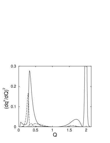
FIG. 33.: The change of the non-collective coordinates with the collective coordinate, which are related to $D$ as discussed in the text. The solid line represents the second coordinate (in harmonic frequency), the dashed the third.

FIG. 34.: The change of the moments of inertia along the collective path. The solid line represents the moment of inertia around the $z$-axis, the long-dashed around the $y$ one, and the dashed around the $x$.

To complete the discussion of parameters of the Hamiltonian we have also calculated the moments of inertia, using the approach in Sec. IV D 4. These are displayed in Fig. 34. The moments of inertia behave relatively smoothly (although they do not follow the irrotational pattern). Where $D$ has its largest value the moments of inertia seem to change least smoothly.

FIG. 35.: The square of the wave function for the four lowest $0^{+}$ eigenstates. The solid line is the lowest, the long-dashed the second, the short-dashed the third and the dashed dotted the fourth state.

Though we have found that decoupling is not good everywhere, we have nevertheless used the Hamiltonian we have constructed,

$${\cal H}=\mbox{$\frac{1}{2}$}\sum_{i}\frac{J_{i}^{2}}{{\cal I}_{i}}+\mbox{$\frac{1}{2}$}P^{2}+\bar{V}(Q),$$ (335)

to generate spectra and compare to the full shell-model calculation in the $sd$ model space. To that end we need to requantize the Hamiltonian (335). Since we are working in the intrinsic system we have to be very careful. The necessary symmetry properties were, in effect, set out a long time ago by Bohr [87] and are discussed in Appendix C of Ref. [29], where details of the numerical solution of the Schrödinger equation for the Hamiltonian (335) are also given. The only thing that needs to concern us here is that we decompose the eigenfunctions as

$$\phi(Q\Omega)_{IMa}=\sum_{K}\phi_{IKa}(Q)\langle\Omega|IMK\rangle,$$ (336)

where $\langle\Omega|IMK\rangle$ are appropriately symmetrized angular functions, the $K$ summation only runs over positive and even values, and $K=0$ is excluded for odd $I$. Using these ideas it is not very hard to write down a finite difference representation for the Hamiltonian matrix which in its turn can be diagonalized in order to obtain eigenvalues and eigenfunctions. In Fig. 35 we give the eigenfunctions for the states with zero angular momentum. The ground state can not be very sensitive to the badness of decoupling, since it is very small for $Q>1$, but the first and other excited states have sizable values in the region of bad decoupling. This means that we do not believe that the corresponding eigenvalues are very good approximations to the shell model values. If we look at the spectrum as given in Fig. 36, we indeed see that the ground state rotational band is reproduced quite well. The band built on the oblate minimum (the second $0^{+}$ state), comes at much too low an excitation energy. Again the moment of inertia of that band is more or less correct. The other $0^{+}$-states also come out at a lower energy than their shell-model counterparts. Further note the $3^{+}$ state that is found to lie at too high an excitation energy. This is probably partially due to the neglect of odd multipoles in our calculation, which certainly would lower the energy of such a state, but this question requires further study.

FIG. 36.: The spectrum calculated from a requantization of the collective Hamiltonian,

Let us now study how quantum corrections to the potential energy alter this picture. We write

$$\bar{V}(Q)=\bar{V}_{0}(Q)+\mbox{$\frac{1}{2}$}\left[\sum_{a}\omega_{a}-\mbox{Tr}(A)\right]-\left[(H_{11})^{(0)}+(H_{04}+H_{40})^{(0)}\right]-\sum_{i}\frac{\langle J_{i}^{2}\rangle}{2{\cal I}_{i}}.$$ (337)

The first two corrections terms are the ones described in the previous section and do not need further explanation apart from the statement that we use only the ellipsoidal excitations to calculate these two terms; the last term, which is a subtraction of the expectation value of the rotational energy in the local Hartree-Fock state, is just a part of the total expression for the quantum corrections obtained from the remaining three quarters of the space (see, e.g., Ref. [6], Eq. (8.111)).

The quantum corrected potential energy is given in Fig. 31 as the dashed line. Clearly we have deeper minima and a higher barrier, so that the wave functions will become more strongly localized on the minima. In Fig. 37 we give each of the corrections to the potential energy separately. The solid line represents the quasiboson result $\mbox{$\frac{1}{2}$}(\sum_{a}\omega_{a}-\mbox{Tr}({\cal A}))$, the long-dashed line represent the rotational energy $-\sum_{\i}{\langle J_{i}^{2}\rangle}/{2{\cal I}_{i}}$. We have not shown the “overcounting correction” $-[(H_{11})^{(0)}+(H_{04}+H_{40})^{(0)}]$. We find that to good approximation this equals zero, a result that can be shown to become exact in the perturbation limit. We do not understand why this relation holds so well for our calculation, but it may be due to a weak residual interaction. In any event, in the following we shall disregard this term because of its small contribution, and concentrate on the two remaining terms.

FIG. 37.: The quantum corrections to the potential. The solid line is the RPA correction, and the dashed line the rotational energy correction.

TABLE III.: A comparison of various approximate calculations of the $0^{+}$ energies. $E_{\mu}$ gives absolute energies, whereas $E^{x}_{\mu}$ represents the excitation energies. The first column gives the exact shell-model results. The next two column represent the results of quantization of the one-dimensional collective Hamiltonian; the first without quantum corrections, and the second with inclusion of these corrections. The column labeled “2D” gives the results of the approximate two-dimensional calculation discussed in the text. The last column gives the results obtained from the RPA on either minimum.

	shell model	1D		2D	RPA
		no zero pt	zero pt
$E_{0^{+}_{1}}$	-149.638	-140.535	-146.941	-146.904	-147.556
$E_{0^{+}_{2}}$	-145.121	-137.580	-141.987	-142.163	-142.381
$E_{0^{+}_{3}}$	-140.409	-132.822	-134.929	-138.134	-138.256	(138.058)
$E_{0^{+}_{4}}$	-139.634	-127.841	-130.858	-137.347	-136.618	(136.187)
$E^{x}_{0^{+}_{2}}$	4.517	2.954	4.953	4.741	5.175
$E^{x}_{0^{+}_{3}}$	9.229	7.712	12.012	8.670	9.300	(9.498)
$E^{x}_{0^{+}_{4}}$	10.004	12.693	16.091	9.557	10.937	(11.369)

In Table III we give the numerical values we have calculated for some low-lying $0^{+}$ states. We both give absolute and excitation energies to show the effects of various approximation schemes in the best possible way. The first column gives the exact shell model result, as a benchmark to measure the quality of various approximations. The second and the third column give the results of a requantization of the one-dimensional Hamiltonian without (second column) and with (third column) the inclusion of quantum corrections. Not surprisingly the absolute value for the energies becomes closer to the true value if we include quantum corrections, even though we apparently still need more to attain the correct result. It is gratifying to see that the excitation energy of the first excited $0^{+}$-state, the band head of the first excited band, is much closer to the true value.

For the sake of comparison we give the RPA value for the oblate and prolate minima, which are $V(Q)+\frac{1}{2}\omega_{1}$, as well as the excitations obtained by adding $\omega_{1}$ (or $\omega_{2}$) to this value. As can be seen $\omega_{1}$ and $\omega_{2}$ are quite close. This has to do with the fact that we should really use two collective coordinates. Stopping short of that approach we have done a poor man’s calculation along the collective path. To each point we assign two coordinates $(Q_{1},q_{2})$ where $Q_{1}$ is the $Q$ used previously and $q_{2}$ is the result of summing the numbers $\Delta Q_{2}$ defined in Sec. IV D 5 in our discussion of the goodness of decoupling. We then requantize an approximation to the Hamiltonian (valid for $0^{+}$-states alone), that includes the second collective coordinate in an harmonic approximation only,

$$H = \mbox{$\frac{1}{2}$}(P_{1}^{2}+P_{2}^{2})+E_{\rm HF}(Q^{1})+\mbox{$\frac{1}{2}$}\omega_{2}^{2}(Q^{2}-q^{2}(Q^{1}))^{2}$$ (339)

$$+\mbox{$\frac{1}{2}$}\sum_{a>2}\omega_{a}-\mbox{$\frac{1}{2}$}\mbox{Tr}[{\cal A}(Q^{1})]-\mbox{$\frac{1}{2}$}\sum_{j}\langle J^{2}_{j}\rangle/{\cal I}_{j}(Q^{1}).$$

The results of this calculation are given in the column labeled ‘2D’ and can be seen to give a much better overall result for the excitation spectrum.

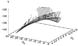
FIG. 38.: A representation of the two-dimensional potential energy surface for ²⁸Si using lines that “slice” through the surface.

A full 2D calculation has proven to be a major problem. The first reason for this is that it was not obvious how to construct a stable algorithm. Using the path-following approach that we have applied to find the valley, it was realized that the best approach we could imagine was to calculate slices through the two-dimensional surface, starting from points on the valley. We chose to use the constraint that $-1/2(Q_{0}-q_{0})=\sqrt{3/8}(Q_{2}-q_{2})$, where $q_{0}$ and $q_{2}$ are the quadrupole coordinates on the valley floor. Unfortunately the path-following algorithm using local coordinates is not as stable as the standard form of PITCON, and we encounter some failures, but these can probably be patched up. The real problem is the structure of the surface. As can be glanced from Fig. 38, the structure is quite complex. An even more quantitative feel can be obtained from Fig. 39, where we show both the first few slices (lower panel), and a bifurcation-like change in the character of the surface (upper panel). We have stopped each line calculation when the density matrix becomes axial, since then we can continue the potential surface by reflection around the $z$-axis. Note that this is stronger than the condition $\gamma=n\pi/3$, since a state can be triaxial with an axial quadrupole moment. Indeed, in the calculations near the HF minimum we see, apart from lack of convergence in some cases, that we do find states that have axial quadrupole moments, but are not axial. We also note that these slices end up on two different axial points. This suggests, and this is also seen in a calculation for axial deformation only, that the bottom of the potential surface looks somewhat like the bottom of a paraboloid, very different from what we would expect.

FIG. 39.: A combination of a few slices through the potential energy surface. The lower panel is near the HF minimum, the upper panel show a reconnection phenomenon about midway through the valley.

Equally worrisome is the behavior in the middle of the path, where we find what looks like an avoided crossing between two intersection surfaces becoming a funnel (i.e., the surfaces touch), after which the surfaces reconnect in a different way. This is a difficult problem to deal with computationally.

Clearly the potential energy surface found does not lend itself easily to a quantization procedure, even if we fix the convergence problems with the algorithm. This points at the weakest point in this model study, the fact that effective interactions in small model spaces must be extremely complicated to describe the full dynamics. Such interactions should not naturally lead themselves to a collective approach, and that is a large source of the difficulties.

We have, however, shown that we can construct a one-dimensional path that gives a reasonable description of the lowest states in ²⁸Si. Inclusion of the quantum corrections in our calculation for ²⁸Si improves the calculation of both binding and excitation energies. We have shown that a quasi two-dimensional calculation improves the results even more.

E A basis for self-consistent cranking operators

In the usual Hartree-Fock or Hartree-Fock-Bogoliubov calculations which are being used to study deformed and superdeformed nuclei as well as fission [88, 89, 90], the multidimensional surface is generated by cranking, using some one-body operators to move away from the local minima. The most commonly employed constraint operators are just the multipole spherical harmonics. Despite some apparent successes of such calculations, the procedure is far from being satisfactory [91], both from the theoretical and practical points of view. One may indeed raise the following questions:

1. Even though the quadrupole $L=2$ mode seems to play a dominant role in the deformation of nuclei, there is no reason to limit oneself to this or other space-dependent cranking operators. Spin-dependent components may not be negligible. Furthermore, the radial structure may turn out to be much more complicated than the simple $r^{L}$ form of the electric multipole operators.

2. In order to cover the space of the collective motion, it is most probable that one is required to use a large number of these operators, should they not be well chosen. For heavy nuclei, a calculation with many (three or more) cranking operators is impracticable. One therefore must wonder whether it is possible to cover the space of the collective motion by choosing a small set of operators that are well-defined linear combinations of elementary ones. A positive answer to this question would be of significant value for the study of heavy nuclei.

In this section we analyze a few aspects of these questions. Section IV E 1 shows what we can learn from the case of the Silicon nucleus [33]. The more interesting study of the Baranger-Kumar pairing-plus-quadrupole model is described in Sec. IV E 2 [40, 41]. The account of a model study that follows in Sec. IV F also bears on this subject.

1 Self-consistent cranking operators for the ${}^{28}Si$ nucleus

The Kuo interaction used for the study of this nucleus is very complex. Aside from the space structure, it also depends on spin and isospin. It is therefore reasonable to expect that the cranking operator reflects these degrees of freedom as well. As a first study, let us neglect the isospin, which is reasonable for this light $N=Z$ nucleus. We shall choose the following two sets of one-body operators: the usual set of spin-independent multipole operators

$$\hat{o}^{S=0}_{J\Sigma}=F_{J}(r)Y_{J\Sigma}(\hat{r})$$ (340)

and the spin-dependent operators

$$\hat{o}^{S=1}_{LJ\Sigma}=F_{LJ}(r)[S\times Y_{L}]_{J\Sigma}$$ (341)

where $S$ is the spin operator and $F(r)$ represents a radial dependence.

To see whether the cranking operator, the chosen collective solution of the RPA equation (247) can be expressed in terms of the above sets of operators, we shall calculate it in two ways:

1. We first solve the original p-h RPA equation to get a set of p-h matrix elements $f_{ph}$. These are properly normalized.

2. Next, we solve the projected RPA equation according to the method given in Sec. IV A 5 over the above sets of operators. This gives a new set of p-h matrix elements $\bar{f}_{ph}$.

The criteria for good projection is the smallness of the following quantity

$$\delta = \sum_{ph,p^{\prime}h^{\prime}}f_{ph}B^{ph,p^{\prime}h^{\prime}}(f_{p^{\prime}h^{\prime}}-\bar{f}_{p^{\prime}h^{\prime}})$$ (342)

$$= 1-f_{ph}B^{php^{\prime}h^{\prime}}\bar{f}_{p^{\prime}h^{\prime}},$$ (343)

where we have used the normalization imposed in Eq. (303). In view of the chosen normalization, $0<\delta<1$ with $\delta=0$ corresponding to exact projection and $\delta=1$ to the case where the two solutions are orthogonal.

Let us limit our study to just one point on the collective path, namely at the HF minimum: It is at this point that the number of operators required is the smallest, while at the same time it is sufficient for the stated purpose.

TABLE IV.: The energy of the collective state and the value of the representation measure $\delta$ when more and more elementary operators are added.

$J$	$S$	$L$	$\Omega$	$\delta$
2	0	2	10.531	0.7383
4	0	4	10.592	0.6852
2	1	2	6.860	0.1572
3	1	2	6.631	0.1226
3	1	4	6.631	0.1226
4	1	4	6.034	0.0000

First of all, we assume that the model space consists of just the $sd$-shell, as given in Sec. IV D above. In this case, the radial dependence is irrelevant, as explained below. Table IV gives the results for the quantity $\delta$ defined above together with the energy $\Omega$ of the collective state obtained when more and more operators are added to the operator basis (in going from one line to the next in the table). It is seen that the spin-independent operators alone are far from being sufficient to represent the RPA cranking operator. Even after having exhausted all the available values of $J$ compatible with the model space, $\delta$ is still found to have a large value of $0.6852$ and $\Omega=10.59$ MeV is still much larger than the value obtained by direct diagonalization of the RPA equation which is $\Omega=6.034$. It turns out that the spin-dependent part ( $S=1$ ) is very important, much more important than the spin-independent one. As a matter of fact, by including all the given operators, one can show that the basis is complete and thus gives an exact ($\delta=0$) representation of the self-consistent cranking operator. The possibility of an exact representation of $f$ in this case also means that there is no need to consider a more complicated radial form factor $F(r)$. This is so because the average value of $r^{k}$ is the same for any state of the model space and changing $k$ just adds an overall factor which can be absorbed in the normalization.

TABLE V.: The smallest value $\delta_{min}$ obtained when the model space is enlarged sequentially for three choices of the radial form factor $F(r)$.

Model	$F(r)=r^{2}$	$F(r)=$	$\rho(r)r^{2}$
space		$r^{2}+r^{4}$
+ $2s_{1/2}$	0.00	0.00	0.00
+ $1d_{3/2}$	0.0345	0.00	0.00
+ $1d_{5/2}$	0.1986	0.0011	0.1375
+ $0g_{7/2}$	0.2473	0.0932	0.1206
+ $0g_{9/2}$	0.5146	0.4132	0.3644

To see whether more complicated form factors may be necessary, we shall enlarge the model space to include, in addition to the $sd$-shell, the next positive parity $sdg$-shell. By adding the different subshells one by one into the model space and trying to get the best representation, it is found that a single r-dependence of the form $r^{k}$ is no longer sufficient. Table V shows the best ( the smallest ) $\delta$ , denoted $\delta_{min}$, obtained when the model space is enlarged successively: $\delta_{min}$ increases from zero to $0.5146$ when all the $sdg$-shell is included. Recalling that $\delta_{min}$ corresponds to including all the available angular momenta and spins so that, to improve the result, the only remaining possibility is an additional radial dependence. As a matter of fact, adding another radial dependence of the form

$$F(r)=r^{k}G(r)$$ (344)

leads to much better results, as shown in the third column of Table V. These results have been obtained with $k=2$ and $G(r)=r^{2}$, that is with two radial form factors $r^{2}$ and $r^{4}$. It looks as if an additional $r$ dependence is needed every time one adds a new shell, with the consequence that the number of elementary operators is doubled each time. Of course, this is undesirable. One would like to limit as much as possible the number of elementary operators for computational reasons. It has been found that the radial form factor

$$F(r)=\rho(r)r^{2}$$ (345)

where $\rho(r)$ is the average density, allows a better fit of the cranking operator than $r^{2}$ alone and gives results comparable to those found by using two independent radial form factors (see the last column of Table V). The attractive feature of the above form is that it allows an automatic cutoff of the unbounded nature of $r^{2}$ and its wild behavior when a large number of harmonic oscillator states is used in the calculation.

In conclusion, the theory allows the determination of a self-consistent cranking operator that is expressible in terms of linear combination of elementary one-body operators. For the study of heavy nuclei for which the construction of the complete particle-hole RPA matrix and its diagonalization may become prohibitive, the knowledge of a limited set of basis operators provides a practical way to solve the problem. The result constitutes a considerable improvement over the current practice based on fixed cranking operators.

2 Cranking operators in the Pairing-Plus-Quadrupole Model

The P+Q model is probably one of the most simple and successful nuclear Hamiltonians that allows us to discuss realistic problems involving pairing and quadrupole degrees of freedom. Baranger and Kumar analyzed in great detail the (adiabatic) collective motion in the P+Q model assuming that the collective variables are the mass quadrupole operators [1, 2, 3, 4, 5]. Thus, they reduced the large number of two-quasiparticle (2qp) degrees of freedom (of the order of thousands) into only two collective coordinates, $\beta$ and $\gamma$. However, a previous study of the $O(4)$ model [37] suggests that even for this simple Hamiltonian, the self-consistent collective coordinate is not as trivial as it seems to be. We show below that the normal-mode coordinate of the random-phase approximation (RPA) is quite different from the mass quadrupole operator. This is especially true when the system is deformed.

For simplicity, let us assume that we are at the HFB minimum. At this point, the local RPA is equivalent to the quasiparticle RPA with the constrained Hamiltonian

$$H^{\prime} = H-\sum_{\tau=n,p}\lambda_{\tau}N_{\tau},$$ (346)

$$H = \sum_{k}\epsilon_{k}c_{k}^{\dagger}c_{k}-\sum_{\tau=n,p}\frac{G_{\tau}}{2}\left(P_{\tau}^{\dagger}P_{\tau}+P_{\tau}P_{\tau}^{\dagger}\right)-\frac{\chi}{2}\sum_{K=-2}^{2}Q_{2K}^{\dagger}Q_{2K}$$ (347)

$$= \sum_{k}\epsilon_{k}c_{k}^{\dagger}c_{k}-\frac{1}{2}\sum_{\sigma}\kappa_{\sigma}R_{\sigma}R_{\sigma}+\frac{1}{2}\sum_{\sigma}\kappa_{\sigma}S_{\sigma}S_{\sigma},$$ (348)

where $\epsilon_{k}$ are spherical single-particle energies and $N_{\tau}=\sum_{k\in\tau}c_{k}^{\dagger}c_{k}$ are the number operators for neutrons ($\tau=n$) and protons ($\tau=p$). The operators $R_{\sigma}$ and $S_{\sigma}$ are the hermitian and anti-hermitian components, respectively, of the pairing operators, $P_{\tau}^{\dagger}=\sum_{k\in\tau,k>0}c_{k}^{\dagger}c_{\bar{k}}^{\dagger}$, and the dimensionless quadrupole operators, $Q_{2K}=b_{0}^{-2}\sum_{kl}\langle k|r^{2}Y_{2K}|l\rangle c_{k}^{\dagger}c_{l}$, where $b_{0}=(\hbar/m\omega_{0})^{1/2}$ is the harmonic oscillator length. The Hamiltonian contains five operators of $R_{\sigma}$-type and four of $S_{\sigma}$-type. Together with the corresponding coupling constants $\kappa_{\sigma}$,

$$\begin{array}[]{ccccccc}R_{\sigma}&=&(P_{+}^{(+)})_{n},&(P_{+}^{(+)})_{p},&Q^{(+)}_{20},&Q^{(-)}_{21},&Q^{(+)}_{22},\\ S_{\sigma}&=&(P_{-}^{(+)})_{n},&(P_{-}^{(+)})_{p},&&Q^{(+)}_{21},&Q^{(-)}_{22},\\ \kappa_{\sigma}&=&G_{n},&G_{p},&\chi,&\chi,&\chi,\end{array}$$ (349)

where

$$(P_{\pm}^{(+)})_{\tau} = \frac{1}{\sqrt{2}}(P_{\tau}\pm P_{\tau}^{\dagger}),\quad\mbox{ for }\tau=n,p,$$ (350)

$$Q^{(\pm)}_{2K} = \frac{1}{\sqrt{2}}(Q_{2K}\pm Q_{2-K}),\quad\mbox{ for }K=0,1,2.$$ (351)

The $(\pm)$ superscripts indicate the signature quantum number, $e^{-i\pi J_{x}}o^{(\pm)}e^{i\pi J_{x}}=\pm o^{(\pm)}$. Following the standard formulation of the model, we shall neglect the Fock terms, the contributions of the pairing force to the Hartree potential and those of the quadrupole force to the pairing potential.

Utilizing the procedure outlined in Sec. IV A, and illustrated in Sec. IV E 1, one arrives at the classical Hamiltonian

$$\mbox{$\cal H$}\equiv\langle\Psi|H|\Psi\rangle\approx E_{0}+\frac{1}{2}B^{\alpha\beta}\pi_{\alpha}\pi_{\beta}+\frac{1}{2}V_{\alpha\beta}\xi^{\alpha}\xi^{\beta}\ ,$$ (352)

in terms of the canonical variables $(\xi,\pi)$. Here, each of the indices ($\alpha,\beta,\cdots$) indicates a pair of 2qp indices ($ij,kl,\cdots$). The mass and curvature parameters are explicitly given by

$$B^{\alpha\beta} = E_{\alpha}\delta_{\alpha\beta}+2\sum_{\rho}\chi_{\rho}S^{(\rho)}_{\alpha}{S^{(\rho)}_{\beta}}\ ,$$ (353a)

$$V_{\alpha\beta} = E_{\alpha}\delta_{\alpha\beta}-2\sum_{\rho}\chi_{\rho}R^{(\rho)}_{\alpha}{R^{(\rho)}_{\beta}}\ ,$$ (353b)

where $E_{\alpha}$ are the Hartree-Bogoliubov quasi-particle energies. Following Ref. [1, 2, 3, 4, 5], we multiply the quadrupole operators by a factor $\alpha_{\tau}^{2}$ with $\alpha_{n}=(2N/A)^{1/3}$ and $\alpha_{p}=(2Z/A)^{1/3}$, and also reduce the quadrupole matrix elements between the states of the upper shell by a factor $\zeta=({\cal N}_{\rm L}+\frac{3}{2})/({\cal N}+\frac{3}{2})$, where ${\cal N}$ is the oscillator quantum number operator and ${\cal N}_{\rm L}$ is the number of quanta in the lower shell. Thus, the modified quadrupole operators are defined as $Q_{2K}\equiv(Q_{2K})_{n}+(Q_{2K})_{p}$, with $(Q_{2K})_{n}=\alpha_{n}^{2}\zeta(r^{2}Y_{2K})_{n}$ and $(Q_{2K})_{p}=\alpha_{p}^{2}\zeta(r^{2}Y_{2K})_{p}$ (which we shall refer to as “the quadrupole operators”).

Recalling that we are studying only the HFB minimum, the solution of t he RPA equation

$$V_{\alpha\gamma}B^{\gamma\beta}f^{\mu}_{,\beta}=(\Omega^{\mu})^{2}f^{\mu}_{,\alpha}\ ,$$ (354)

which involves the diagonalization of the RPA matrix $V_{\alpha\gamma}B^{\gamma\beta}$ whose dimension is equal to the number of active 2qp degrees of freedom. For separable forces, this can be simplified by solving a dispersion relation, which facilitates the numerical calculations for heavy nuclei. In general, however, the RPA diagonalization requires extensive computational resources. Now let us approximate an eigenvector using a selected set of one-body operators $\{\hat{o}^{(i)}\}$:

$${f}_{,\alpha}=\sum_{i}c_{i}o^{(i)}_{\alpha}\ ,$$ (355)

where $o^{(i)}_{\alpha}$ indicate the 2qp matrix elements of operator $\hat{o}^{(i)}$. Then, instead of the full RPA equation (354), we obtain a projected RPA equation

$${M}^{ij}C^{n}_{j}=\left(\bar{\Omega}^{n}\right)^{2}\bar{O}^{ij}C^{n}_{j}\ ,$$ (356)

see Eqs. (298a-298c). The dimension of ${M}^{ij}$ and ${O}^{ij}$ is equal to the number of selected one-body operators $\{\hat{o}^{(i)}\}$. Therefore, if we can approximate the RPA eigenvectors by using a small number of operators, it will significantly reduce the computational task.

A criterion for good projection may be given by the closeness of the projected RPA frequencies $\bar{\Omega}$ to the real RPA frequencies $\Omega$. Another criterion is the smallness of the quantity $\delta$, defined as in Eq. (343).

The theory has been applied to several heavy isotopes. Here we report the numerical results for even-even Sm isotopes (A=146$\sim$154). The form of the P+Q model is that discussed in the second and third of the series of papers by Baranger and Kumar [3, 4]. The model space and the parameters, such as the spherical single-particle energies, the pairing and quadrupole force strengths, are taken from Table 1 in the third paper. The equilibrium parameters ($\beta$, $\gamma$, $\Delta$, $\lambda$) are found to agree with Table 2 of the same paper. The ground states of ^146,148Sm are spherical ($\beta=0$) and the others have prolate shapes ($\beta>0,\gamma=0$).

FIG. 40.: Calculated excitation energies of quadrupole, $\beta$ and $\gamma$ vibrations for even-even Sm isotopes. Note that the ground states of ^146,148Sm are spherical. The closed circles indicate the RPA results while the open symbols are the results of projected RPA calculations. See the main text for the difference between (1), (2) and (3).

Figure 40 shows the excitation energies (RPA frequencies) of $\beta$ and $\gamma$ vibrations, obtained by the RPA and projected RPA calculations. For the projected RPA calculations, we have adopted three different sets of one-body operators. The first and simplest choice is to use the operators appearing in the separable forces, the pairing and quadrupole operators, $P_{\tau}$, $P_{\tau}^{\dagger}$, $(Q_{2K})_{\tau}$ ($\tau=n,p$). This choice is denoted as (1) in the figure. In this case the projected RPA matrices of Eq. (298a) are two dimensional for spherical nuclei and for $\gamma$ vibrations, while they are six dimensional for the $\beta$ vibrations. The calculated frequencies are $7\sim 8$ MeV which are $5\sim 6$ MeV larger than the corresponding RPA frequencies. In the second set, labeled as (2), we increase the number of operators. We keep both the pairing and quadrupole operators, but include two additional quadrupole operators with “monopole” radial dependence, $(r^{0}Y_{2K})_{\tau}$. We also include the hexadecapole operators, $(r^{4}Y_{4K})_{\tau}$, and the rank-2 spin-dependent operators, $([r^{0}Y_{2}\times{\mathbf{s}}]^{(2)}_{K})_{\tau}$, $([r^{2}Y_{2}\times{\mathbf{s}}]^{(2)}_{K})_{\tau}$. As far as the frequencies are concerned, we can see some improvement over the case (1) for spherical and the $\gamma$ vibrations in deformed nuclei, though they are still much higher than the real RPA frequencies. For the $\beta$ vibrations, the inclusion of the additional rank-2 (and higher rank) operators seems not so important. Actually we see that the $\beta$ vibrations are found to have a significant amount of monopole components. For the last set, denoted as (3), we adopt the same operators as (1) but each 2qp matrix element is weighted with a factor $(E_{\rm 2qp})^{-2}$. This means that we employ a set of state-dependent one-body operators $\{\widetilde{o}^{(i)}\}$ defined by

$$\widetilde{o}\equiv\sum_{\alpha}\frac{o_{\alpha}}{(E_{\alpha})^{2}}(a^{\dagger}a^{\dagger})_{\alpha}+\mbox{h.c.}\ .$$ (357)

The result of this projection is now almost identical to that of the full RPA.

TABLE VI.: Calculated values of $\delta$, Eq. (343), of the projected RPA solutions for Sm isotopes. The columns (1), (2), (3), (1-a) and (1-b) represent the different projections (see text). For the spherical nuclei (^146,148Sm), there is no distinction between $\beta$ and $\gamma$ vibrations.

	$\beta$ vibration					$\gamma$ vibration
A	(1)	(1-a)	(1-b)	(2)	(3)	(1)	(1-a)	(1-b)	(2)	(3)
146	0.271	0.132	0.225	0.421	0.009
148	0.243	0.131	0.184	0.314	$3\times 10^{-4}$
150	0.602	0.499	0.519	0.632	0.026	0.610	0.342	0.507	0.685	0.092
152	0.497	0.346	0.433	0.526	0.020	0.616	0.279	0.472	0.691	0.081
154	0.513	0.117	0.437	0.534	0.002	0.636	0.208	0.426	0.679	0.052

In Table VI, the quality of projection $\delta$, Eq. (343), is listed. In the cases (1) and (2), where the RPA vectors are projected on the elementary operators, $\delta\gtrsim 0.25$ for ^146,148Sm and $\delta\gtrsim 0.5$ for the others. Therefore, roughly speaking, selected one-body operators possess at most 75% (50%) of overlap with the real eigenvectors in spherical (deformed) nuclei. On the other hand, the projection (3) exhausts more than 90% of real eigenvectors even for the worst case. At first sight it may look strange that $\delta$ is larger for (2) than for (1), while the energy for (2) is lower. This is due to the fact that case (2) is dominated by certain neutron components. Since the relevant neutron 2qp energies are lower than those of protons, this proton-neutron asymmetry leads to a decrease in the frequency $\bar{\Omega}$ and at the same time an increase in $\delta$. This is also a reflection of the poor quality of the approximation.

Figure 40 and Table VI indicate that it is very difficult to obtain sensible results by using elementary one-body operators (i.e., of the form (1) or (2)). This is mainly due to the fact that the RPA eigenvectors, when being projected onto elementary one-body operators, have unrealistically large amplitudes for high-lying 2qp components. In order to demonstrate this, we introduce a cut-off energy $\Lambda_{\rm cut}$ for the 2qp matrix elements, i.e., $o^{(i)}_{\alpha}=0$ for $E_{\alpha}>\Lambda_{\rm cut}$. We then perform the projected RPA calculation with the truncated one-body operators from set (1). The resulting values $\delta$ are listed in Table VI for $\Lambda_{\rm cut}=5$ MeV (1-a) and for 10 MeV (1-b). We see that the major contributions to the RPA modes come from the 2qp components with $E_{\rm 2qp}<5$ MeV. We thus conclude that the superiority of the projection (3) simply comes from its being capable of suppressing the unnecessary high-energy components by the factor $(E_{\rm 2qp})^{-2}$.

This suppression factor is not arbitrary, but can be derived from the following simple argument. If we have a single-mode separable force $H=-(1/2)\chi RR$ (assuming no coupling among different modes), we can determine the RPA eigenvectors analytically, $f^{\mu}_{,\alpha}\propto R_{\alpha}/((E_{\alpha})^{2}-(\Omega^{\mu})^{2})$. In the limit that $\Omega^{\mu}\ll E_{\rm 2qp}$, the projection on $f_{,\alpha}\propto R_{\alpha}/(E_{\alpha})^{2}$ gives the exact answer. It is worth noting that taking $R=Q_{22}$, we find exactly the formula for $\gamma$ vibrations as discussed in the first paper of Baranger and Kumar [1].

Let us examine the projection (3) in more detail. For spherical Sm nuclei, the RPA eigenvector has a good isoscalar character and can be approximated as $\bar{f}\approx(\widetilde{Q}_{2})_{n}+(\widetilde{Q}_{2})_{p}$ where the tilde indicates that the matrix elements include the suppression factor as in Eq. (357). For deformed nuclei, where the collectivity of the vibrational states is smaller than for spherical nuclei and the pairing modes can mix with the quadrupole ones, the situation is more complex. Taking ¹⁵⁴Sm as an example, the eigenvectors of $\beta$ and $\gamma$ vibrations are

$$\bar{f}^{\beta{\rm-vib}} = (\widetilde{Q}_{20})_{n}+0.91(\widetilde{Q}_{20})_{p}-0.48\widetilde{P}_{n}-0.44\widetilde{P}_{p}+0.085\widetilde{P}_{n}^{\dagger}-0.14\widetilde{P}_{p}^{\dagger}\ ,$$ (358a)

$$\bar{f}^{\gamma{\rm-vib}} = (\widetilde{Q}_{22})_{n}+0.87(\widetilde{Q}_{22})_{p}\ .$$ (358b)

For the $\beta$ vibration, we find a significant mixing with the monopole (pairing) modes.

In conclusion, we have examined the possibility of expressing the self-consistent cranking operator in terms of a limited set of one-body operators. It seems very difficult to approximate the normal-mode vectors with use of elementary one-body operators. This difficulty disappears, however, when we use a small number of state-dependent one-body operators. This may reflect the importance of the self-consistent determination of the collective coordinates for large amplitude collective motion, because the coordinates now have a strong state-dependence as well. The structure of the self-consistent cranking operators is clearly changing when we move from spherical to deformed nuclei. For the study of large amplitude collective motion in heavy nuclei for which the diagonalization of the RPA matrix becomes too time-consuming, the results obtained here may give a hint for a correct choice of a state-dependent basis of operators. The choice of a limited set of (state dependent) basis operators provides a practical way to solve the LHA through the projection. With the self-consistent cranking operators, the LHA should provide a significant improvement over the conventional CHFB calculation based on fixed cranking operators.

F A model study of shape transitions and shape coexistence

1 Introduction

Clearly one of the most important aspects of heavy nuclear systems is the role of the pairing interaction, which needs to be tackled within the framework of our theory. In a first application [36], that we shall not reproduce here, we applied the LHA to analyze properties of collective motion in a semi-microscopic model of nucleons interacting through a pairing force, coupled to a single harmonic variable giving a macroscopic description of the remaining degrees of freedom. It turned out that with this method the system automatically selects either diabatic (shape coexistence) or adiabatic collective surfaces according to the strength of the pairing interaction. However, we felt that it would be beneficial to study a fully microscopic Hamiltonian.

To this end we investigate the collective motion in a model which describes a system of nucleons interacting through a simplified version of the pairing-plus-quadruple force [92]. Although the Hamiltonian has a very simple form, we shall see that the model can reproduce the qualitative features of many kinds of interesting situations observed in real nuclei, such as a spherical-to-deformed transition, and nuclei with shape coexistence, where more than one equilibrium shape play a role.

In the case of a single-$j$ shell the model Hamiltonian is built from the generators of an $o(4)$ algebra, which makes exact diagonalization feasible. The model has been originally developed to describe $K^{\pi}=0^{+}$ excitations in deformed nuclei [92], and has also been used as a test-bed for various methods applied to the calculation of collective excitations such as the boson expansion method [93, 94], the selfconsistent collective coordinate method [95], and a semiclassical method [96, 97]. The model can be generalized to multiple shells, where it has been used to investigate shape-coexistence phenomena [98]. Finally, a similar model has been used to study the collective mass parameter in finite superconducting systems [99].

Although the low-lying spectra in nuclei are mostly dominated by the quadrupole phonon ($J^{\pi}=2^{+}$) excitations, the anharmonicity of this mode is very important for many nuclei, especially in a shape-transition region, where the nature of the ground-state changes rapidly with particle number. For instance, the even-even Sm isotopes show a typical example of the spherical to deformed shape transition in which the spectrum shows a strong anharmonicity between the spherical ($N\leq 84$) and deformed ($N\geq 90$) nuclei, especially for ^148,150Sm. These phenomena are primarily related to the competition between the monopole and quadrupole interactions among the valence particles outside a closed core. The pairing-plus-quadrupole model was designed to describe this competition and is well able to reproduce the most important aspects of the experimental data (see [100] and references therein). Later the boson expansion method has been applied to the same model (with an additional quadrupole pairing interaction) for the description of the shape transition in the Sm isotopes [101, 102], and shows excellent agreement with the experimental data. Since the $O(4)$ model is very similar to the pairing-plus-quadrupole model, it would be of significant interest to see whether our method of large amplitude collective motion can properly describe the shape transition phenomena in this exactly solvable model.

The importance of shape-coexistence in nuclear physics can be seen from the multitude of theoretical approaches and the amount of experimental data as compiled in the review paper Ref. [103]. An important example can be found in even semi-magic Sn and Pb isotopes, where the ground states are spherical. However, deformed excited $J^{\pi}=0^{+}$ states have been observed at low-excitation energies in many of these nuclei. These excited states are regarded as states associated with proton two-particle-two-hole (2p-2h) excitations across the closed shell. Using the Nilsson picture, which shows down-sloping single-particle levels above the proton closed shell, and up-sloping levels below it, it is possible to assign a configuration of two particles lying on down-sloping levels and two holes on up-sloping levels. The configuration-constrained Nilsson-Strutinsky calculations as performed by Bengtsson and Nazarewicz [104] have suggested that the diabatic potential-energy curve obtained by switching off the interaction between the 2p-2h and the ground-state (0p-0h) configuration gives a more accurate picture than the conventional adiabatic potential energy. This question, whether the nuclear collective potential is adiabatic or diabatic, is quite old, and was originally raised by Hill and Wheeler [105]. It is our aim to investigate in the $O(4)$ model whether the method is able to provide us with useful information about shape mixing, and to test whether it makes useful predictions concerning whether the collective potential energy is diabatic or adiabatic.

2 Formalism: removal of spurious modes

We have discussed most of the important aspects of our approach in previous sections. The only point of principle that requires special discussion is the treatment of spurious modes. A typical example is given by the Nambu-Goldstone (NG) mode associated with the violation of particle-number conservation. The general problem was first discussed in Sec. II B 5, where it was pointed out that NG modes can have their origin either in the absence of restoring forces, or (less frequently considered) the occurrence of infinite eigenmasses. In the application to the rotational motion in ²⁸Si, we encountered both cases, and found no basic difficulty dealing with them because they occurred in different symmetry spaces of the local RPA. In the present example, we shall see that the NG mode associated with particle-number violation is of the infinite eigenmass type. Therefore, we first describe a general technique for handling such a case.

For the models to be discussed in the following sections, the modes associated with a change in average particle number are given by a linear combination of coordinates:

$$\tilde{f}^{ng}(\xi)=\sum_{\alpha=1}^{n}c_{\alpha}\xi^{\alpha}\ ,$$ (359)

where $c_{\alpha}$ is a constant. The problem is that this mode leads to a zero eigenvalue of the mass,

$$B^{\alpha\beta}\tilde{f}^{ng}_{,\beta}=B^{\alpha\beta}c_{\beta}=0\ .$$ (360)

This means that we cannot invert the mass matrix. The only sensible way to deal with this is to remove these degrees of freedom from our space, by defining a new set of coordinates, $\tilde{\xi}^{\mu}=\tilde{f}^{\mu}(\xi)$. These are required to satisfy

$$B^{\alpha\beta}\tilde{f}^{\mu}_{,\beta}\neq 0\ ,\quad \forall\alpha\mbox{ and }\mu=1,\cdots,n-M\ ,$$ for (361)

$$B^{\alpha\beta}\tilde{f}^{\mu}_{,\beta}=0\ ,\quad \forall\alpha\mbox{ and }\mu=n-M+1,\cdots,n\ ,$$ for (362)

where we assume that there are $M$ Nambu-Goldstone modes ($\mu>n-M$). Then, we may formulate the LHA in the space of $n-M$ dimension, $\{\tilde{\xi}^{\mu}\}_{\mu=1,\cdots,n-M}$, in which $\det(B^{\mu\nu})\neq 0$.

$${\cal M}^{\nu}_{\mu}f^{i}_{,\nu}=(\omega^{i})^{2}f^{i}_{,\mu}\ ,$$ (363)

$${\cal M}^{\nu}_{\mu}\equiv\tilde{V}^{,\nu}_{;\mu}=\tilde{B}^{\nu\nu^{\prime}}\tilde{V}_{;\nu^{\prime}\mu}\ ,$$ (364)

where indices $\mu,\nu,\cdots$ run only from 1 to $n-M$. Our aim is to provide a feasible method to calculate this LHA, namely to calculate the mass parameter $\tilde{B}^{\nu\nu^{\prime}}$, potential $\tilde{V}(\tilde{\xi})$, and their derivatives.

The second equation (362) determines tangent vectors of the NG modes. The rest of coordinates $\tilde{f}^{\mu}$ for $\mu=1,\cdots,n-M$ are arbitrary as long as their derivatives are linearly independent of the others. The full Jacobian matrix $\tilde{f}^{\mu}_{,\alpha}$ allows us to define the derivatives of the inverse transformation, $\tilde{g}^{\alpha}_{,\mu}$ as the inverse of $\tilde{f}$,

$$\tilde{f}^{\mu}_{,\beta}\tilde{g}^{\beta}_{,\nu}=\delta^{\mu}_{\nu}\ ,\quad\tilde{f}^{\mu}_{,\beta}\tilde{g}^{\alpha}_{,\mu}=\delta^{\alpha}_{\beta}\ .$$ (365)

Since all $\tilde{f}^{\mu}_{,\alpha}$ are constant (independent of coordinates), all $\tilde{g}^{\alpha}_{,\mu}$ are also constant and the derivatives $\tilde{f}^{\mu}_{,\alpha\beta}$ (or $\tilde{g}^{\mu}_{,\alpha\beta}$) all vanish. This implies that within the NG subspace the connection vanishes, $\Gamma=0$, and the geometric character of the transformation of any tensor is fully determined in the subspace that does not contain the NG modes. One can use this to calculate the new mass parameter and its derivatives as

$$\tilde{B}^{\mu\nu} = \tilde{f}^{\mu}_{,\alpha}B^{\alpha\beta}\tilde{f}^{\nu}_{,\beta}\ ,$$ (366a)

$$\tilde{B}^{\mu\nu}_{,\lambda} = \tilde{f}^{\mu}_{,\alpha}B^{\alpha\beta}_{,\gamma}\tilde{f}^{\nu}_{,\beta}\tilde{g}^{\gamma}_{,\lambda}\ ,$$ (366b)

and the derivatives of the potential as

$$\tilde{V}_{,\mu} = \tilde{g}^{\alpha}_{,\mu}V_{,\alpha}\ ,$$ (367a)

$$\tilde{V}_{,\mu\nu} = \tilde{g}^{\alpha}_{,\mu}\tilde{g}^{\beta}_{,\nu}V_{,\alpha\beta}\ .$$ (367b)

3 The $O(4)$ model

We shall first study the properties of the single-shell $O(4)$ model. We define fermionic operators $c^{\dagger}_{jm}$ and $c_{jm}$ that create or annihilate a particle in the $J_{z}=m$ sub-state. In terms of these operators we define four pairing ($P$, $P^{\dagger}$, $\tilde{P}$, and $\tilde{P}^{\dagger}$) and two multipole operators ($N$ and $Q$) that close under commutation, and generate the algebra $o(4)$,

$$P^{\dagger} = \sum_{m>0}c_{jm}^{\dagger}c_{j\bar{m}}^{\dagger}\ ,\quad\tilde{P}^{\dagger}=\sum_{m>0}\sigma_{jm}c_{jm}^{\dagger}c_{j\bar{m}}^{\dagger}\ ,$$ (368a)

$$N = \sum_{m}c_{jm}^{\dagger}c_{jm}\ ,\quad Q=\sum_{m}\sigma_{jm}c_{jm}^{\dagger}c_{jm}\ ,\quad$$ (368b)

$$\sigma_{jm} = \left\{\begin{array}[]{ll}+1&\mbox{for }|m|<\Omega/2\\ -1&\mbox{for }|m|\geq\Omega/2\end{array}\right..$$ (368e)

Here we need to require that the pair multiplicity $\Omega=j+1/2$ is an even integer in order for the algebra to close. The sign of $\sigma_{jm}$ is chosen so as to mimic the behavior of the matrix elements of the axial quadrupole operator $\langle jm|r^{2}Y_{20}|jm\rangle$, and we shall call $Q$ the quadrupole operator in the remainder of this work, even though it does not carry the correct multipolarity.

As is well-known, the algebra $o(4)$ is isomorphic to $su(2)\oplus su(2)$. This can be made explicit in terms of the quasi-spin operators

$$A_{+} =\frac{1}{2}\left(P^{\dagger}+\tilde{P}^{\dagger}\right)=A_{-}^{\dagger}\ ,\quad A_{0}= \frac{1}{4}\left(N+Q-\Omega\right)\ ,$$ (369a)

$$B_{+} =\frac{1}{2}\left(P^{\dagger}-\tilde{P}^{\dagger}\right)=B_{-}^{\dagger}\ ,\quad B_{0}= \frac{1}{4}\left(N-Q-\Omega\right)\ ,$$ (369b)

which generate two independent $su(2)$ algebras,

$$\left[A_{+},A_{-}\right] = 2A_{0}\ ,\quad\left[B_{+},B_{-}\right]=2B_{0}\ ,$$ (370a)

$$\left[A_{0},A_{\pm}\right] = \pm A_{\pm}\ ,\quad\left[B_{0},B_{\pm}\right]=\pm B_{\pm}\ ,$$ (370b)

$$\left[{A}_{\mu},{B}_{\mu^{\prime}}\right] = 0\ .$$ (370c)

The Hamiltonian of the model is chosen as a simple quadratic form in (some of) the generators of $o(4)$,

$$H=-GP^{\dagger}P-\frac{1}{2}\kappa Q^{2}\ ,$$ (371)

which mimics the pairing-plus-quadrupole model. Even though the Hamiltonian looks simple, it does not have a closed-form solution (it does not have $O(4)$ dynamical symmetry). Nevertheless a numerically exact solution for the Hamiltonian (371) can be obtained by simple diagonalization. To this end one rewrites the Hamiltonian in terms of the quasi-spin operators ${\mathbf{A}}$ and ${\mathbf{B}}$,

$$H=-G\left(A_{+}+B_{+}\right)\left(A_{-}+B_{-}\right)-2\kappa\left(A_{0}-B_{0}\right)^{2}\ .$$ (372)

This Hamiltonian commutes with the total particle number $N=2(A_{0}+B_{0})+\Omega$, and there are no further constants of the motion. The pairing force tends to align the two quasi-spin vectors ${\mathbf{A}}$ and ${\mathbf{B}}$, so as to obtain the maximal pairing matrix elements, while the quadrupole force tends to de-align them (to maximize $(A_{0}-B_{0})^{2}$). In this picture, the non-integrability of the model, as well as the physics described, is related to the competition between the pairing and the quadrupole force. This is identical to a competition between alignment and de-alignment of the quasi-spins.

For a fixed number of particles $N=2n_{0}$, we construct from the vacuum state $|0\rangle$ all states with a constant number of generators $A_{+}$ and $B_{+}$,

$$|n_{0},k_{a}\rangle=\left[\frac{\left(\frac{\Omega}{2}-k_{a}\right)!\left(\frac{\Omega}{2}-n_{0}+k_{a}\right)!}{\left\{\left(\frac{\Omega}{2}\right)!\right\}^{2}k_{a}!\left(n_{0}-k_{a}\right)!}\right]^{1/2}A_{+}^{k_{a}}B_{+}^{n_{0}-k_{a}}|0\rangle\ ,$$ (373)

where $0\leq k_{a}\leq n_{0}$. Finding the eigenvectors of the Hamiltonian now involves a trivial matrix diagonalization in this basis of dimension ($n_{0}+1$).

The mean-field description of the Hamiltonian (372) is most easily based on the use of a product of $su(2)$ coherent states, one for the $A_{\mu}$ sub-algebra, and another for the $B_{\mu}$ one. (This is the transcription of the TDHFB formalism described in general terms in Sec. A 5, and is our only explicit use of this method in the review.) Each of these states is characterized by a complex variable, $z_{a}$ and $z_{b}$ [106]. The time-dependent mean-field dynamics in this parameterization defines the classical Hamiltonian problem to which we shall apply our methodology. We can also parameterize the coherent state with four real angles [96, 97, 106],

$$|z_{a},z_{b}\rangle = \exp\left[z_{a}A_{+}-z_{a}^{*}A_{-}+z_{b}B_{+}-z_{b}^{*}B_{-}\right]|0\rangle\ ,$$ (374)

$$= \left(\cos\frac{\theta}{2}\cos\frac{\chi}{2}\right)^{\Omega/2}\exp\left[\tan\frac{\theta}{2}\exp(-i\phi)A_{+}+\tan\frac{\chi}{2}\exp(-i\psi)B_{+}\right]|0\rangle\ ,$$ (375)

where we have used

$$z_{a}=\frac{\theta}{2}\exp(-i\phi)\ ,\quad z_{b}=\frac{\chi}{2}\exp(-i\psi)\ .$$ (376)

The time-dependent Hartree-Fock Bogoliubov (TDHFB) equations are in this case the classical equations of motion obtained from the stationary condition of the coherent-state action $\delta S=0$, where

$$S[z] = \int^{t}dt\,\langle z_{a},z_{b}|i\partial_{t}-H|z_{a},z_{b}\rangle\ ,$$ (377)

$$= \int^{t}dt\,\frac{\Omega}{2}\left(\dot{\phi}\sin^{2}\frac{\theta}{2}+\dot{\psi}\sin^{2}\frac{\chi}{2}\right)-\int^{t}dt\,\mbox{$\cal H$}(\theta,\chi;\phi,\psi)\ ,$$ (378)

and

$$\mbox{$\cal H$}=\langle z_{a},z_{b}|H|z_{a},z_{b}\rangle\ .$$ (379)

In order to facilitate our work we introduce real canonical variables $\xi^{\alpha}$ and $\pi_{\alpha}$,

$$\xi^{1} = \frac{\Omega}{2}\sin^{2}|z_{a}|=\frac{\Omega}{2}\sin^{2}\frac{\theta}{2}\ ,\quad\xi^{2}=\frac{\Omega}{2}\sin^{2}|z_{b}|=\frac{\Omega}{2}\sin^{2}\frac{\chi}{2}\ ,$$ (380)

$$\pi_{1} = \arg(z_{a})=-\phi\ ,\quad\pi_{2}=\arg(z_{b})=-\psi\ .$$ (381)

Since these variables are canonical, the equations of motion are of Hamiltonian form

$$\dot{\pi}_{\alpha}=-\frac{\partial\mbox{$\cal H$}}{\partial\xi^{\alpha}}\ ,\quad\dot{\xi}^{\alpha}=\frac{\partial\mbox{$\cal H$}}{\partial\pi_{\alpha}}\ ,$$ (382)

where the classical Hamiltonian (379) is the coherent state expectation value of the Hamiltonian rewritten in terms of canonical variables (the explicit form can be found from that of the more general Hamiltonian discussed in the following section, Eqs. (394a-394h), upon substitution of $q_{\alpha}=1$). The adiabatic Hamiltonian is then found by expanding the full Hamiltonian with respect to $\pi$ up to second order, and is defined in Eqs. (395a-395d).

We discuss next the problem of defining a requantization procedure and the consequences of the adiabatic truncation with respect to momentum. The classical limit of the single-$j$ Hamiltonian has two constants of motion: $\mbox{$\cal H$}=E$ and $\langle N\rangle=2\sum_{\alpha}\xi^{\alpha}=N_{0}$. Since the phase space is four dimensional, this implies the complete integrability of the system, and there is a two dimensional torus on which all classical orbits lie. Due to this special feature of this model, one can apply the Einstein-Brillouin-Keller (EBK) quantization condition. This has been done in Refs. [96, 97] and good agreement with the exact results has been obtained for both energy spectra and transition amplitudes. However, it is impossible to extend this quantization method to non-integrable systems like the ones we will discuss in the following sections. We wish to use the same quantization procedure for the simplest form of the model and the more complicated cases discussed later on, and shall turn to our favorite technique first.

After truncation of the Hamiltonian up to second order in momentum, we can define a collective Hamiltonian by evaluating its value for points on the collective space $\Sigma$ which is parameterized by $x^{1}$ and $p^{1}$, since we have chosen $x^{a}=p^{a}=0;a=1,\cdots,n-1$,

$$\bar{\mbox{$\cal H$}}_{\rm col} = \left.\bar{\mbox{$\cal H$}}_{\rm ad}\right|_{\Sigma}=\frac{1}{2}\bar{B}^{11}(x^{1})p_{1}^{2}+\bar{V}(x^{1})\ ,$$ (383a)

$$\bar{B}^{11}(x^{1}) = \sum_{\alpha\beta}f^{1}_{,\alpha}f^{1}_{,\beta}B^{\alpha\beta}\left(\xi^{\alpha}=g^{\alpha}(x^{1},x^{a}=0)\right)\ ,$$ (383b)

$$\bar{V}(x^{1}) = V\left(\xi^{\alpha}=g^{\alpha}(x^{1},x^{a}=0)\right)\ .$$ (383c)

Since the scale of the collective coordinate $x^{1}$ is arbitrary, we choose to normalize $f^{1}_{,\alpha}$ so as to make $\bar{B}^{11}=1$. Subsequently, the Hamiltonian $\bar{\mbox{$\cal H$}}_{\rm col}$ is quantized in this flat space as [36]

$$\hat{H}_{\rm col}=-\frac{1}{2}\frac{d^{2}}{dx^{2}}+\bar{V}(x)\ ,$$ (384)

where we have replaced $(x^{1},p_{1})$ by $(x,p)$.

In order to evaluate the matrix elements of a one-body operator $F$ (either diagonal or transition matrix elements), we first obtain the collective classical representation of the operator $F$, which in keeping with the adiabatic approximation is expanded in powers of momentum,

$$\bar{\cal F}(x,p)=\left.{\cal F}(\xi,\pi)\right|_{\Sigma}=\left.\langle z|F|z\rangle\right|_{\Sigma}=\sum_{i=0}^{\infty}\left.{\cal F}^{(i)}(\xi,\pi)\right|_{\Sigma}=\sum_{i=0}^{\infty}\bar{\cal F}^{(i)}(x,p)\ .$$ (385)

Here ${\cal F}^{(i)}$ is the term of $i$-th order in $\pi$. The function $\bar{\cal F}$ is requantized, by making the replacement $\bar{\cal F}(x,p)\rightarrow\bar{F}(x,\frac{d}{dx})$, at which point one will have to confront the problem of operator ordering between $x$ and $p$. We shall avoid this problem by keeping, invoking once again the assumption of slow collective motion, only the zeroth order term $\bar{\cal F}^{(0)}$. It is an interesting question what the effect of higher order terms will be. This is clearly outside the scope of the present work, and requires further investigation. Fortunately, in the current model, we have no ambiguity for the quadrupole operator $Q$ because ${\cal Q}^{(i)}=0$ for $i\neq 0$. For convenience we denote the classical limit of the quadrupole operator by $q$. The transition matrix elements can thus be calculated by the one-dimensional integral,

$$\langle n^{\prime}|F|n\rangle=\int dx\Psi_{n^{\prime}}^{*}(x)\bar{F}^{(0)}(x)\Psi_{n}(x)\ ,$$ (386)

where $\Psi_{n}$ are the eigenfunctions of the collective Hamiltonian (384),

FIG. 41.: The excitation energies and transition matrix elements $|\langle n-1|Q|n\rangle|$, all in arbitrary units, in the single-$j$ shell $O(4)$ model as a function of the ratio between the strength of the pairing and that of the quadrupole force. The case (a) is a weak quadrupole force, $2\kappa/G=0.079$, (b) a medium sized one, $2\kappa/G=1.63$ and (c) a very strong one, $2\kappa/G=12.7$. We have constrained $G^{2}+(2\chi)^{2}=1$. The three panels give our standard adiabatic quantization (1), the results from the “adiabatic in coordinates” method (2), and the exact results (3).

From the number of coordinates and momenta found (2+2) we see that the configuration space of the single-$j$ shell model is two-dimensional. Since there is a zero mode ($\det(B^{\alpha\beta})=0$) corresponding to the NG mode associated with the particle number violation, one may obtain a one-dimensional path $\Sigma$ without the application of the LHA. Rather than plotting this path we have chosen to represent the results of requantization for energies and transition strengths. These results are presented in panel (1) of Fig. 41, and as the dotted lines in Fig. 42. We obtain good agreement with the exact results over a wide range of parameters except very close to a pure quadrupole force. Due to the peculiar nature of the quadrupole operator the mass parameter goes to zero in this limit ($G=0$), and there is no kinetic term. Thus an eigenstate of Hamiltonian is a coordinate eigenstate $|x\rangle$ at the same time. Then, the periodic nature of the momentum becomes important, which we have ignored in our calculations. Taking account of the periodicity of momentum, one finds that the coordinate operator $x$ should have discrete eigenvalues. In order to check that it is possible to deal with this problem, we have expanded the Hamiltonian up to second order with respect to the coordinates rather than momenta, keeping all order in momenta. We have also imposed periodic boundary conditions on the wave function $\Psi(p)=\Psi(p+\pi/2)$. The result of this quantization is shown in panel (2) of Fig. 41, and as the dashed lines in Fig. 42. The agreement is good in the no-pairing limit $G=0$, while it is not as good as the standard quantization anywhere else. Since we are not really interested in the (integrable) pure quadrupole model, but rather in competition between the pairing and quadrupole forces, we shall ignore the $G=0$ limit in the rest of this work. We shall thus follow the conventional adiabatic quantization procedure in coordinate space as described above.

FIG. 42.: The excitation energies in the single-$j$ shell $O(4)$ model for 40 particles in a shell with $\Omega=100$ as a function of the parameter essentially the ratio between the strength of the pairing and that of the quadrupole force. The left end corresponds to the case of pure pairing force and the right end to the pure quadrupole force. The solid lines are the exact results, and the dotted lines represent the standard requantization of the adiabatic collective Hamiltonian. The dashed lines represent the expansion in terms of coordinates discussed in the text.

4 The Multi-O(4) Model

It is a greater challenge to our approach to study the multi-shell case. There exists a straightforward extension of the model, by addition of the individual pairing generators, and summing the quadrupole operators of each shell with a weight factor (we shall thus not have a direct coupling between the different shells). The operators are, for $j=j_{1},j_{2},\cdots,j_{\Lambda}$, (for each shell $j_{i}$ we take the pair degeneracy $\Omega_{i}=j_{i}+1/2$ to be even)

$$P^{\dagger} = \sum_{i,m_{i}>0}c_{j_{i}m}^{\dagger}c_{j_{i}\bar{m}_{i}}^{\dagger}\ ,\quad\tilde{P}^{\dagger}=\sum_{i,m_{i}>0}\sigma_{j_{i}m_{i}}c_{j_{i}m_{i}}^{\dagger}c_{j_{i}\bar{m}_{i}}^{\dagger}\ ,$$ (387)

$$N = \sum_{im_{i}}c_{j_{i}m_{i}}^{\dagger}c_{j_{i}m_{i}}\ ,\quad Q=\sum_{im_{i}}q_{i}\sigma_{j_{i}m_{i}}c_{j_{i}m_{i}}^{\dagger}c_{j_{i}m_{i}}\,$$ (388)

where $q_{i}$ represents the magnitude of quadrupole moment carried by single-particle states. For each shell we can define quasi-spin $[su(2)\oplus su(2)]$ generators ${\mathbf{A}}^{i}$ and ${\mathbf{B}}^{i}$ in a manner similar to Eqs. (369a) and (369b). We choose a slightly more general Hamiltonian than in the previous chapter by adding a term containing spherical single-particle energies,

$$H=\sum_{jm}\epsilon_{j}c_{jm}^{\dagger}c_{jm}-GP^{\dagger}P-\frac{1}{2}\kappa Q^{2}\ .$$ (389)

The exact solution can be also obtained by diagonalization in a basis set

$$\bigotimes_{i=1}^{\Lambda}|k_{a}^{i},k_{b}^{i}\rangle=\prod_{i=1}^{\Lambda}(A_{+}^{i})^{k_{a}^{i}}(B_{+}^{i})^{k_{b}^{i}}|0\rangle\ ,$$ (390)

where $0\leq k_{a}^{i},k_{b}^{i}\leq\Omega_{i}/2$ and $\sum_{i}(k_{a}^{i}+k_{b}^{i})=n_{0}=N_{0}/2$. This is no longer as trivial a calculation as before, since the dimension of the basis increases rapidly with the number of shells $\Lambda$, but can still be done, provided that one chooses $\Lambda$ sufficiently small. On the other hand, since the dimension of TDH(F)B configuration space increases only linearly with $\Lambda$, the amount of effort required for the ALACM calculation is still rather small. The time-dependent mean-field state is obtained through the use of the coherent-state representation as before, and is given by the product of states (375)

$$|{\mathbf{z}}\rangle = \prod_{i}^{\Lambda}|z_{i}\rangle\ .$$ (391)

We choose the canonical variables as

$$\xi^{\alpha} = \left\{\begin{array}[]{ll}\frac{\Omega_{i}}{2}\sin^{2}\frac{\theta_{i}}{2}\ ,&\mbox{for }\alpha=i=1,\cdots,\Lambda\ ,\\ \frac{\Omega_{i}}{2}\sin^{2}\frac{\chi_{i}}{2}\ ,&\mbox{for }\alpha=\Lambda+i=\Lambda+1,\cdots,2\Lambda\ ,\end{array}\right.$$ (392c)

$$\pi_{\alpha} = \left\{\begin{array}[]{ll}-\phi_{i}\ ,&\mbox{for }\alpha=i=1,\cdots,\Lambda\ ,\\ -\psi_{i}\ ,&\mbox{for }\alpha=\Lambda+i=\Lambda+1,\cdots,2\Lambda\ .\end{array}\right.$$ (392f)

It is convenient to allow the indices of $e$, $q$ and $\Omega$ to range from 1 to $2\Lambda$ by copying the original list of parameters, e.g.,

$$e_{\alpha}=\left\{\begin{array}[]{ll}e_{i}\quad(i=\alpha)&\mbox{for }\alpha=1,\cdots,\Lambda\ ,\\ e_{i}\quad(i=\alpha-\Lambda)&\mbox{for }\alpha=\Lambda+1,\cdots,2\Lambda\ .\end{array}\right.$$ (393)

Using these definitions, the classical Hamiltonian can be given in the compact form

$$\cal H = {h}_{\rm sp}+{\cal H}_{P}+{\cal H}_{Q}\ ,$$ (394a)

$${h}_{\rm sp} = 2\sum_{\alpha}e_{\alpha}\xi^{\alpha}\ ,$$ (394b)

$$\mbox{$\cal H$}_{P}(\xi,\pi) = -\frac{G}{16}\left\{\left|\sum_{\alpha}e^{i\pi_{\alpha}}S_{\alpha}\right|^{2}+32\sum_{\alpha}\Omega_{\alpha}^{-1}(\xi^{\alpha})^{2}\right\}\ ,$$ (394c)

$$\mbox{$\cal H$}_{Q}(\xi) = -2\kappa\left\{\left(\sum_{\alpha}\sigma_{\alpha}q_{\alpha}\xi_{\alpha}\right)^{2}+\sum_{\alpha}\Omega_{\alpha}^{-1}q_{\alpha}\xi^{\alpha}(\Omega_{\alpha}-\xi^{\alpha})\right\}\ ,$$ (394d)

$$S_{\alpha} = 2\sqrt{2\xi^{\alpha}(\Omega_{\alpha}-2\xi^{\alpha})}\ ,$$ (394e)

$$\sigma_{\alpha} = \left\{\begin{array}[]{l}+1\quad\mbox{for }\alpha=1,\cdots,\Lambda\ ,\\ -1\quad\mbox{for }\alpha=\Lambda+1,\cdots,2\Lambda\ .\end{array}\right.$$ (394h)

The adiabatic limit of this Hamiltonian is

$$\mbox{$\cal H$}_{\rm ad} = \frac{1}{2}\sum_{\alpha\beta}B^{\alpha\beta}\pi_{\alpha}\pi_{\beta}+V(\xi)\ ,$$ (395a)

$$B^{\alpha\beta} = \frac{G}{8}\left[\delta_{\alpha\beta}\left(S_{\alpha}\sum_{\gamma}S_{\gamma}\right)-S_{\alpha}S_{\beta}\right]\ ,$$ (395b)

$$V(\xi) = V_{P}(\xi)+V_{Q}(\xi)\ ,$$ (395c)

$$V_{P}(\xi) = \mbox{$\cal H$}_{P}(\xi,\pi=0)\ ,\quad V_{Q}(\xi)=\mbox{$\cal H$}_{Q}(\xi)\ .$$ (395d)

The terms in Eqs. (394c) and (394d) proportional to $\Omega_{\alpha}^{-1}$ arise from the exchange contributions, and will be neglected.

Using the LHA we identify the collective degree of freedom amongst the $2\Lambda$ coordinates. As before we first must remove the NG mode corresponding to a change in particle number explicitly, due to the zero mass parameter associated with this mode. The particle number is simply given by the sum of the numbers for the individual shells, ${\cal N}=2\sum_{\alpha}\xi^{\alpha}$. It is easy to show that

$$\sum_{\beta}B^{\alpha\beta}{\cal N}_{,\beta}=2\sum_{\beta}B^{\alpha\beta}=0\ .$$ (396)

Thus we apply the prescription for removing the spurious mode and use the LHA to determine the collective path in the remaining ($2\Lambda-1$)-dimensional coordinate space. Since we shall mainly investigate how the LHA can deal with the transition spherical to deformed, it is sufficient to study only two shells. We take the size of these shells to be equal, $\Omega_{1}=\Omega_{2}=10$, and put $16$ particles in the available space. We split the degeneracy by taking $e_{1}=0$ and $e_{2}=1$, and we use a different value of the “quadrupole moment” for each shell as well, $q_{1}=3$ and $q_{2}=1$. The pairing force is fixed at $G=0.3$, and we only vary the quadrupole force strength $\kappa$.

FIG. 43.: The collective potential energy $V(q)$ and the collective coordinate $x$ (normalized to unit mass) as a function of the quadrupole moment $q=\langle\hat{Q}\rangle$. We show both the LHA (dashed line) and the CHB (solid line) results in each figure. These results are, for this model, essentially indistinguishable. The case (a) corresponds to a weak quadrupole force ($\kappa=0.01$), (b) to a slightly stronger force ($\kappa=0.03$) and (c) to the strongest, $\kappa=0.035$. The units of all displayed quantities are arbitrary.

We show a representation of the collective potential energy and the collective coordinate in Fig. 43. We represent these quantities as a function of the expectation value of the quadrupole operator. As an alternative to the LHA approach, we have also performed a simple constrained Hartree-Bogoliubov (CHB) calculation, where one imposes a value for the expectation value of the quadrupole operator. We determine the mass for this case by replacing the RPA eigenvector by the coordinate derivative of the quadrupole expectation value. We then renormalize the coordinate to obtain a constant mass.

FIG. 44.: The excitation energies $E_{x}$ and transition matrix elements $|\langle n^{\prime}|Q|n\rangle|$ (numbers next to arrows) in the two-shell case discussed in the text. The three cases (a), (b) and (c) correspond to those discussed in Fig. 43. In each of the three panels the left one (1) is obtained from requantizing the CHB, the middle one (2) is obtained from requantizing the LHA result, and the right one corresponds to exact diagonalization. The dashed line shows the lowest RPA eigenvalue.

We have investigated a full shape transition scenario, where we have changed the strength of the quadrupole interaction so that the collective Hamiltonian changes from spherical and harmonic for case (a) to flat for case (b) to deformed for case (c). We see that the difference between the LHA and CHB calculations is relatively small. This is also borne out by the spectra and transition strength in Fig. 44. We can see the similarity between the two approximate calculations. If anything, the LHA gives slightly better results than the CHB based calculations. We seem to be unable to reproduce the large density of states found in the exact calculation for “deformed” nuclei, where there are indications from the transition strengths that some of the states in the approximate calculations are split into several of the exact states. Note, however, that at an excitation energy of 6, we are 5 units above the barrier, so this may just be due to our choice of parameters. The shape mixing in the low-lying excited states appears to be described sensibly, however. We would have liked to be able to choose an even large value of $\kappa$, but if we do that the system collapses to the largest possible quadrupole moment in the model space, which leads to all kinds of unphysical complications.

5 A multi-shell $O(4)$ model with neutrons and protons

In heavy nuclei, the number of neutrons is normally (much) larger than that of protons, which often leads to a radically different shell structure at the Fermi surface for neutrons and protons. In order to perform a model study of such phenomena, where we can still perform an exact calculation, we adapt the multi-shell $O(4)$ model introduced in the previous section to one describing systems with both neutrons and protons [98]. We shall then use this model to analyze the collective dynamics of shape-coexistence nuclei, as observed for instance in semi-magic nuclei. At the same time we shall concentrate on the diabatic/adiabatic dichotomy already mentioned in the introduction.

The model is a simple extension of the multi-shell $O(4)$ model in the previous section, with the main difference that we do not have pairing between proton and neutron orbitals,

$$H = H_{n}+H_{p}+H_{np}\ ,$$ (397)

$$H_{n} = \sum_{i\in n,m_{i}}\epsilon_{i}c_{j_{i}m_{i}}^{\dagger}c_{j_{i}m_{i}}-G_{n}P_{n}^{\dagger}P_{n}-\frac{1}{2}\kappa Q_{n}^{2}\ ,$$ (398)

$$H_{p} = \sum_{i\in p,m_{i}}\epsilon_{i}c_{j_{i}m_{i}}^{\dagger}c_{j_{i}m_{i}}-G_{p}P_{p}^{\dagger}P_{p}-\frac{1}{2}\kappa Q_{p}^{2}\ ,$$ (399)

$$H_{np} = -\kappa Q_{n}Q_{p}\ ,$$ (400)

where $P_{n(p)}$ and $Q_{n(p)}$ are the pairing and quadrupole operators for neutrons (protons) (see the definitions in Sec. IV F 4). In this model there are two trivial NG modes associated with the change of neutron and of proton number, which can both be removed explicitly in the manner discussed before.

We study this model for a single-shell for neutrons, with pair degeneracy $\Omega_{n}=50$, containing 40 particles. We take the single-particle quadrupole matrix element $q_{n}=1$, and use a pairing strength $G_{n}=0.3$, and assume zero single-particle energy. For protons we take two shells, both with $\Omega_{p1}=\Omega_{p2}=2$, $q_{p1}=q_{p2}=2$, having single-particle energies $e_{p1}=-e_{p2}=5$. We study two different set of interaction parameters, both with $\kappa=0.1$. The first is $G_{n}=G_{p}=0.3$, the second has the same neutron pairing strength, but $G_{p}=10$.

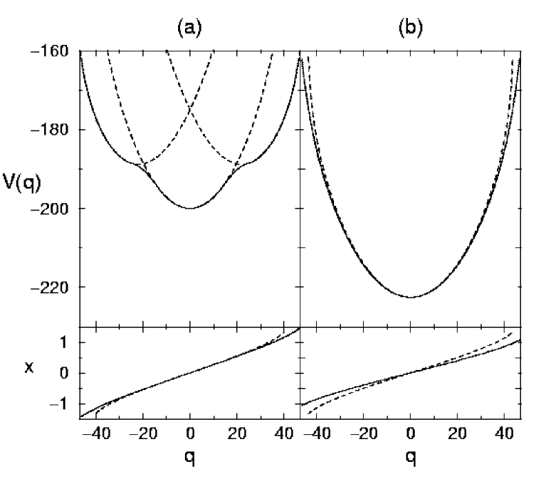
FIG. 45.: The collective potential energy $V(q)$ and the collective coordinate $x$ as a function of the quadrupole moment $q=q_{p}+q_{n}$. We show both the LHA (dashed lines) and the CHB results (solid line) in each figure. The case (a) corresponds to a weak proton pairing force ($G_{p}=0.3$), (b) to a strong pairing force ($G_{p}=10$). The rest of the parameters are given in the main text. The units of all quantities displayed are arbitrary.

As displayed in Fig. 45, the collective potential energy for the weaker pairing strength shows a very interesting behavior, with two shoulders appearing in the CHB collective potential energy. This is what is normally called the adiabatic potential energy, and the shoulders arise from an avoided crossing. As in our previous work [36] the adiabatic LHA method chooses a diabatic (crossing) set of potential energy curves. These shape-coexistence minima are related to 2p-2h excitation in the proton model space, promoting two particles from the lowest Nilsson orbitals to the down-sloping ones. This is of course very similar to the phenomena observed in shape coexistence in semi-magic nuclei.

We get another surprise for the strong pairing case. Here the collective potentials look very similar, and rather structureless, but the collective coordinates are different. This can be traced back to the fact that the collective coordinate in the LHA is not $q_{p}+q_{n}$, but a different combination. At the minimum, the lowest RPA mode correspond approximately to $q_{n}+\frac{1}{10}q_{p}$. This is similar to the situation analyzed in great detail in our study of ²⁸Si, and once again shows the importance of self-consistency in the selection of the collective coordinate. The real collective coordinate is not the mass-quadrupole operator, with consequences that produce discernible differences in the predictions of the two methods.

FIG. 46.: The excitation energies $E_{x}$ and transition matrix elements $|\langle n^{\prime}|Q|n\rangle|$ (numbers next to arrows), in arbitrary units, for the proton-neutron model discussed in the text. The two cases (a) and (b) correspond to those discussed in Fig. 45. In each of the panels the left one (1) is obtained from requantizing the CHB, the middle one (2) is obtained from requantizing the LHA result, and the right one (3) corresponds to the exact diagonalization. Levels denoted by thick lines are doubly degenerate. The numbers next to the arrows denote the size of the transition matrix elements.

In Fig. 46 we show the consequences of these results for the requantization. For the weak pairing case the diabatic picture obtained through the LHA gives almost perfect results, whereas the CHB potential energy curve fails to provide the correct answer. In the case of the strong pairing the incorrect choice of the collective coordinate leads to too large a level spacing in the CHB calculations, whereas the LHA and exact calculations agree again.

For the weak pairing case the exact calculation almost exhibits the doublet structure found from the diabatic potential energy curves; the splitting is less than one part in $10^{5}$ in the exact calculation. Nevertheless, the exact calculation consists of symmetric and antisymmetric states, which leads to the transition matrix element 22.3 between these two states. Since in the LHA calculation the states do not mix, we have printed the diagonal matrix element instead. For very weak mixing this is the correct comparison, as is borne out by the results.

The decoupling measure $D$, Eq. (327), is small for all these cases. The worst case is the strong pairing case, where it rises from $0$ for $q=0$ to $3\times 10^{-3}$ for $q=40$. For this reason we also believe that the “scalar Berry potential” [36] will be small, and we have not included this, or any other quantum corrections, in our calculations.

G Concluding remarks

We have shown that the LHA and/or the GVA give workable tools in situations that might be considered as a guide towards realistic nuclear physics problems.

In the area of shape coexistence, as studied by the model calculations discussed in the last section, and a bit less so for ²⁸Si, it appears that our approaches contain excellent methods to obtain sensible results, with reasonable effort. The problems with the LHA is that even though the size of the space is much smaller than that which enters into a straightforward diagonalization, the application of the local RPA, which needs to be repeated many times at every point along the collective path, may be prohibitive for realistic calculations. Fortunately, many problems can be studied with simplified separable forces, as in the model discussed here. We are at the moment considering the old pairing-plus-quadrupole model, that has been applied so successfully in the physics of heavy nuclei. Such a model can be dealt with much more straightforwardly than more microscopic Skyrme or Gogny-force based approaches. This will allow us to shed light on a good treatment of shape-coexistence, as well on the interesting question of the choice of the collective (cranking) operator, which was already found to be non-trivial in certain limits of the $O(4)$ model.

One might argue that even that is not enough, and we should really adopt a fully microscopic quantum many-body approach. We believe that we can address this problem, and are actively considering the approaches available to us. From the discussion given above, it should be clear that an efficient calculation hinges on efficient solution of the RPA. We are investigating two approaches to this problem, the use of iterative diagonalization of the RPA using Lanczos procedures, or the approximation of the RPA by using separable forces [107], which can be diagonalized much more easily.

In the end such an approach may be more efficient than the path-following version of the GVA, which doesn’t require an RPA diagonalization, but rather depends on a matrix inversion of similar dimensionality, which makes such calculations also very time consuming.

V Quantum theory of LACM and Berry phase

A The Born-Oppenheimer approximation

1 Introduction

Having completed our account of the applications to nuclear physics carried out to date, we turn next to work that is concerned with the further development of the theory. Thus far we have studied large amplitude collective motion on a classical basis and then quantized the emergent collective Hamiltonian. We also developed and applied a theory for computing further corrections arising from the quantum oscillations of the non-collective degrees of freedom. The combined theoretical structure, applied in Secs. IV D and IV E may well suffice for most applications. Nevertheless, in this section we return to the fundamentals of the theory of large amplitude collective motion by seeking to establish a quantum theory from the beginning. We attempted such an approach in our earliest efforts in this field [9, 10], but met with only limited success.

The renewed effort, which we now report, has been rendered more satisfactory by an adaptation of the fundamental notions of the Born-Oppenheimer approximation, including the improvements brought about by the inclusion of the contributions associated with the Berry phase [108, 109]. In this subsection, we deal with the problem without Fermi-Dirac statistics, an account drawn from Ref. [31]. In subsection V B, we present some applications, and in subsection V C, we develop the theory including Fermi-Dirac statistics.

2 Summary of previous viewpoint and its limitations

In contrast to the previous sections, we base our study on a quantum Hamiltonian, that with the help of the summation convention, takes the form

$$H={H}(\xi^{\alpha},\pi_{\alpha})=\frac{1}{8}\{\pi_{\alpha},\{\pi_{\beta},{B}^{\alpha\beta}(\xi)\}\}+{V}(\xi)={T}+{V},$$ (401)

that describes $N$ coordinate and momentum pairs, $\xi^{\alpha}$ and $\pi_{\alpha}$, $\alpha=1,...,N$, which satisfy the canonical commutation relations, using units where $\hbar=1$,

$$[\xi^{\alpha},\pi_{\beta}]=i\delta^{\alpha}_{\beta}.$$ (402)

Associated with this Hamiltonian is a form for the scalar product in Hilbert space that we describe at the end of the current discussion.

Within the quantum mechanical framework, we limit ourselves to locally invertible point transformations,

$$\xi^{\alpha} = g^{\alpha}(q),\;\;q^{\mu}=f^{\mu}(\xi),$$ (403)

$$q = \{Q^{i},q^{a}\},\;\;i=1...K,\;\;a=K+1...N.$$ (404)

For a more concise notation we denote the set of collective coordinates by $Q$, and use $q$ for the non-collective ones. We can now find the Hamiltonian for the new variables. For the potential energy, we have

$${V}(\xi)={V}(g^{\alpha}(Q,q))\equiv\bar{V}(Q,q).$$ (405)

We transform the kinetic energy recognizing the tensor character of the mass matrix and with the help of the relation

$$\pi_{\alpha} = \frac{1}{2}\{f^{\mu}_{,\alpha},p_{\mu}\}.$$ (406)

The justification for (406) is also discussed below. In terms of the new variables, the kinetic energy takes the form

$$T=\frac{1}{8}\{p_{\mu},\{p_{\nu},\bar{B}^{\mu\nu}(Q,q)\}\}+\bar{V}_{\mathrm{quant}}(Q,q),$$ (407)

where the second term, which is specifically a quantum potential arising from the non-commutativity of coordinates and momenta, has the form

$$8\bar{V}_{\mathrm{quant}}(Q,q)=[f^{\mu}_{,\alpha\gamma}g^{\gamma}_{,\nu}g^{\alpha}_{,\lambda}\bar{B}^{\nu\lambda}]_{,\mu}-[f^{\mu}_{,\alpha\gamma}g^{\gamma}_{,\mu}]_{,\nu}g^{\alpha}_{,\lambda}\bar{B}^{\nu\lambda}.$$ (408)

For further work, the momenta are also divided into collective and non-collective subsets, $p_{\mu}=\{P_{i},p_{a}\}$. In order to understand how to decompose the Hamiltonian into collective and non-collective parts on the quantum level, we turn in the next section to a discussion of the Born-Oppenheimer approximation.

 

We define a scalar product and provide the proof of Eq. (406), which specifies how the momentum operator transforms under a general point transformation. It is essential to recognize that this result is tied to a choice of scalar product. We suppose that the Hamiltonian (401) is to be used in conjunction with the metric

$$\langle\Psi_{a}|\Psi_{b}\rangle\equiv\int d\xi^{1}\cdots d\xi^{N}\Psi^{\ast}_{a}(\xi)\Psi_{b}(\xi).$$ (409)

Thus

$$\pi_{\alpha}\rightarrow-i(\partial/\partial\xi^{\alpha}).$$ (410)

Now carry out the point transformation (404) with Jacobian $J$,

$$J=|\partial\xi^{\alpha}/\partial x^{\beta}|.$$ (411)

If we introduce a new wave function

$$\psi_{a}=J^{\frac{1}{2}}\Psi_{a},$$ (412)

the metric is preserved in the sense

$$(\Psi_{a},\Psi_{b})=(\psi_{a},\psi_{b})=\int dx^{1}\cdots dx^{N}\psi^{\ast}_{a}(x)\psi_{b}(x).$$ (413)

This is the metric that is associated with Eq. (406). The proof is given in appendix A of Ref. [31].

 

3 Application of the Born-Oppenheimer approximation

We set ourselves two tasks. We shall first find the leading corrections to the form of the collective Hamiltonian given above, arising from the coupling of the fast to the slow variables. This will be done with the help of the standard Born-Oppenheimer (BO) approximation. In order to evaluate these corrections explicitly, however, we shall then commit ourselves to further approximations for the dependence of the full Hamiltonian on the fast variables, that yield a normal mode description of the latter.

To go beyond the restricted picture presented in Sec. V A 2, we introduce the BO picture into the theory of large amplitude collective motion. To carry this out, we adopt a representation of the wave functions of the collective states $|n\rangle$ in the coordinate space $|Q^{i},q_{a}\rangle\equiv|Q,q\rangle$, of the form

$$\langle Q^{i}q^{a}|n\rangle \equiv \langle Q,q|n\rangle=\sum_{\nu}(Q|n\nu)[q|\nu\!:\!Q],$$ (414)

Here $\nu$ are quantum numbers that describe the state of excitation of the intrinsic degrees of freedom, so that the sum in (414) is over various collective bands, each term representing a product of a wave function for the collective motion and a wave function for the intrinsic motion, the latter tied to the instantaneous value of the collective coordinates. This is the essence of the BO picture, though it is not an approximation until we restrict the sum. We utilize a notation where a ket with an angular bracket indicates a state in the full Hilbert space, a square bracket denotes a state in the space of fast variables (which depends parametrically on the slow variables, as indicated by the notation“$:\!Q$” in the state vector), and a ket with a parenthesis is part of the collective space. We suppose that for fixed $Q$, the states $[q|\nu\!:\!Q]$ are a complete set of functions for the fast coordinates,

$$\sum_{\nu}[q|\nu\!:\!Q][\nu\!:\!Q|q^{\prime}]=\delta(q-q^{\prime}).$$ (415)

Though for the moment we have not specified the equation of which they are the solutions, we shall be able to do so, at least approximately, as a consequence of the developments to be carried out in this section.

For the remainder of the current discussion, we shall consider the simplest case in which the fast variables occupy, for any given value of the slow variables, the state of lowest energy, which is assumed to be non-degenerate. For the case to be studied here, $\nu$ thus takes a single value chosen to be zero. We suppress this zero in the coefficient function that appears in (414), and is now written as $(Q|n)$. This can be identified as the wave function for the collective motion. This identification agrees with the one that was made in the previous sections, where the description of large amplitude collective motion was not tied to a BO approximation. There we emphasized the connection between the decoupled Hilbert space of the collective coordinates and the crucial existence of a $K$-dimensional decoupled coordinate manifold described by the functions $g^{\alpha}(Q,q=0)$. The approximate separability of the associated Hilbert space is based on the assumption that the functions $[q|\nu\!:\!Q]$ describing the fast variables are confined to a narrow region in $q$ space in the neighborhood of the collective surface. If this picture holds, we may expect the mathematical details to work out reasonably.

Adopting the BO approximation, we set ourselves the task of finding an effective Hamiltonian to describe the motion of the collective variables. This operator is defined, though not yet operationally, by means of the equation,

$$(n^{\prime}|H_{{\rm eff}}(Q,P)|n)=\langle n^{\prime}|H(\xi,\pi)|n\rangle.$$ (416)

This relation will assume the status of a definition of the collective Hamiltonian within the space of slow variables and $H_{{\rm eff}}$ recognized as a generalization of $H_{C}$ only after we specify how to eliminate the fast variables from the right hand side. The procedure that we shall follow is closely akin to the traditional BO approach, with characteristic differences arising from the facts that at the beginning we cannot specify which are the slow and which the fast variables, and that the treatment of the fast variables comes as a kind of afterthought, dependent in detail on the prior treatment of the collective variables.

Let us start with the potential energy,

$${V}(\xi)={V}(g^{\alpha}(Q,q))\equiv\bar{V}(Q,q),$$ (417)

and evaluate the associated piece of (416)

$$\langle n^{\prime}|{V}(\xi)|n\rangle \equiv (n^{\prime}|\bar{V}_{{\rm eff}}|n)$$ (418)

$$\cong \int dQdq\,(n^{\prime}|Q)[0\!:\!Q|q]{V}(g^{\alpha}(Q,q))[q|0\!:\!Q](Q|n),$$ (419)

in the BO approximation. Within this framework, the only feasible way of integrating out the fast variables would appear to be to expand $\bar{V}$ in powers of $q^{a}$,

$$\bar{V}(Q,q)=\bar{V}(Q)+\bar{V}_{,a}q^{a}+\frac{1}{2}\bar{V}_{,ab}q^{a}q^{b}+...\;,$$ (420)

leading to

$$\bar{V}_{{\rm eff}}(Q)=\bar{V}(Q)+\bar{V}^{(1)}(Q)+\bar{V}^{(2)}(Q)+...\;,$$ (421)

where, if the function $[q|0\!:\!Q]$ is chosen to be normalized, the various pieces take the form

$$\bar{V}(Q) = \bar{V}(Q,0),$$ (422a)

$$\bar{V}^{(1)}(Q) = \bar{V}_{,a}\int|[q|0\!:\!Q]|^{2}q^{a}\equiv\bar{V}_{,a}(Q)\langle q^{a}\rangle_{Q},$$ (422b)

$$\bar{V}^{(2)}(Q) = \frac{1}{2}\bar{V}_{,ab}(Q)\langle q^{a}q^{b}\rangle_{Q}.$$ (422c)

(In Sec. V C, we shall adopt an alternative method for the nuclear case.)

We thus see that the leading term is independent of the wave function for the fast variables, coinciding with the classical result for the potential energy of large amplitude collective motion. The computation of this term requires only the form of the collective submanifold, $\xi^{\alpha}=g^{\alpha}(Q,0)$, which can be determined by the general theory presented in Sec. II. This is not immediately obvious, since we are dealing with a quantum theory, and the so-called decoupling conditions are operator conditions. These conditions, which follow straightforwardly from decoupling requirements imposed on the transformation (404), are

$$\{p_{i},\bar{B}^{ia}\} = 0,$$ (423)

$$\bar{V}_{,a}+\frac{1}{8}\{p_{i},\{p_{j},\bar{B}^{ij}_{,a}\}\} = 0.$$ (424)

It is apparent that they will be satisfied provided the classical decoupling conditions (33a-33c) are.

To go beyond this lowest order, we need, besides the wave function of the fast variables, to rearrange the expansion of $V$ so that each term in the expansion is a scalar under coordinate transformations. At the conclusion of the present discussion, it is shown that if we wish to interpret the small quantities $q^{a}$ as components of a vector, we must replace the ordinary second derivative by a covariant second derivative, $\bar{V}_{;ab}$, that can be computed from known or calculable quantities according to the equations

$$\bar{V}_{,a}(Q) = {V}_{,\alpha}g^{\alpha}_{,a},$$ (425a)

$$\bar{V}_{;ab}(Q) = {V}_{;\alpha\beta}g^{\alpha}_{,a}g^{\beta}_{,b}.$$ (425b)

Turning now to the quantum corrections, we assume that the decoupling condition, $\bar{V}_{,a}=0$ is sufficiently well satisfied that we can neglect the term $\bar{V}^{(1)}(Q)$. The third term $\bar{V}^{(2)}(Q)$, is the first, $\Delta^{(1)}\bar{V}(Q)$, of a sequence of contributions that we shall identify as the leading corrections to the potential energy.

The remaining terms will arise from the study of the kinetic energy, given after transformation of coordinates by Eqs. (407) and (408). In order to integrate out the fast variables in the contribution that these terms make to $H_{{\rm eff}}$, consider the first term of the kinetic energy. We expand the mass tensor in powers of $q$, and keep initially only the leading term $\bar{B}^{\mu\nu}(Q,0)\equiv\bar{B}^{\mu\nu}(Q)$. In this approximation, we shall first restrict the study to the contribution of those terms where the indices $\mu,\nu$ take on values $i,j$ in the collective subset.

As a preliminary to this calculation, we study the simpler object

$$(n^{\prime}|(P_{i})_{{\rm eff}}|n) = \langle n^{\prime}|P_{i}|n\rangle=(n^{\prime}|(P_{i}-A_{i})|n)\equiv(n^{\prime}|D_{i}|n).$$ (426)

Here $P_{i}$ is the momentum operator in the collective subspace, and

$$A_{i}\equiv i\int dq\,[0\!:\!Q|q]\left(\partial_{Q^{i}}[q|0\!:\!Q]\right).$$ (427)

Notice, however, that if we calculate straightforwardly, the expectation value of $P_{i}P_{j}$ contains an additional contribution,

$$(n^{\prime}|(P_{i}P_{j})_{{\rm eff}}|n) = \langle n^{\prime}|P_{i}P_{j}|n\rangle=(n^{\prime}|(P_{i}P_{j}-A_{i}P_{j}-A_{j}P_{i}+S_{ij})|n),$$ (428)

$$S_{ij} = -\int dq\,[0\!:\!Q|q](\partial_{Q^{i}}\partial_{Q^{j}}[q|0\!:\!Q].$$ (429)

Since $S_{ij}$ is symmetric, it is straightforward to see that the canonical commutation relations among the collective variables projects without change.

It is useful to rewrite (428) in a form that makes contact with standard results. We have as a definition and as a generalization of (427)

$$(i\partial_{j})[q|\nu\!:\!Q] = \sum_{\nu^{\prime}}{}[q|\nu^{\prime}\!:\!Q](A_{j}(Q))_{\nu^{\prime}\nu},$$ (430)

$$(A_{j})_{\nu^{\prime}\nu} = i\int dq\,[\nu^{\prime}\!:\!Q|q]\left(\partial_{Q^{j}}[q|\nu\!:\!Q]\right).$$ (431)

Because of the $Q$ dependence of the matrix element, it now follows that

$$S_{ij} = \sum_{\nu}(A_{i})_{0\nu}(A_{j})_{\nu 0}+(i\partial_{i})A_{j}=(i\partial_{i})A_{j}+A_{i}A_{j}+S^{\prime}_{ij},$$ (432)

$$(A_{j})_{00} = A_{j},\;\;S^{\prime}_{ij}=\sum_{\nu\neq 0}(A_{i})_{0\nu}(A_{j})_{\nu 0}$$ (433)

Consequently, we may also rewrite Eq. (428) as

$$(n^{\prime}|(P_{i}P_{j})_{{\rm eff}}|n)=(n^{\prime}|(D_{i}D_{j}+S^{\prime}_{ij})|n).$$ (434)

In the simplest case, where $[0\!:\!Q|q]$ is a real wave function, it follows that $A_{i}$ vanishes, but the contribution $S^{\prime}_{ij}$ remains to be taken into account.

We are now in a position to apply to the computation of the collective kinetic energy the same reasoning as just carried out for a product of momentum operators. Making use of the analogue of (434), the result is

$$\frac{1}{8}\{D_{i},\{D_{j},B^{ij}(Q)\}\}+\frac{1}{2}S^{\prime}_{ij}B^{ij}.$$ (435)

where the second term can be incorporated into the collective potential energy as a second such contribution, $\Delta^{(2)}\bar{V}(Q)$. An additional contribution of this type is obtained by setting $q^{a}=0$ in Eq. (408),

$$\Delta^{(3)}\bar{V}(Q)=\bar{V}_{\mathrm{quant}}(Q,0),$$ (436)

where $\bar{V}_{\mathrm{quant}}$ is the quantum potential defined in Eqs. (407) and (408).

It remains for us to discuss the contributions from $T$ that depend on $\bar{B}^{ai}(Q)$ that “mix” the collective and non-collective indices and those that depend on the non-collective mass tensor $\bar{B}^{ab}(Q)$. The former can be neglected because of the decoupling condition that the transformed mass tensor does not mix collective and non-collective spaces. The leading contribution of the latter is seen to be another contribution to the potential energy,

$$\Delta^{(4)}\bar{V}=\frac{1}{2}\bar{B}^{ab}(Q)\langle p_{a}p_{b}\rangle_{Q},$$ (437)

where the average is that defined in Eq. (422c).

To summarize our findings, we have derived the following effective Hamiltonian,

$$H_{{\rm eff}}=\frac{1}{8}\{D_{i},\{D_{j},\bar{B}^{ij}(Q)\}\}+\bar{V}(Q)+\Delta\bar{V}(Q),$$ (438)

where $\Delta\bar{V}(Q)$ is the sum of four terms that summarize the leading quantum corrections including the coupling to the fast variables,

$$\Delta\bar{V}=\sum_{i=1}^{4}\Delta^{(i)}\bar{V},$$ (439)

given respectively in or in relation to Eqs. (422c), (435), (436), and (437).

Let us contrast this result with the corresponding form appropriate to the more familiar adiabatic treatment of the structure of molecules. The introduction of a curved metric aside, the main difference is that in the molecular case, the ground state wave function of the fast variables, for a fixed value of $Q$, may be assumed known, and its eigenvalue, $\epsilon_{0}(Q)$, together with $\Delta^{(2)}\bar{V}$, contained in Eq. (435) constitutes the collective potential energy [108, 109]. In the present instance we cannot assume that we know the Hamiltonian of the fast variables, except in an approximate sense that we now discuss. Instead of specializing the transformed Hamiltonian operator to the values $q^{a}=p_{a}=0$, as in the classical limit, we now retain terms up to second order in these variables. In this treatment, we may replace $\bar{V}_{\mathrm{quant}}(Q,q)$ by $\bar{V}_{\mathrm{quant}}(Q,0)$, since this term is already a small correction, and the remaining terms linear in the fast variables may be dropped because of the decoupling conditions. To the specified accuracy, we obtain the following approximate quantum Hamiltonian for the full space,

$$H = H_{\mathrm{C}}+\bar{V}_{\mathrm{quant}}(Q)+H_{\mathrm{NC}},$$ (440a)

$$H_{\mathrm{C}} = \frac{1}{8}\{P_{i},\{P_{j},\bar{B}^{ij}(Q,0)\}\}+\bar{V}(Q,0),$$ (440b)

$$H_{\mathrm{NC}} = \frac{1}{2}p_{a}p_{b}\bar{B}^{ab}(Q)+\frac{1}{2}q^{a}q^{b}\bar{V}_{ab}(Q).$$ (440c)

The justification for this form is that upon application of the BO procedure, it results in the $H_{{\rm eff}}$ that has been derived.

For each value of $Q$, the Hamiltonian $H_{\mathrm{NC}}$ represents a standard normal mode problem. Let $c_{\alpha},c^{{\dagger}}_{\alpha}$ be normal mode destruction and creation operators, $\Omega_{\alpha}$ the corresponding frequencies, and $\hat{n}_{\alpha}=c^{{\dagger}}_{\alpha}c_{\alpha}$. Assuming local stability, i.e., $\Omega_{\alpha}$ real and positive, we have

$$H_{\mathrm{NC}}(Q)=\sum_{\alpha}\left(\hat{n}_{\alpha}(Q)+\mbox{$\frac{1}{2}$}\right)\Omega_{\alpha}(Q).$$ (441)

The practical importance of the contribution of (441) has already been noted in the applications described in Secs. III B and III C, especially the latter, and also in Sec. IV D 6.

The quantum Hamiltonian, expressed in terms of the optimum choice of variables, but in a restricted approximation, has thus been found. Except for the term $\bar{V}_{\mathrm{quant}}(Q)$, it has been expressed in terms of elements that can be readily calculated within the GVA or local RPA. Evaluation of $\bar{V}_{\mathrm{quant}}(Q)$ requires calculation of the curvature of the basic vectors (quantities such as $f^{\mu}_{,\alpha\beta}$). For good decoupling, this term should be small and will be omitted from further consideration.

We return to a discussion of the correction terms, $\Delta\bar{V}$ by which $H_{{\rm eff}}$, Eq. (438), differs from $H_{\mathrm{C}}$. We have just discarded $\Delta^{(3)}\bar{V}$. The sum $\Delta^{(1)}\bar{V}+\Delta^{(4)}\bar{V}$ has been seen in (441) to be a sum of oscillator terms in the approximation considered, its contribution then depending, naturally, on the state of motion of the fast variables. In this section we have considered only the lowest energy state for these variables, so that the contribution of this term is just the zero-point energy.

It remains for us to discuss the contribution of the term $\Delta^{(2)}\bar{V}$, the Berry scalar potential, associated with the projection of the kinetic energy onto the collective subspace. This contribution goes together with that from the “vector potential”, $A_{i}$. The manner in which both the vector and scalar potentials contribute is best studied within the context of the examples worked out in Sec. V C that follows.

 

In terms of the original coordinates, let us consider the change in the potential energy between two neighboring points, $\xi$ and $\xi+\delta\xi$. To second order in $\delta\xi$ we have the usual terms of a Taylor expansion,

$$\Delta V = V(\xi+\delta\xi)-V(\xi)$$ (442)

$$= V_{,\alpha}\delta\xi^{\alpha}+\frac{1}{2}V_{,\alpha\beta}\delta\xi^{\alpha}\delta\xi^{\beta},$$ (443)

that now appears most unsatisfactory, since $\Delta V$ is a scalar, but the second term of (443) contains the ordinary rather than the covariant second derivative. This defect is removed by replacing the quantity $\delta\xi^{\alpha}$ by substitution from the relation

$$d\xi^{\alpha}=\delta\xi^{\alpha}+\frac{1}{2}\Gamma^{\alpha}_{\beta\gamma}\delta\xi^{\beta}\delta\xi^{\gamma},$$ (444)

that contains the Christoffel symbol,

$$\Gamma^{\alpha}_{\beta\gamma}=\frac{1}{2}{B}^{\alpha\delta}({B}_{\delta\beta,\gamma}+{B}_{\delta\gamma,\beta}-{B}_{\beta\gamma,\delta}).$$ (445)

We thus obtain the form

$$\Delta\bar{V}=V_{,\alpha}d\xi^{\alpha}+\frac{1}{2}V_{;\alpha\beta}d\xi^{\alpha}d\xi^{\beta},$$ (446)

where the second term contains the covariant derivative

$$V_{;\alpha\beta}=V_{,\alpha\beta}-\Gamma^{\delta}_{\alpha\beta}V_{,\delta}.$$ (447)

It is now apparent from (446) that $d\xi^{\alpha}$ are the components of a vector, and therefore transformation to any alternative set of coordinates such as the $q^{\mu}$ is standard.

This allows us to calculate the quantity $\bar{V}^{(2)}$ of Eq. (422c) from given dynamical quantities, provided we can define a complete set of coordinate axes at each point of the decoupled manifold. This is done in two stages. In the first stage, the basis vectors at each point of the tangent space to the collective submanifold, for example the set $f^{i}_{\alpha}$, are determined by the algorithm that discovers the collective submanifold. A set of basis vectors $f^{a}_{\alpha}$, orthogonal to the tangent space is then determined (non-uniquely) by the requirement that these be orthogonal to the $f^{i}_{\alpha}$ and to each other with respect to the metric $\tilde{B}^{\alpha\beta}$. The basis vectors orthogonal to the tangent space are precisely the elements needed to compute the Hamiltonian of the fast variables.

 

B Examples with Berry phase

In this subsection we shall discuss a few applications of our formalism. First we shall show the role of the Berry phase in a model where we have degenerate excited states in the non-collective subspace. In the next subsection we shall extend the model to one where the ground state is influenced by the Berry potentials. We shall compare the spectrum of the collective Hamiltonian with that of an exact diagonalization.

Another application of interest is based on a model of Letourneux and Vinet [110, 111] that contains two interacting modes, one representing the low energy quadrupole mode and the other the higher energy dipole mode. We have carried through our own discussion of this model in Ref. [35] but have chosen not to include it in this review.

1 Model with Berry phase in excited states

It is simplest to illustrate the main points by choosing models in which the collective coordinates have already been identified, so that we need not enter into the intricacies of the theory of large amplitude collective motion per se. For instance, in the first model studied below, there are no terms in the Hamiltonian linear in the fast variables. Thus the model satisfies the decoupling conditions exactly. The models worked out in this section come from Ref. [31]. We study the Hamiltonian

$$H = H_{{\rm core}}+H_{{\rm sp}}+H_{{\rm int}}=H_{{\rm core}}+H_{{\rm NC}}$$ (448a)

$$H_{{\rm core}} = \frac{{\mathbf{P}}^{2}}{2M}+V(Q),$$ (448b)

$$H_{{\rm sp}} = \omega(Q)(a_{1}^{{\dagger}}a_{1}+a_{2}^{{\dagger}}a_{2}+1),$$ (448c)

$$H_{{\rm int}} = -G(Q_{-}\,a_{1}^{{\dagger}}a_{2}+Q_{+}\,a_{2}^{{\dagger}}a_{1}).$$ (448d)

Here the coordinates ${\mathbf{Q}}$ and the canonical momenta ${\mathbf{P}}$ are both two-dimensional vectors. We use the notation ${\mathbf{Q}}=(Q_{1},Q_{2})$, $Q_{\pm}=Q_{1}\pm iQ_{2}$, and $Q=(Q_{1}^{2}+Q_{2}^{2})^{1/2}$. (In this section, we are not maintaining the distinction between upper and lower indices.) Furthermore, the $a_{i},a_{i}^{{\dagger}},i=1,2$ are boson destruction and creation operators, $G$ is a coupling strength, and the frequency, $\omega(Q)$, of the uncoupled boson modes has been given a so far unspecified dependence on $Q$ that will be chosen for analytic and numerical convenience. Note that the Hamiltonian, (448a) conserves the boson number,

$$N=a_{1}^{{\dagger}}a_{1}+a_{2}^{{\dagger}}a_{2}={\rm constant}.$$ (449)

Since the $N=0$ problem is completely trivial for this model, the first interesting case is $N=1$. Here, the state vectors may be written exactly as a superposition

$$|n\rangle=\int d{\mathbf{Q}}\,\{({\mathbf{Q}}|n1)a_{1}^{{\dagger}}|0]+({\mathbf{Q}}|n2)a_{2}^{{\dagger}}|0]\},$$ (450)

where $|0]$ is the vacuum state. The use of square brackets for the vacuum state of the fast variables is consistent with the notation introduced earlier. The resulting eigenvalue equation in the space of the collective variables, ${\mathbf{Q}}$, is determined by the two-by-two effective Hamiltonian, $H_{\mathrm{eff}}$, with matrix elements

$$(H_{{\rm eff}})_{11} = H_{{\rm core}}+2\omega(Q)=(H_{{\rm eff}})_{22},$$ (451a)

$$(H_{{\rm eff}})_{12} = -GQ_{-}=(H_{{\rm eff}})_{21}^{\ast}.$$ (451b)

Below we shall describe exact solutions of the associated Schrödinger equation.

These exact solutions are to be compared with the adiabatic approximation, with and without the Berry potential terms. For this approximation, we require the normal modes of $H_{\mathrm{NC}}$, which we calculate in a standard way from the equations of motion,

$$[a_{1},H_{\mathrm{NC}}] = \omega a_{1}-GQ_{-}a_{2},$$ (452)

$${}[a_{2},H_{\mathrm{NC}}] = \omega a_{2}-GQ_{+}a_{1},$$ (453)

by forming the matrix elements,

$$\psi_{i}=[0|a_{i}|\Psi].$$ (454)

With $\Omega$ representing the energy of the state $|\Psi]$, , we obtain the equations

$$\Omega\psi_{1} = \omega\psi_{1}-GQ_{-}\psi_{2},$$ (455)

$$\Omega\psi_{2} = -GQ_{+}\psi_{1}+\omega\psi_{2},$$ (456)

that yield the eigenvalues

$$\Omega^{(1)}(Q) = \omega(Q)-GQ,$$ (457)

$$\Omega^{(2)}(Q) = \omega(Q)+GQ,$$ (458)

that are degenerate when $Q=0$. The associated normalized solutions of (456) are represented most conveniently by introducing the normal-mode creation operators

$$b_{i}^{{\dagger}}=\psi^{(i)}_{j}a_{j}^{{\dagger}}.$$ (459)

We make the explicit choice

$$b_{1}^{{\dagger}} = \frac{1}{\sqrt{2}}a_{1}^{{\dagger}}+\frac{1}{\sqrt{2}}\exp{i\phi({\mathbf{Q}})}a_{2}^{{\dagger}},$$ (460a)

$$b_{2}^{{\dagger}} = \frac{1}{\sqrt{2}}\exp{i\phi({\mathbf{Q}})}a_{1}^{{\dagger}}-\frac{1}{\sqrt{2}}a_{2}^{{\dagger}},$$ (460b)

$$\tan\phi({\mathbf{Q}}) = Q_{2}/Q_{1}.$$ (460c)

We apply these elementary results to the adiabatic approximation. In this case we represent a suitable subset of the eigenfunctions (450) in the form

$$|n\rangle=\int d{\mathbf{Q}}\,({\mathbf{Q}}|n)b_{1}^{{\dagger}}|0\!:\!Q],$$ (461)

where the notation $|0\!:\!Q]$ refers to the vacuum for the normal modes. (For the current model, it coincides with the uncoupled vacuum.) The considerations of Sec. V A 3 now apply to this class of state vectors and, in particular, we apply Eq. (434). As a special case of this equation, we have

$$\sum_{i}(P_{i})^{2} \rightarrow \sum_{i}(P_{i}-A_{i})^{2}+\sum_{i}|(A_{i})_{21}|^{2},$$ (462)

$$A_{i} = i[0\!:\!Q|b_{1}\partial_{i}b_{1}^{{\dagger}}|0\!:\!Q],$$ (463a)

$$(A_{i})_{21} = i[0\!:\!Q|b_{2}\partial_{i}b_{1}^{{\dagger}}|0\!:\!Q],$$ (463b)

With the help of Eqs. (460a) and (460b), the quantities of interest are found to take the values

$${\mathbf{A}} = \frac{1}{2Q^{2}}(Q_{2},-Q_{1}),$$ (464)

$$\sum_{i}|(A_{i})_{21}|^{2} = (1/4Q^{2}).$$ (465)

As expected these results are singular for $Q=0$, which is where the two states become degenerate and the adiabatic approximation breaks down. The collective or adiabatic Hamiltonian, $H_{\mathrm{C}}$, that thus emerges from the assumption that the state vectors of interest can be written in the form (461), has the structure

$$H_{\mathrm{C}}=(1/2M)[({\mathbf{P}}-{\mathbf{A}})^{2}+({\mathbf{A}}_{21})^{2}]+{V}(Q)+(3/2)\Omega^{(1)}(Q)+(1/2)\Omega^{(2)}(Q).$$ (466)

We turn to the problem of solving the associated eigenvalue problem. We wish to compare the results of exact (numerical) calculations with the eigenvalues of the collective Hamiltonian. It is useful to choose $\omega(Q)$ such that the latter is exactly solvable. One such choice is

$$\omega(Q)=\frac{1}{2}GQ.$$ (467)

In this case the additional contribution to the potential is zero,

$$\frac{3}{2}\Omega^{(1)}(Q)+\frac{1}{2}\Omega^{(2)}(Q)=0.$$ (468)

We further take $M=1$ and $V(Q)=\frac{1}{2}Q^{2}$. We use the definition of the two-dimensional angular momentum,

$$L = -i\frac{\partial}{\partial\phi}=-i(Q_{1}P_{2}-Q_{2}P_{1}),$$ (469)

to simplify the ${{\mathbf{P}}}\cdot{{\mathbf{A}}}$ term. We can further simplify the equation $H_{c}\psi({\mathbf{Q}})=E\psi({\mathbf{Q}})$ by substituting

$$\psi({\mathbf{Q}})=Q^{-1/2}\chi(Q){\rm e}^{im\phi}$$ (470)

and find

$$\left\{-\frac{1}{2}\frac{d^{2}}{dQ^{2}}+\frac{1}{2Q^{2}}\left[m^{2}+m+\frac{1}{4}\right]+\frac{1}{2}Q^{2}\right\}\chi(Q)=E\chi(Q).$$ (471)

Even though the centrifugal term is different, this is still very similar to the radial equation for the two-dimensional harmonic oscillator. It can be solved by the substitution

$$\chi(q)=q^{\alpha+1/2}{\rm e}^{-q^{2}/2}L_{n}^{(\alpha)}(q^{2}),$$ (472)

As is well known, the Laguerre function $L_{n}^{(\alpha)}$ satisfies the equation

$$-\frac{d^{2}}{dq^{2}}L_{n}^{(\alpha)}+(q^{2}+\frac{1-4\alpha^{2}}{4q^{2}})L_{n}^{(\alpha)}=(4n+2\alpha+2)L_{n}^{(\alpha)}.$$ (473)

We thus find that

$$\alpha(m) = \sqrt{1/4+(m+1/2)^{2}},$$ (474)

$$E_{nm} = (2n+\alpha(m)+1).$$ (475)

Without the Berry’s phase terms we would have found

$$E_{nm}=(2n+|m|+1).$$ (476)

When $G=0$ the solution (476) is exact. Thus Eq. (475), which is independent of $G$, cannot be valid for all $G$. It should be valid in the adiabatic limit, which means that the two frequencies $\Omega$ must be very different. This occurs when $G$ is very large.

The exact solution of the problem can be calculated using a harmonic oscillator basis in circular coordinates for the $Q$ degrees of freedom. This is coupled to a state containing either one $a^{\dagger}_{1}$ or one $a^{\dagger}_{2}$ boson,

$$|n,m,n_{1},n_{2}\rangle=|n,m)(a^{\dagger}_{1})^{(n_{1})}(a^{\dagger}_{2})^{(n_{2})}|0],\;\;n_{1}+n_{2}=1.$$ (477)

The interaction Hamiltonian only couples states with $n_{1}=1,m=m_{1}$ to states with $n_{2}=1,m=m_{1}+1$, but also changes the radial quantum number of the oscillator. We can thus choose the value of $m_{1}$. Since we wish to obtain accurate results for large $G$, we allow the number of $Q$ harmonic oscillator quanta to be fairly large. We have used up to 200 harmonic oscillator states in each block (which leads to a 400 by 400 matrix eigenvalue problem).

In Table VII we give a selected set of results for $m_{1}=0$ and a number of values of $G$. Similar results for $m_{1}=1$ are listed in Table VIII. We clearly see the convergence to the collective model results including the Berry phase for large $G$.

TABLE VII.: The lowest 10 eigenvalues of the coupled problem for $m_{1}=0$ as a function of $G$. The column labeled Berry lists the eigenenergies of the collective Hamiltonian (466).

G	0.01	0.1	1	10	100	1000	Berry
$E_{1}$	1.00875	1.07849	1.36229	1.58463	1.66532	1.69302	1.7071
$E_{2}$	2.01328	2.13134	2.92007	3.48844	3.63505	3.68298	3.7071
$E_{3}$	3.01540	3.14492	4.09426	5.39473	5.60870	5.67438	5.7071
$E_{4}$	4.01827	4.18125	5.30157	7.29413	7.58443	7.66658	7.7071
$E_{5}$	5.01997	5.19061	6.57000	9.17666	9.56145	9.65932	9.7071
$E_{6}$	6.02221	6.22068	7.66964	11.0262	11.5393	11.6525	11.7071
$E_{7}$	7.02367	7.22768	8.90918	12.8133	13.5177	13.6459	13.7071
$E_{8}$	8.02558	8.25425	10.0230	14.4981	15.4965	15.6396	15.7071
$E_{9}$	9.02687	9.25972	11.1883	16.0926	17.4754	17.6335	17.7071
$E_{10}$	10.0286	10.2840	12.3410	17.7119	19.4544	19.6276	19.7071

TABLE VIII.: The lowest 10 eigenvalues of the coupled problem for $m_{1}=1$ as a function of $G$. The column labeled Berry lists the eigenenergies of the collective Hamiltonian (466).

G	0.01	0.1	1	10	100	1000	Berry
$E_{1}$	2.01308	2.11333	2.41566	2.54921	2.57601	2.58042	2.58114
$E_{2}$	3.01670	3.17369	4.20360	4.51926	4.57057	4.57959	4.58114
$E_{3}$	4.01807	4.16340	5.44213	6.48766	6.56479	6.57866	6.58114
$E_{4}$	5.02086	5.21512	6.43129	8.45380	8.55880	8.57766	8.58114
$E_{5}$	6.02202	6.20307	7.86356	10.4165	10.5527	10.5766	10.58114
$E_{6}$	7.02436	7.25000	8.79958	12.3739	12.5464	12.5755	12.58114
$E_{7}$	8.02538	8.23691	10.1070	14.3218	14.5400	14.5744	14.58114
$E_{8}$	9.02745	9.28063	11.1975	16.2512	16.5336	16.5733	16.58114
$E_{9}$	10.0284	10.2669	12.3141	18.1346	18.5270	18.5721	18.58114
$E_{10}$	11.0302	11.3082	13.5364	19.8627	20.5204	20.5709	20.58114

2 Model with ground-state correlations

We next study a model differing from the one just investigated only in the form of the interaction. In this model Eqs. (448a)-(448c) stand as given, but Eq. (448d) is modified to [31]

$$H_{{\rm int}} = -G_{0}Q(a_{1}^{{\dagger}}a_{2}+a_{2}^{{\dagger}}a_{1})-G_{1}(Q_{+}a_{1}a_{2}+Q_{-}a_{1}^{{\dagger}}a_{2}^{{\dagger}}).$$ (478)

The second term of this interaction spoils the conservation of boson number used to simplify the solution of the previous problem. For the present problem, it is already interesting to study the spectrum when the fast variables are in their ground levels, since there are now non-trivial ground-state correlations and associated non-trivial Berry potentials, that we shall calculate.

We first turn to the study of the BO approximation. As before we need the normal modes of the fast variables, as determined from the equations of motion

$$[a_{1},H_{\mathrm{NC}}] = \omega a_{1}-G_{0}Qa_{2}-G_{1}Q_{-}a_{2}^{{\dagger}},$$ (479)

$${}[a_{2},H_{\mathrm{NC}}] = \omega a_{2}-G_{0}Qa_{1}-G_{1}Q_{-}a_{1}^{{\dagger}},$$ (480)

and their hermitian conjugates. In terms of the definitions

$$b_{i}^{{\dagger}} = \psi_{j}^{(i)}a_{j}^{{\dagger}}-\chi_{j}^{(i)}a_{j},$$ (481)

$$\psi_{j}^{(i)} = [0\!:\!Q|a_{j}|\Psi^{(i)}],$$ (482)

$$\chi_{j}^{(i)} = [0\!:\!Q|a_{j}^{{\dagger}}|\Psi^{(i)}],$$ (483)

$$|\Psi^{(i)}] = b_{i}^{{\dagger}}|0\!:\!Q],$$ (484)

we obtain the eigenvalue equations

$$\Omega\psi_{1} = \omega\psi_{1}-G_{0}Q\psi_{2}-G_{1}Q_{-}\chi_{2},$$ (485)

$$\Omega\psi_{2} = \omega\psi_{2}-G_{0}Q\psi_{1}-G_{1}Q_{-}\chi_{1},$$ (486)

$$-\Omega\chi_{1} = \omega\chi_{1}-G_{0}Q\chi_{2}-G_{1}Q_{+}\psi_{1},$$ (487)

$$-\Omega\chi_{2} = \omega\chi_{2}-G_{0}Q\chi_{1}-G_{1}Q_{+}\psi_{1}.$$ (488)

The physical eigenvalues are the positive roots of

$$\Omega^{2}(Q)=(\omega\mp G_{0}Q)^{2}-G_{1}^{2}Q^{2},$$ (489)

which are again degenerate at $Q=0$. As for the first model studied, we label these solutions $\Omega^{(i)},i=1,2$. The corresponding amplitudes are determined from the equations of motion and the normalization conditions

$$|\psi_{1}|^{2}+|\psi_{2}|^{2}-|\chi_{1}|^{2}-|\chi_{2}|^{2}=1.$$ (490)

The simplest forms for the amplitudes are achieved by repeated use of the eigenvalue condition (489). We thus find

$$\psi_{2}^{(j)} = (-1)^{j+1}\psi_{1}^{(j)}={\rm real},$$ (491)

$$\chi_{i}^{(j)} = \exp(i\phi)\tilde{\chi}_{i}^{(j)},$$ (492)

$$\tilde{\chi}_{2}^{(j)} = (-1)^{j+1}\tilde{\chi}_{1}^{(j)}={\rm real},$$ (493)

$$\psi_{1}^{(j)} = \frac{(\Omega^{(j)}+\omega)+(-1)^{j}G_{0}Q}{\sqrt{2}[(\omega+\Omega^{(j)})^{2}+(-1)^{j}2G_{0}Q(\omega+\Omega^{(j)})+(G_{0}^{2}-G_{1}^{2})Q^{2}]^{1/2}},$$ (494)

$$\chi_{1}^{(j)} = (-1)^{j+1}f^{(j)}(Q)\psi_{1}^{(j)},$$ (495)

$$f^{(j)} = \frac{G_{1}Q}{(\Omega^{(j)}+\omega)+(-1)^{j}G_{0}Q}.$$ (496)

Here $\phi$ is the polar angle for $Q$, $\phi={\rm arctan}(Q_{2}/Q_{1})$.

These results are thus available for application to the BO approximation studied by means of the assumption

$$|n\rangle=\int d{\mathbf{Q}}\,|{\mathbf{Q}})({\mathbf{Q}}|n)|0\!:\!Q].$$ (497)

It follows that the Berry vector potential is given by the formula

$$A_{i}=i[0\!:\!Q|\partial_{i}|0\!:\!Q].$$ (498)

To carry out this calculation, we need the form of the correlated vacuum state, as given by the equation, see Ref. [112],

$$|0\!:\!Q]={\cal N}\exp[\frac{1}{2}Z_{ij}a_{i}^{{\dagger}}a_{j}^{{\dagger}}]|0],$$ (499)

where ${\cal N}$ is a real normalization factor, whose value we shall not need, $a_{i}|0]=0$, and $Z_{ij}$ is a generally complex array whose role will be considered in more detail below. Using the constancy of the norm of the correlated ground state as a function of the values of ${\mathbf{Q}}$, we can rewrite (498) as

$$A_{i}=\frac{1}{2}i\left\{[0\!:\!Q|\partial_{i}|0\!:\!Q]-[\partial_{i}0\!:\!Q|0\!:\!Q]\right\},$$ (500)

which shows that the derivative of the (real) normalization factor ${\cal N}$ does not contribute. This leaves the result

$$A_{i}=\frac{1}{4}i\left[\langle a_{k}^{{\dagger}}a_{l}^{{\dagger}}\rangle\partial_{i}Z_{kl}-\langle a_{k}a_{l}\rangle\partial_{i}Z_{kl}^{\ast}\right],$$ (501)

where the averages, indicated by angular brackets, are with respect to the correlated vacuum.

We next indicate how (501) can be evaluated in terms of the solutions we have found above for the equations of motion. The quantities $Z_{kl}$ are solutions of the equations

$$\psi_{j}^{(i)}Z_{jk}^{\ast}=\chi_{k}^{(i)},$$ (502)

that follow from the definition $b_{i}|0\!:\!Q]=0.$ The expectation values can also be evaluated with the help of the formulas

$$a_{i}=\psi_{i}^{(j)}b_{j}+\chi_{i}^{(j)\ast}b_{j}^{{\dagger}},$$ (503)

and their hermitian conjugates, that are the inverse to Eq. (481). An elementary calculation now yields

$$\langle a_{k}^{{\dagger}}a_{l}^{{\dagger}}\rangle=\langle a_{k}a_{l}\rangle^{\ast}=\chi_{k}^{(j)}\psi_{l}^{(j)\ast}.$$ (504)

Thus for the vacuum Berry potential, we obtain the formula

$$A_{i}=\frac{1}{4}i\left[\chi_{k}^{(m)}\psi_{l}^{(m)\ast}\partial_{i}Z_{kl}-\chi_{k}^{(m)\ast}\psi_{l}^{(m)}\partial_{i}Z_{kl}^{\ast}\right].$$ (505a)

Any other matrix element, $(A_{i})_{\nu 0}$ of the Berry potential can be calculated by similar techniques. In fact, the only non-vanishing elements of this type are $(A_{i})_{11,0}$, $(A_{i})_{20,0}$, and $(A_{i})_{02,0}$, where, for example, $\nu=20$ means a state with two correlated bosons of type 1 and none of type 2. We quote formulas for these matrix elements that follow from the same elementary techniques that furnished Eq. (505a). We thus have

$$(A_{i})_{11,0} = i[11\!:\!Q|\partial_{i}|0\!:\!Q]=-i[\partial_{i}\;11\!:\!Q|0\!:\!Q]=-i[0\!:\!Q|b_{1}\partial_{i}(b_{2})|0\!:\!Q]\}$$ (505b)

$$= -i\left[\sum_{j}\psi_{j}^{(1)\ast}\partial_{i}\chi_{j}^{(2)\ast}-\chi_{j}^{(1)\ast}\partial_{i}\psi_{j}^{(2)\ast}\right].$$ (505c)

Similarly, remembering the normalization of the states, we find

$$(A_{i})_{20,0}=\frac{1}{i\sqrt{2}}\left[\sum_{j}\psi_{j}^{(1)\ast}\partial_{i}\chi_{j}^{(1)\ast}-\chi_{j}^{(1)\ast}\partial_{i}\psi_{j}^{(1)\ast}\right].$$ (505d)

Finally, the matrix element $(A_{i})_{02,0}$ is obtained from (505d) simply by replacing all superscripts 1 by 2.

In order to implement fully the BO approximation, it is necessary to evaluate these matrix elements in terms of the explicit solutions of the model displayed in Eqs. (496). It is also appropriate to remark here that in consequence of these relations and Eq. (502) we can write

$$Z_{jk}=\exp(-i\phi)\tilde{Z}_{jk},\;\;\tilde{Z}_{jk}={\rm real}$$ (506)

The calculation of the Berry potentials as defined above is now straightforward. In terms of purely real quantities, we find, for example,

$$A_{i}=(\partial_{i}\phi)[(\tilde{\chi}_{1}^{(1)}\psi_{1}^{(1)}+\tilde{\chi}_{1}^{(2)}\psi_{1}^{(2)})\tilde{Z}_{11}+(\tilde{\chi}_{1}^{(1)}\psi_{1}^{(1)}-\tilde{\chi}_{1}^{(2)}\psi_{1}^{(2)})\tilde{Z}_{12}].$$ (507)

Using the real form of Eq. (502), this expression can be simplified to

$${\mathbf{A}} = {\mathbf{\partial}}\phi[(\tilde{\chi}_{1}^{(1)})^{2}+(\tilde{\chi}_{1}^{(2)})^{2}]$$ (508)

$$= \frac{G_{1}^{2}}{2}\left[\frac{1}{(\omega+\Omega^{(1)})(\omega+\Omega^{(1)}-2G_{0}Q)+(G_{0}^{2}-G_{1}^{2})Q^{2}}\right.$$ (510)

$$\left.+\frac{1}{(\omega+\Omega^{(2)})(\omega+\Omega^{(2)}+2G_{0}Q)+(G_{0}^{2}-G_{1}^{2})Q^{2}}\right](-Q_{2},Q_{1})_{i}.$$

In contrast to the previous model the vector potential is not singular at the origin, but take the finite value

$${\mathbf{A}}(0)=\frac{G_{1}^{2}}{4\omega(0)^{2}}(-Q_{2},Q_{1}).$$ (511)

Turning to the off-diagonal matrix elements, we find by similar calculations

$$(A_{i})_{11,0} = 0,$$ (512a)

$$(A_{i})_{20,0} = \sqrt{2}\exp(-i\phi)[(\partial_{i}\phi)\psi_{1}^{(1)}\tilde{\chi}_{1}^{(1)}+i(\psi_{1}^{(1)}\partial_{i}\tilde{\chi}_{1}^{(1)}-\tilde{\chi}_{1}^{(1)}\partial_{i}\psi_{1}^{(1)}]$$ (512b)

$$= -\sqrt{2}\exp(-i\phi)\left(\psi_{1}^{(1)}\right)^{2}f^{(1)}\left[\partial_{i}\phi+i(\partial_{i}Q)\partial_{Q}\ln f^{(1)}\right]$$ (512c)

$$= \sqrt{2}\exp(-i\phi)\frac{G_{1}[(\Omega^{(1)}+\omega)-G_{0}Q]}{2[(\omega+\Omega^{(1)})(\omega+\Omega^{(1)}-2G_{0}Q)+(G_{0}^{2}-G_{1}^{2})Q^{2}]}$$ (512e)

$$\times\left[\frac{1}{Q}(-Q_{2},Q_{1})+i\frac{1}{Q}(Q_{1},Q_{2})Q\partial_{Q}\ln f^{(1)}\right],$$

$$(A_{i})_{02,0} = -\sqrt{2}\exp(-i\phi)\frac{G_{1}[G_{0}Q+(\Omega^{(2)}+\omega)]}{2[(\omega+\Omega^{(2)})(\omega+\Omega^{(2)}-2G_{0}Q)+(G_{0}^{2}-G_{1}^{2})Q^{2}]}$$ (512g)

$$\times\left[\frac{1}{Q}(-Q_{2},Q_{1})+i\frac{1}{Q}(Q_{1},Q_{2})Q\partial_{Q}\ln f^{(2)}\right].$$

These off-diagonal potentials are also regular as $Q$ goes to zero, for reasonably well behaved $\omega(Q)$.

We now study the numerical solution of the adiabatic Hamiltonian,

$$H_{\mathrm{C}}=\frac{1}{2}\left[({\mathbf{P}}-{\mathbf{A}})^{2}+|{\mathbf{A}}_{20,0}|^{2}+|{\mathbf{A}}_{02,0}|^{2}\right]+\frac{1}{2}Q^{2}+\frac{1}{2}\left[\Omega^{(1)}(Q)+\Omega^{(2)}(Q)\right],$$ (513)

where we have once again made the choice $M=1,V(Q)=\frac{1}{2}Q^{2}$. For simplicity we take $G_{0}=0$, and write $G_{1}=G$. For this special choice $\Omega^{(1)}=\Omega^{(2)}=\Omega$ and $(A_{i})_{02,0}=-(A_{i})_{20,0}$. A simple form for $\omega(Q)$, chosen such that $\Omega$ is positive definite, is

$$\omega(Q)=\omega_{0}+GQ.$$ (514)

In Fig. 47 we show some of the relevant quantities in the collective Hamiltonian for the choice $G=1$, $\omega_{0}=2$.

FIG. 47.: Parameters in the collective Hamiltonian for $G=1$, $\omega_{0}=2$. The lower panel shows the frequencies $\Omega^{(j)}$, the middle panel shows the size of the diagonal Berry potential, and the upper panel shows the square of the off-diagonal Berry-potentials.

We diagonalize the collective Hamiltonian by first going to circular coordinates, and obtain a radial equation using angular momentum conservation, which holds obviously by construction for the exact Hamiltonian but is also a property of the BOA. We then map the $Q$ values from the interval $[0,\infty]$ to the interval $[0,1]$. Finally we make a finite difference approximation to the radial equation, and solve the approximate equation by matrix diagonalization.

Solving the complete problem, without making the adiabatic approximation is somewhat involved. Since the Hamiltonian is invariant under the interchange $a^{\dagger}_{1}\leftrightarrow a^{\dagger}_{2}$, we introduce new operators that are invariant under this parity transformation,

$$a^{\dagger}_{\pm}=\frac{1}{\sqrt{2}}(a^{\dagger}_{1}\pm a^{\dagger}_{2}).$$ (515)

The interaction Hamiltonian takes the simple form

$$H_{{\rm int}}=-G_{0}(a^{\dagger}_{+}a_{+}-a^{\dagger}_{-}a_{-})-\frac{G_{1}}{2}(Q_{+}[a_{+}^{2}-a_{-}^{2}]+Q_{-}[a_{+}^{\dagger 2}-a_{-}^{\dagger 2}]).$$ (516)

We now make the expansion

$$\Psi=\sum_{K,\kappa}\psi_{K,\kappa}(Q)\frac{\left(a^{\dagger}_{+}\right)^{2K-2\kappa}\left(a^{\dagger}_{-}\right)^{2\kappa}}{\sqrt{(2K-2\kappa)!(2\kappa)!}}|0]$$ (517)

(The even powers in this equation constitute the only combination that includes the vacuum for the fast degrees of freedom.)

An approximate solution is obtained by limiting the sum over $K$, while summing over all allowed $\kappa$. At the same time we expand $\psi_{K,\kappa}(Q)$ in a finite number of circular harmonic oscillator eigenfunctions $\langle Q|nm\rangle$. We denote the $m$ value used in the expansion of $\psi_{K,\kappa}(Q)$ by $m_{K,\kappa}$. The interaction does not couple states of different $\kappa$ for fixed $K$. We thus find that $m_{K,\kappa}=m_{K}=m_{K-1}-1$. Thus the value $m_{0}$ is a constant of the motion, and can be used to specify different solutions. This quantity corresponds directly to the value of $m$ in the collective Hamiltonian. We have performed matrix diagonalizations for $\omega_{0}=2,10$ and $G=1$, using harmonic oscillator states up to principal quantum number 70, and $K$ values up to 20. (This corresponds to a 61,401 by 61,401 matrix.) The resulting matrix, which is very sparse, was diagonalized using a Lanczos algorithm. The eigenvalues were checked for convergence by comparing a calculation with smaller cut-offs on $n$ and $K$ against one with larger cutoffs. In Tables IX and X we compare a few selected ground state energies of the complete collective Hamiltonian with the exact solution. The splitting between states with opposite values of $m$ is completely due to the vector potential. For the case $\omega_{0}=2$, where the adiabatic approximation is of questionable validity, we see that the size of the splitting is very close to the exact value. The difference is probably due to non-adiabatic effects that can not be completely neglected for $\omega_{0}=2$. For the case $\omega_{0}=10$ the correspondence is much closer, but the size of the Berry vector potential is much smaller as well.

TABLE IX.: A comparison between the exact numerical ground state energies and those for the collective Hamiltonian. $\omega_{0}=2,G=1$, and the values of $m$ are listed in the table.

	$m=-5$	$m=5$	$m=-1$	$m=1$
exact	9.54715	9.73101	4.97309	5.03405
collective	9.56722	9.74656	4.98669	5.04375

TABLE X.: A comparison between the exact numerical ground state energies and those for the collective Hamiltonian. $\omega_{0}=10,G=1$, and the values of $m$ are listed in the table.

	$m=-5$	$m=5$
exact	18.0745	18.0918
collective	18.0750	18.0922

C Born-Oppenheimer approximation and Berry phase: Fermi-Dirac statistics

1 Introduction

In this section, we consider the extension of the ideas presented in Sec. V A 3 to the nuclear case. A short route that suggests itself is to follow the scheme carried out in Sec. IV A which is to transcribe previous results, such as Eqs. (440a) - (440c) to the nuclear case. A major objection to this course (among others) is that the small oscillations Hamiltonian, $H_{\mathrm{NC}}$ of Eq. (440c) will not accurately describe the first quantum corrections to the quantized classical Hamiltonian. This was a principal result (quoted) in Sec. IV D 6. We therefore set for the goal of this section the derivation ab initio of a quantum theory of large amplitude collective, applicable to the nuclear case. We shall again rely on the Born-Oppenheimer approximation (BOA), but a major difference compared with the previous considerations is that we shall not introduce a localized basis for the intrinsic degrees of freedom. The contents of this section represent a major revision of the ideas presented in Refs. [34, 35].

2 Definition of the effective Hamiltonian

We study the problem defined by the shell-model Hamiltonian

$$H=h_{\alpha\beta}a^{{\dagger}}_{\alpha}a_{\beta}+\frac{1}{4}V_{\alpha\beta\gamma\delta}a^{{\dagger}}_{\alpha}a^{{\dagger}}_{\beta}a_{\delta}a_{\gamma},$$ (518)

expressed in terms of the usual fermion creation (destruction) operators, $a^{{\dagger}}_{\alpha}(a_{\alpha})$ describing the shell-model orbit $\alpha$, and in terms of the hermitian one- and two-particle Hermitian matrices $h$ and $V$; the latter, as written, is also antisymmetric, separately, in the initial and in the final pair of indices.

In order to carry out the program we have in view, we assume once more that there exists a basis of states that is a product of localized states for the collective coordinates and “oscillator-like” states for the intrinsic coordinates, each complete in its own subspace

$$|Q^{i},\nu\!:\!Q\rangle = |Q)|\nu\!:\!Q],$$ (519)

$$\sum_{\nu}|\nu\!:\!Q][\nu\!:\!Q| = 1_{\mathrm{NC}},$$ (520)

where $1_{\mathrm{NC}}$ is the unit operator in the non-collective space. In terms of this basis set, which remains to be characterized in more detail, we assume the existence of a Hilbert space of collective states, $|n\rangle$, that can be represented in the general BO form

$$|n\rangle=\sum_{\nu}\int dQ\,|Q)(Q|n\nu)|\nu\!:\!Q].$$ (521)

In contrast to the molecular case, or to specially chosen simple examples, it is generally not possible to specify ahead of time the Hamiltonian of which the $|\nu\!:\!Q]$ are the state vectors. Ultimately, as a consequence of the further development of the theory, we shall be able to obtain an approximate characterization of the space of the fast variables, adequate for most of our needs. In the usual BOA or adiabatic approximation, to which the considerations that follow pertain, we restrict the set $\nu$ in (521) to the ground-state value $0$. Nevertheless, we shall see that the formalism forces the excited intrinsic states back into the picture.

The next step is to derive an effective Hamiltonian for the collective subspace, defined within the BOA by the equation

$$(n|H_{\rm eff}(Q,P)|n^{\prime})\equiv\langle n|H|n^{\prime}\rangle=\int dQdQ^{\prime}(n|Q)[0\!:\!Q|(Q|H|Q^{\prime})|0\!:\!Q^{\prime}](Q^{\prime}|n^{\prime}),$$ (522)

which has utilized the BOA in the form of Eq. (521) with the sum restricted to the single term $\nu=0$. We wish $H_{\rm eff}$ to depend only on the collective variables, $Q$, and their canonically conjugate momenta, $P$. The method is to make a moment expansion of the matrix element $(Q|H|Q^{\prime})$, which is still an operator in the intrinsic space. We define

$$(Q|H|Q^{\prime}) \equiv K(\bar{Q},\tilde{Q}),$$ (523)

$$\bar{Q} = \frac{1}{2}(Q+Q^{\prime}),~{}~{}~{}\tilde{Q}=Q-Q^{\prime}.$$ (524)

With the assumption that the matrix elements (523) are peaked in the differences of collective coordinates, we can carry out an expansion in terms of the delta function and its derivatives with respect to such coordinates,

$$K(\bar{Q},\tilde{Q}) = K^{(0)}(\bar{Q})\delta(\tilde{Q})+K^{(1,i)}(\bar{Q})(-i\tilde{\partial}_{i})\delta(\tilde{Q})$$ (526)

$$+\frac{1}{2}K^{(2,ij)}(\bar{Q})(-i\tilde{\partial}_{i})(-i\tilde{\partial}_{j})\delta(\tilde{Q})+\cdots.$$

In this expression the various coefficient functions are examples of the set of moments

$$K^{(n,i_{1}\cdots i_{n})}(\bar{Q})=\int d\tilde{Q}(-i)^{n}\tilde{Q}^{i_{1}}\cdots\tilde{Q}^{i_{n}}K(\bar{Q},\tilde{Q}).$$ (527)

We expect the moment expansion for the collective variables to generate a convergent series in powers of the reciprocal of the number of particles participating in the collective motion.

Inserting this expansion into Eq. (522), we easily succeed in identifying the operator $H_{\rm eff}(Q,P)$. In recording its form we need first to define the following elements

$$(ABC)_{00} = \sum_{\nu,\nu^{\prime}}A_{0\nu}B_{\nu\nu^{\prime}}C_{\nu^{\prime}0},$$ (528)

$$(D_{i})_{\nu\nu^{\prime}} = P_{i}\delta_{\nu\nu^{\prime}}-(A_{i})_{\nu\nu^{\prime}},$$ (529)

$$i\partial_{i}|\nu\!:\!Q] = \sum_{\nu^{\prime}}|\nu^{\prime}\!:\!Q](A_{i})_{\nu^{\prime}\nu},$$ (530)

where (530) defines the Berry phase potentials. We thus find that

$$H_{\rm eff} = \bar{V}(Q)+\frac{1}{8}\{D_{i},\{D_{j},\bar{B}^{ij}\}\}_{00},$$ (531)

$$\bar{V}(Q) = [0\!:\!Q|K^{(0)}(Q)|0\!:\!Q]=K^{(0)}_{00},$$ (532)

$$\bar{B}^{ij}(Q)_{\nu\nu^{\prime}} = [\nu\!:\!Q|K^{(2,ij)}(Q)|\nu^{\prime}\!:\!Q].$$ (533)

In reaching this result, we have assumed that the first moments vanish by time reversal invariance.

3 Relation of the effective Hamiltonian to matrix elements of the density operator

The aim of this section is to express the moments that occur in the effective Hamiltonian (531) in terms of elements that can be determined dynamically. Toward this end we apply the Kerman-Klein factorization method [113]. In this method, the evaluation of matrix elements of the Hamiltonian of the type $\langle n|H|n^{\prime}\rangle$ is predicated on the following factorization of the two-body density matrix (summation convention)

$$\langle n|a_{\alpha}^{{\dagger}}a_{\beta}^{{\dagger}}a_{\delta}a_{\gamma}|n^{\prime}\rangle \cong \frac{1}{2}[\langle n|a_{\beta}^{{\dagger}}a_{\delta}|n^{\prime\prime}\rangle\langle n^{\prime\prime}|a_{\alpha}^{{\dagger}}a_{\gamma}|n^{\prime}\rangle$$ (535)

$$-(\beta\leftrightarrow\alpha)-(\delta\leftrightarrow\gamma)+(\beta\leftrightarrow\alpha,\delta\leftrightarrow\gamma)],$$

which is assumed to be valid when pairing correlations are neglected. The simplest qualitative arguments in favor of this approximate factorization are: (i) it satisfies the Pauli principle; (ii) by suitable choice of the states $|n\rangle$, it leads to equations that preserve the symmetries broken by standard Hartree-Fock theory, namely, translation and rotation invariance; (iii) it reduces to Hartree-Fock theory in the appropriate limit. It should be remarked, however, that there is a certain danger in taking the factorization too literally, since there are certainly important neglected two-particle correlations. Furthermore, the space of states to which it can be applied must be restricted, since including too large a space must lead eventually to over-counting. At the present stage of development of the applications, this does not represent an imminent danger. The validity of the ensuing theory, as we shall observe, only requires the accuracy of two special averages of this factorization to be valid, the one carried out with the matrix elements of the two-body potential that determines energy matrix elements and the equations of motion and the one that leads to Pauli principle restrictions on the single particle density matrix.

In terms of the generalized density matrix elements,

$$\rho\langle\alpha n^{\prime}|\beta n\rangle = \langle n|a_{\beta}^{{\dagger}}a_{\alpha}|n\rangle,$$ (536)

$$= \int dQdQ^{\prime}(n|Q)[0\!:\!Q|(Q|a_{\beta}^{{\dagger}}a_{\alpha}|Q^{\prime})|0\!:\!Q^{\prime}](Q^{\prime}|n^{\prime}),$$ (537)

the application of (535) allows us to write

$$\langle n^{\prime}|H|n\rangle = h_{\alpha\beta}\,\rho\langle\beta,n|\alpha,n^{\prime}\rangle$$ (539)

$$+\frac{1}{2}V_{\alpha\beta\gamma\delta}\,\rho\langle\delta,n|\beta,n^{\prime\prime}\rangle\,\rho\langle\gamma,n^{\prime\prime}|\alpha,n^{\prime}\rangle.$$

By introducing a moment expansion analogous to (526)

$$(Q|a_{\beta}^{{\dagger}}a_{\alpha}|Q^{\prime}) = [\rho^{(0)}_{\alpha\beta}(\bar{Q})+\rho^{(1i)}_{\alpha\beta}(-i\tilde{\partial}_{i})+\frac{1}{2}\rho^{(2ij)}_{\alpha\beta}(-i\tilde{\partial}_{i})(-i\tilde{\partial}_{j})]\delta(\tilde{Q}),$$ (540)

$$\rho^{(ni_{1}...i_{n})}_{\alpha\beta}(\bar{Q}) = \int d\tilde{Q}(-i)^{n}\tilde{Q}^{i_{1}}...\tilde{Q}^{i_{n}}(Q|a_{\beta}^{{\dagger}}a_{\alpha}|Q^{\prime}),$$ (541)

a procedure imitating that which leads to (531), now yields the equation

$$\rho\langle\alpha n^{\prime}|\beta n\rangle = \int dQ(n|Q)[(\rho^{(0)}_{\alpha\beta})_{00}+\frac{1}{2}\{D_{i},(\rho^{(1i)}_{\alpha\beta}\}_{00}$$ (543)

$$+\frac{1}{8}\{D_{i},\{D_{j},\rho^{(2ij)}_{\alpha\beta}\}\}_{00}](Q|n^{\prime}).$$

We are now in possession of the tools necessary to calculate the moments that define the effective Hamiltonian in terms of the moments of the density matrix. Toward this end, we insert Eq. (543) into Eq. (539), seeking to transform the result into a moment expansion form, in order to identify the required elements. This leads to difficulties associated with the fact that we have retained matrix elements of the Berry potential involving excited intrinsic states. This is inconsistent with our restricted BOA for the ground band. Therefore, in continuing this discussion, we choose to retain only matrix elements in which all intrinsic states are unexcited. (We shall obtain the general result below.) This means that we approximate the matrix element of the product $(ABC)_{00}$ by the product of the ground-state matrix elements $A_{00}B_{00}C_{00}$. By suitable integration by parts and rearrangement, providing in essence a derivation of the leading terms for the convolution theorem for the moment expansion, we can obtain the desired result. For cataloging purposes, we shall say that an $n{\em th}$ moment of the density matrix is of order $n$. In this spirit we record here only the contributions of order zero, one, and two to the corresponding moments of the Hamiltonian matrix. We thus find

$$K^{(0)}(Q)_{00} = h_{\alpha\beta}\rho_{\beta\alpha}^{(0)}(Q)_{00}+\frac{1}{2}V_{\alpha\beta\gamma\delta}\rho^{(0)}_{\gamma\alpha}(Q)_{00}\rho^{(0)}_{\delta\beta}(Q)_{00},$$ (544a)

$$K^{(1,i)}(Q)_{00} = h_{\alpha\beta}\rho_{\beta\alpha}^{(1,i)}(Q)_{00}$$ (544c)

$$+\frac{1}{2}V_{\alpha\beta\gamma\delta}[\rho_{\gamma\alpha}^{(0)}(Q)_{00}\rho_{\delta\beta}^{(1,i)}(Q)_{00}+\rho_{\gamma\alpha}^{(1,i)}(Q)_{00}\rho_{\delta\beta}^{(0)}(Q)_{00}],$$

$$K^{(2,ij)}(Q)_{00} = h_{\alpha\beta}\rho_{\beta\alpha}^{(2,ij}(Q)_{00}$$ (544f)

$$+\frac{1}{2}V_{\alpha\beta\gamma\delta}\left[\rho_{\alpha\gamma}^{(1,i)}(Q)_{00}\rho_{\delta\beta}^{(1,j)}(Q)_{00}+\frac{1}{2}\rho_{\gamma\alpha}^{(0)}(Q)_{00}\rho_{\delta\beta}^{(2,ij)}(Q)_{00}\right.$$

$$\qquad\left.+\frac{1}{2}\rho_{\gamma\alpha}^{(2,ij)}(Q)_{00}\rho_{\delta\beta}^{(0)}(Q)_{00}\right].$$

In addition to the terms recorded, there are higher order contributions to each moment that arise naturally in the calculation. It is easily seen, however, that the leading corrections vanish and thus the first terms that contribute to each of the recorded expressions are two orders smaller than those that have been displayed.

 

The appropriate generalization of the discussion given above is obtained by requiring that there should be a set of collective bands, one for each intrinsic state included. Thus, we write

$$|n\lambda\rangle = \sum_{\nu}\int dQ|Q)|\nu\!:\!Q](Q\nu|n\lambda)$$ (545)

It follows that

$$\langle n\lambda|H|n^{\prime}\lambda^{\prime}\rangle = \sum_{\nu\nu^{\prime}}\int dQ(n\lambda|Q\nu)H_{{\rm eff}}(Q,P)_{\nu\nu^{\prime}}(Q\nu^{\prime}|n^{\prime}\lambda^{\prime}),$$ (546)

$$H_{{\rm eff}}(Q,P)_{\nu\nu^{\prime}} = K^{(0)}(Q)_{\nu\nu^{\prime}}+\frac{1}{2}\{D_{i},K^{1i}(Q)\}_{\nu\nu^{\prime}}+\frac{1}{8}\{D_{i},\{D_{j},K^{2ij}(Q)\}\}_{\nu\nu^{\prime}}.$$ (547)

Pro forma, we have included the first moment term. Equation (547) should be compared with the limiting case (531)-(533). From this comparison, it becomes clear how the formulas of this section will generalize, as soon as we specify that the generalization of Eq. (535) is

$$\langle n\lambda|a_{\alpha}^{{\dagger}}a_{\beta}^{{\dagger}}a_{\delta}a_{\gamma}|n^{\prime}\lambda^{\prime}\rangle \cong \frac{1}{2}[\langle n\lambda|a_{\beta}^{{\dagger}}a_{\delta}|n^{\prime\prime}\lambda^{\prime\prime}\rangle\langle n^{\prime\prime}\lambda^{\prime\prime}|a_{\alpha}^{{\dagger}}a_{\gamma}|n^{\prime}\lambda^{\prime}\rangle$$ (549)

$$-(\beta\leftrightarrow\alpha)-(\delta\leftrightarrow\gamma)+(\beta\leftrightarrow\alpha,\delta\leftrightarrow\gamma)].$$

 

4 Equations of motion; Pauli principle restrictions

For the remainder of this discussion, we limit our considerations to the ground band. The collective Hamiltonian has been shown to be determined by the low-order moments of the Hamiltonian matrix. The latter have been shown to be determined by the low-order moments of the generalized density matrix. In this section we exhibit the equations of motion from which the latter may be computed. We may surmise that these must be related to the decoupling conditions for large amplitude collective motion first derived in Sec. II. These conditions were not transcribed to the nuclear many-body problem in Sec. IV A, but rather only their consequences in the form of the GVA and the LHA. Therefore this expectation will be investigated and verified below in Sec. V D.

Our starting point here are the equations of motion for the generalized density matrix as given in Ref. [113]. The technique is to calculate the commutator $[a_{\beta}^{{\dagger}}a_{\alpha},H]$ in two ways and then equate the results. Taking matrix elements between the states $\langle n|$ and $|n^{\prime}\rangle$, on the one hand we use the straightforward evaluation by approximate sum over states, for example,

$$\langle n|a_{\beta}^{{\dagger}}a_{\alpha}H|n^{\prime}\rangle=\langle n|a_{\beta}^{{\dagger}}a_{\alpha}|n^{\prime\prime}\rangle\langle n^{\prime\prime}|H|n^{\prime}\rangle.$$ (550)

Following the procedure that has been explained, using the BO representation of the states and the moment expansions, we reduce the last expression to the matrix element of an effective operator in the collective space. For the second evaluation, we carry out the commutator explicitly and then use the factorization (535). We find

$$2\langle n|[a_{\beta}^{{\dagger}}a_{\alpha},H]|n^{\prime}\rangle = \left[{\cal H}\langle\alpha n|\gamma n^{\prime\prime}\rangle\rho\langle\gamma n^{\prime\prime}|\beta n^{\prime}\rangle+\rho\langle\alpha n|\gamma n^{\prime\prime}\rangle{\cal H}\langle\gamma n^{\prime\prime}|\beta n^{\prime}\rangle\right]$$ (552)

$$-[(\alpha\gamma\leftrightarrow\gamma\beta)],$$

$${\cal H}\langle\alpha n|\beta n^{\prime}\rangle = h_{\alpha\beta}\delta_{nn^{\prime}}+V_{\alpha\gamma\rho\delta}\rho\langle\delta n|\gamma n^{\prime}\rangle.$$ (553)

This expression is also reduced to the matrix element of an effective operator.

Useful consequences of these considerations are obtained by equating terms of the same order in the moments. In this connection, the derivative $\partial_{i}A^{(n)}(Q)$ is of the same order as the moment itself, and the commutator $[\rho^{(n)},{\cal H}^{(n^{\prime})}]$ is of order $n+n^{\prime}+1$. We record the first three orders with a notation that not only suppresses the single-particle indices, but every quantity in the following expressions is actually a $00$ matrix element in the sense defined, for example, in Eq. (532). We thus find

$$i\rho^{(1,i)}_{\alpha\beta}(Q)\partial_{i}\bar{V}(Q,q) = [\rho^{(0)},{\cal H}^{(0)}_{\alpha\beta}],$$ (554a)

$$-i[(\partial_{j}\rho^{(0)})\bar{B}^{ij}-\rho^{(2,ij)}\partial_{j}\bar{V}] = [\rho^{(0)},{\cal H}^{(1,i)}]+[\rho^{(1,i)},{\cal H}^{(0)}],$$ (554b)

$$i[\rho^{(1,k)}\partial_{k}\bar{B}^{ij}-(\partial_{k}\rho^{(1,i)})\bar{B}^{jk}-(\partial_{k}\rho^{(1,j)})\bar{B}^{ik}] = [\rho^{(0)},{\cal H}^{(2,ij)}]+[\rho^{(2,ij)},{\cal H}^{(0)}]$$ (554d)

$$+[\rho^{(1,i)},{\cal H}^{(1,j)}]+[\rho^{(1,j)},{\cal H}^{(1,i)}].$$

The zeroth moment equation (554a) has the form of a constrained Hartree-Fock equation. We have not yet established, however, that solutions are to be sought in the space of Slater determinants. We shall establish this by looking at the Pauli principle restrictions. As described in [113], the Pauli principle restriction associated with the decomposition (535) is

$$\rho\langle\alpha n|\beta n^{\prime}\rangle=\frac{1}{2}\rho\langle\alpha n|\gamma n^{\prime\prime}\rangle\rho\langle\gamma n^{\prime\prime}|\beta n^{\prime}\rangle+\frac{1}{2}\rho\langle\gamma n|\beta n^{\prime\prime}\rangle\rho\langle\alpha n^{\prime\prime}|\gamma n^{\prime}\rangle.$$ (555)

When the zeroth, first, and second moments of this equation are computed in lowest order approximation, these turn out to be indistinguishable from the well-known relations that follow from the equation $\rho^{2}=\rho$, evaluated by an expansion, $\rho=\rho^{(0)}+\rho^{(1)}+\rho^{(2)}+\cdots$, except that in the relations below the superscripts refer to a moment of a distribution rather than to the order of smallness; in fact we have already made this identification. (They also refer to the $00$ matrix element with respect to the intrinsic state.) The results are

$$(\rho^{(0)})^{2} = \rho^{(0)},$$ (556a)

$$\sigma^{(0)}\rho^{(1,i)}\sigma^{(0)} = \rho^{(0)}\rho^{(1,i)}\rho^{(0)}=0,$$ (556b)

$$\rho^{(0)}\rho^{(2,ij)}\rho^{(0)} = -\rho^{(0)}(\rho^{(1,i)}\rho^{(1,j)}+\rho^{(1,j)}\rho^{(1,i)})\rho^{(0)},$$ (556c)

$$\sigma^{(0)}\rho^{(2,ij)}\sigma^{(0)} = \sigma^{(0)}(\rho^{(1,i)}\rho^{(1,j)}+\rho^{(1,j)}\rho^{(1,i)})\sigma^{(0)},$$ (556d)

$$\sigma^{(0)} = 1-\rho^{(0)}.$$ (556e)

We note that the Pauli principle puts no restrictions on the $(ph)$ and $(hp)$ elements of $\rho^{(2,ij)}$. If we assume that these values can be chosen to be zero, then it becomes easy to generalize the pattern established in lowest order by the equations above. The odd moments have only non-vanishing $(ph)$ and $(hp)$ elements (and are to be determined dynamically), whereas the even moments have no such elements and their $(pp)$ and $(hh)$ elements are determined by the non-vanishing elements of lower order. This pattern turns out to be correct for the representation of the density matrix that we use in practice.

D Equivalence of equations of motion to decoupling conditions

The purpose of this section is to show that the first three moments of the equations of motion for the density matrix, as embodied in Eqs. (554a)-(554d) are equivalent to the so-called decoupling conditions of large amplitude adiabatic collective motion. These conditions, together with the canonicity condition, revisited below, provide the basis for the algorithms that have been applied in practice. The importance of this proof is that the algorithms in question determine the ingredients of the collective Hamiltonian, called $H_{\rm eff}$ in this paper, namely the potential energy and the mass tensor. Since the algorithms are formulated on the basis of a purely classical theory of collective motion, this shows that by following the reasoning of this paper, we have derived a quantum theory of collective motion without ad hoc requantization of the kinetic energy. In our formalism, the symmetric or Weyl form of the kinetic energy is prescribed.

 

Below we shall need the canonicity condition in the form

$$\frac{\partial Q^{i}}{\partial\rho_{hp}} = -i\frac{\partial\rho_{ph}}{\partial P_{i}}$$ (557)

$$= -i\rho_{ph}^{(1,i)}=-i\rho_{hp}^{(1,i)\ast}.$$ (558)

That we have correctly identified the first moment of the density matrix becomes evident if one calculates the Wigner transform of the density matrix. The moments are then the coefficients of an expansion in powers of the momentum.

 

The form of the decoupling conditions that we shall study correspond to the case that the system has no constants of the motion in addition to the energy. Repeating, for convenience, the conditions in the form

$${V}_{,\alpha} = \bar{V}_{,i}f^{i}_{,\alpha},$$ (559a)

$${B}^{\alpha\beta}f^{i}_{,\beta} = \bar{B}^{ij}g^{\alpha}_{,j},$$ (559b)

$$\bar{B}^{ij}_{,\alpha} = \bar{B}^{ij}_{,k}f^{k}_{,\alpha}.$$ (559c)

In order to carry out a demonstration of the equivalence of Eqs. (554a)-(554d) to Eqs. (559a)-(559c), it is convenient to consider the latter in the form appropriate for complex canonical coordinates.

We turn then to the derivation promised, first considering Eq. (554a). In view of the structure of this equation, only the $ph$ or $hp$ matrix elements are non-vanishing. We have, for example,

$${\cal H}^{(0)}_{ph} = -i\rho^{(1,i)}_{ph}\bar{V}_{,i}.$$ (560a)

$${\cal H}^{(0)}_{ph} = (\partial V/\partial\rho_{hp}^{(0)}),$$ (560b)

We can identify (560a) with (559a) provided we take note of (558).

Consider next Eq. (554b). This equation has non-vanishing $pp^{\prime}$ and $hh^{\prime}$ elements that will be considered first. Recalling the fact that $\partial_{i}\rho^{(0)}$ has only $ph$ and $hp$ non-vanishing elements and using Eqs. (556c) and (556d) relating the $hh^{\prime}$ and $pp^{\prime}$ matrix elements of the second moment of the density matrix to the non-vanishing elements of the first moment, it is a straightforward exercise to see that the $pp^{\prime}$ and $hh^{\prime}$ elements of (554b) are a consequence of the preceding equation, (554a). To study the $ph$ and $hp$ parts of (554b) we need to know the quantities $\rho^{(2,ij)}_{ph}$ and $\rho^{(2,ij)}_{hp}$. We shall drop these quantities as a consequence of the argument given previously: There are no kinematical constraints on these quantities requiring them to be non-vanishing, and it also appears to be consistent with the dynamics to the order that we are working to do so. In any event, omitting these terms, we are left, for example, with the equation

$$-B^{php^{\prime}h^{\prime}}(i\rho^{(1,j)}_{p^{\prime}h^{\prime}}) = (\partial_{j}\rho^{(0)}_{ph})\bar{B}^{ij},$$ (561)

$$B^{php^{\prime}h^{\prime}} = \frac{1}{2}({\cal H}^{(0)}_{pp^{\prime}}+{\cal H}^{(0)}_{p^{\prime}p})\delta_{hh^{\prime}}$$ (563)

$$-\frac{1}{2}({\cal H}^{(0)}_{h^{\prime}h}+{\cal H}_{hh^{\prime}}^{(0)})\delta_{pp^{\prime}}+\frac{1}{2}(V_{ph^{\prime}hp^{\prime}}+V_{hp^{\prime}ph^{\prime}}-V_{pp^{\prime}hh^{\prime}}-V_{hh^{\prime}pp^{\prime}}).$$

This result can be identified with (559b).

We turn finally to the analysis of the structure of Eq. (554d) The details are somewhat more tedious, and can be found in Appendix B of Ref. [34]. There we show that the $ph$ elements can be identified with Eq. (559c). Altogether we have shown that we can utilize the classical theory developed previously and apply this theory to the nuclear case by means of the “dictionary” developed in Sec. IV A. This dictionary is justified by the considerations of this section.

To summarize the theory that has been developed, we have placed the quantization of the classical theory on a more solid footing and have, in addition, included two sets of quantum corrections. In Sec. IV D we have shown how to include quantum corrections to the collective potential energy arising from the oscillations of the non-collective coordinates, and also given a nuclear application. In this section, we have indicated how to include the effects of the Berry potential arising within the BOA from the projection of the full Hamiltonian onto the collective subspace. Though we have described several applications of the non-nuclear theory developed in Sec. IV A 2, we do not, to date, have any applications of the new results of this section.

VI Large amplitude collective motion at finite excitation energy

A Formal theory

1 Introduction

The previous sections of this review were based on the assumptions, first, that the degrees of freedom of a many-particle system could be decomposed into two subsets, collective (slow, relevant) and non-collective (fast, irrelevant), and second, that we were at zero temperature. This last condition implies that the excitation energy, if any, remains concentrated in the collective degrees of freedom. In this section we shall show how the previous theory can be generalized to a situation where the total amount of energy in the system is so high that the exchange of energy between the two subsets of degrees of freedom is inevitable. The study of finite many-body systems at finite temperature or excitation energy is a complex problem with a long history. We shall not attempt to review it here, since much is not relevant for the present discussion. Early work may be traced from Ref. [114]. In broad terms, this work dealt with general quantum or semi-classical formulations of transport theory from which one sought to extract an extended one-body approximation that, minimally, included dissipation. More recently, powerful algorithms designed to treat one and two-body correlations on an equal footing have been formulated and applied, using either a density matrix, i.e., one-time Green’s function [115, 116, 117] or a real-time Green’s function approach [118, 119, 120]. This approach, however, is not yet capable of dealing with problems of large amplitude collective motion.

The aim of this section is to show how to extend the purely spectroscopic approach to collective motion, that has so far dominated this review, to the case that where exchange of energy between the collective and non-collective degrees of freedom can be described in the BOA. The exchange itself is only treated approximately. The account that follows is based on Ref. [38]. To the extent that the formulation is fully self-consistent and deals with large amplitude motion, it goes beyond the existing literature. In the respect that collisions are treated in two extreme scenarios only, it is less ambitious than some of the previous work. The development that follows also contains a number of concepts distinct from anything encountered in the earlier sections of this review or in the literature, in particular the concept of mixed states introduced to extend the BOA to finite excitation energy and the way that the classical decoupling theory extends to finite excitations. We shall again deal with the standard nuclear shell model Hamiltonian as we have done throughout this review.

2 Concept of thermal states

We begin with a discussion of the basis of states for the many-body system that will be utilized in the following developments, leading to the concept of a mixed state. In the notation of Sec. V, we assume that we can introduce a localized basis,

$$|Q,q\rangle=|Q)|q],$$ (564)

where $Q$ refers to the collective coordinates and $q$ to the non-collective coordinates. As in Sec. V C, we shall adopt a generalized BO picture of the eigenstates of the Hamiltonian, designating them as $|n,\nu\rangle$. For low excitation energies, we may assume that $n$ represents quantum numbers of a collective band and that $\nu$ is an ordering number for these bands that is associated with the state of excitation of the fast (non-collective) system. For higher excitation energies, we shall continue to use the same designation, but its physical meaning is perhaps less clear, except when a simple spectrum (such as a set of harmonic oscillators) may be associated with the non-collective spectrum. As before, we represent the states $|n,\nu\rangle$ in the form

$$|n,\nu\rangle = \sum_{\nu^{\prime}}\int dQ|Q,\nu^{\prime}\rangle\langle Q,\nu^{\prime}|n,\nu\rangle,$$ (565a)

$$|Q,\nu\rangle = |Q)|\nu\!:\!Q]\equiv|Q)|\nu],$$ (565b)

$$|\nu\!:\!Q] = \int dq\,|q][q|\nu\!:\!Q].$$ (565c)

We have

$$\langle Q,\nu|Q^{\prime},\nu^{\prime}\rangle=\delta(Q-Q^{\prime})\,\delta_{\nu\nu^{\prime}}.$$ (565d)

According to Eq. (565b), at $T=0$ we are dealing with a pure state with the full $N$-body density

$$\hat{D}=|Q)|\nu]\,[\nu|(Q|.$$ (566)

At finite excitation energy, this is replaced by an incoherent average in the intrinsic space yielding a mixed state

$$\hat{D}=|Q)\underbrace{\sum_{\nu\nu^{\prime}}|\nu]d_{\nu\nu^{\prime}}[\nu^{\prime}|}_{\hat{d}}\,(Q|,$$ (567)

where the density in the intrinsic subspace has been abbreviated as $\hat{d}$. This is some arbitrary density at the moment. Below it will be specialized to a density valid for the characterization of the BOA. Note that the development below depends for its validity only on the form of (567). A further specialization is to a density $\hat{d}(Q,T)$, describing a system to which a temperature can be assigned at all times, even if the system is not in overall equilibrium. We refer to this case as local or constrained equilibrium. This will be one of the special cases treated in this development.

We now introduce a construct that can be thought of as providing some quantum-mechanical underpinning for our ultimately classical considerations. We aim at a mixed description of coherent collective dynamics combined with an intrinsic state. We thus break the bilinear full density (567) back again into co- and contravariant linear pieces yielding a “mixed state”, in analogy to the thermal states first introduced by Umezawa [121],

$$|Q,d\rangle=|Q)\hat{d}^{1/2},$$ (568)

where $\hat{d}^{1/2}$ is chosen as the Hermitian square-root of the intrinsic density $\hat{d}$. We can also write this state in the form

$$|Q,d\rangle=|Q)\sum_{\nu\nu^{\prime}}|\nu]a_{\nu\nu^{\prime}}[\nu^{\prime}|,$$ (569)

and see that the coefficients $a_{\nu\nu^{\prime}}$ therein are just the elements of $\hat{d}^{1/2}$. They fulfill the conditions

$$\sum_{\tilde{\nu}}a_{\nu\tilde{\nu}}a^{*}_{\nu^{\prime}\tilde{\nu}}=d_{\nu\nu^{\prime}}.$$ (570)

The state (568) has the property, essential for our needs, that its dual product reproduces the full density (567), i.e.,

$$\hat{D}=|Q,d\rangle\langle Q,d|=|Q)\hat{d}\,(Q|,$$ (571)

and with it all expectation values, products, etc.

We explain in general outline the way in which the concept of thermal state will be exploited below. The problem that will arise is the evaluation of the classical limit of a matrix element $\langle Q,d|\hat{A}|Q^{\prime}d^{\prime}\rangle$. With respect to the collective coordinate $Q$, we follow the well-worn path of introducing the Wigner transform. Suppressing for the instant the intrinsic structure, we therefore compute

$$A({Q},P) = \int d\tilde{Q}\exp(-iP\tilde{Q})\langle Q_{1}|\hat{A}|Q_{2}\rangle,$$ (572)

$$\tilde{Q} = Q_{1}-Q_{2},\;\;{Q}=\frac{1}{2}(Q_{1}+Q_{2}).$$ (573)

Provided that the ingredient matrix elements of $\hat{A}$ and $\hat{B}$ are strongly peaked in $\tilde{Q}$ and slowly varying in ${Q}$, we then have for the classical limit of a product,

$$C({Q},P) = \int d\tilde{Q}dQ_{3}\exp(-iP\tilde{Q})\langle Q_{1}|\hat{A}|Q_{3}\rangle\langle Q_{3}|\hat{B}|Q_{2}\rangle\cong A({Q},P)B({Q},P),$$ (574)

i.e., the Wigner transform of a matrix product is approximately the product of the individual Wigner transforms.

There remains the question of how we take the classical limit with respect to the variables $d$ that define the intrinsic behavior. In the zero temperature (fully coherent) limit, this state is characterized by a set of non-collective coordinates $q$, usually treated in the small vibration limit. In the classical limit, these become the conjugate pairs $(q,p)$. The theory to be developed suggests that also at finite temperature one can extract a coherent set of non-collective variables. There remains, however, an additional structure, to which we assign a label $f$, to be identified later, from the theoretical development as a set of occupation numbers. Thus we write the thermal states as

$$|Q,d\rangle\equiv|Q,q,f\rangle.$$ (575)

These are still mixed states in the sense that we cannot form linear combinations of them. It is furthermore assumed that for transition matrix elements between different thermal states, the value of $f$ is fixed, whereas $q$ shares the same behavior as $Q$. Finally this means that for the full physics the quantity (572) is replaced by the quantity $A({Q},P,{q},p,f)$. The way in which these constructs play their role will be seen in the following discussion.

3 Basic dynamical equations

What follows is an refined version of the Klein-Kerman approach described in Sec. V C. We study the dynamics of the system starting with the equation of motion for the “particle-hole” operator

$$\hat{\rho}_{\alpha\beta}=a_{\beta}^{{\dagger}}a_{\alpha},$$ (576)

namely

$$i\frac{d}{dt}\hat{\rho}_{\alpha\beta} = [\hat{\rho}_{\alpha\beta},\hat{H}]$$ (577)

$$= h_{\alpha\gamma}\hat{\rho}_{\gamma\beta}-\hat{\rho}_{\alpha\gamma}h_{\gamma\beta}+\frac{1}{2}V_{\alpha\gamma\delta\epsilon}a^{{\dagger}}_{\beta}a^{{\dagger}}_{\gamma}a_{\epsilon}a_{\delta}-\frac{1}{2}V_{\delta\epsilon\beta\gamma}a^{{\dagger}}_{\delta}a^{{\dagger}}_{\epsilon}a_{\gamma}a_{\alpha}.$$ (578)

At the next stage we take the matrix element of this equation between two different thermal states (with the same value of $f$, see above). To evaluate matrix elements of two body operators, we introduce a generalized factorization (letting $Q$ stand for $Q,q,f$),

$$\langle Q|a^{{\dagger}}_{\beta}a^{{\dagger}}_{\gamma}a_{\epsilon}a_{\delta}|Q^{\prime}\rangle = \frac{1}{2}\{\langle Q|a^{{\dagger}}_{\gamma}a_{\epsilon}|Q^{\prime\prime}\rangle\langle Q^{\prime\prime}|a^{{\dagger}}_{\beta}a_{\delta}|Q^{\prime}\rangle-(\epsilon\leftrightarrow\delta)-(\beta\leftrightarrow\gamma)$$ (580)

$$\quad+(\epsilon\leftrightarrow\delta,\beta\leftrightarrow\gamma)\}+c^{(2)}(\delta\epsilon Q^{\prime}|\gamma\beta Q).$$

This equation should first of all be viewed as a definition of $c^{(2)}$, the correlated part of the two-body density matrix. In all past applications, we have simply dropped this term, so that the resulting equation becomes an approximation, the generalized density matrix or “Kerman-Klein” approximation. For the class of problems under study, we shall eventually have to go beyond these previous treatments, though in this presentation, we shall make simplifying assumptions that will allow us to postpone the problem of including $c^{(2)}$.

Taking the Wigner transform of Eq. (580) and applying the convolution theorem for a product in the approximate form (574), we obtain the equations that are fundamental to our further studies,

$$i\frac{d}{dt}\rho_{\alpha\beta}=[{\cal H},\rho]_{\alpha\beta}+{\cal I}_{\alpha\beta}.$$ (581)

Here ${\cal H}$ is the mean field Hamiltonian

$${\cal H}_{\alpha\beta}(Q,P,q,p,f) = h_{\alpha\beta}+{\cal V}_{\alpha\beta}(Q,P,q,p,f),$$ (582a)

$${\cal V}_{\alpha\beta}(Q,P,q,p,f) = V_{\alpha\gamma\beta\delta}\rho_{\delta\gamma}(Q,P,q,p,f).$$ (582b)

The last term in (581), often designated simply as the collision term, represents, in fact, all the physics consequent upon the inclusion of the two-particle correlation function $c^{(2)}$, and thus is not included in the mean field approximation. In this sense Eq. (581) is still exact.

We have already alluded to the theoretical and practical advances that have been made in the study of the problem of the collision term [115, 116, 117, 118, 119, 120]. Our purposes are best served by reference to the treatment of Ayik [122]. He shows that in a weak-coupling approximation the diagonal part of the collision term (in the basis of natural orbitals discussed below) is the well-known collision term in the Boltzmann-Uhlenbeck (BU) equation, whereas the off-diagonal part provides the explicit two-body friction term in the equations of motion. (It provides as well a change of the self-consistent field in the general non-Markovian situation.)

In the development that follows, we have chosen to neglect the off-diagonal collision term. This means that the remaining theory can only describe one-body friction, though we shall also later introduce, somewhat artificially, a limiting case of the effect of collisions.

4 Density matrix in the basis of natural orbitals

Equation (581) is the basic dynamical equation from which we want to extract the description of the collective motion in terms of the density matrix, $\rho(Q,P,q,p,f)$, that defines the collective manifold, where we shall shortly identify $f$ as a collection of occupation numbers. We divide this procedure into several distinct steps. In the first step, carried out in this section, we introduce the description of the density matrix in terms of natural orbitals and thus identify the elements that are singled out for further study. The equations satisfied by these elements are determined by the application of Eq. (581). We study what can be learned from this equation without specifying in detail the classical dynamics of the collective coordinates. In the representation of natural orbitals, the density matrix takes the form

$$\rho=\sum_{a}n_{a}|\varphi_{a})(\varphi_{a}|,$$ (583)

where the $|\varphi_{a})$ are a complete set of orthonormal functions and the $n_{a}$ are correspondingly the occupation numbers for those orbits. As a consequence, we shall show in this section that the equations of motion can be decomposed into two subsets. The first, which describes the time rate of change of the single-particle basis, will be seen to have the form of Hamilton’s classical equations of motion, generalizing the previous considerations at zero temperature. The second set, often called master equations, describes the rate of change of the occupation numbers brought about by collisions.

To obtain equations for the elements contained in the form (583), namely, the single-particle wave functions and the occupation numbers, we study this form in conjunction with the equation of motion (581). For instance, we would like to find the equation satisfied by the single-particle functions $|\varphi_{a})$. Toward this end, it is convenient to consider an infinitesimal change in $\rho$. To conserve the norm of the single-particle functions, we have

$$\delta|\varphi_{a})=\sum_{b\neq a}|\varphi_{b})\delta r_{ba},\;\;\;\;\delta r_{ba}^{\ast}=-\delta r_{ab}.$$ (584)

As a consequence, we can write

$$\delta\rho = \sum_{b>a}|\varphi_{b})\delta r_{ba}(n_{a}-n_{b})(\varphi_{a}|+\sum_{b>a}|\varphi_{a})\delta r_{ba}^{\ast}(n_{a}-n_{b})(\varphi_{b}|+\sum_{a}|\varphi_{a})\delta n_{a}(\varphi_{a}|,$$ (585)

an expression that clearly separates off-diagonal and diagonal contributions.

As already specified above, we study the off-diagonal pieces in an approximation which suppresses the off-diagonal elements of the collision term. This approximation underlies our subsequent treatment of the off-diagonal elements of the equations of motion and is an essential simplification. From Eqs. (581) and (585) we can therefore write (together with the complex conjugate relation)

$$i\frac{d}{dt}r_{ba} = {\cal H}_{ba},\;\;b>a,$$ (586)

where, with $W$ equal to the instantaneous Hartree-Fock energy,

$${\cal H}_{ba} = \frac{\delta W}{\delta\rho_{ab}}=\frac{\delta W}{\delta r_{ab}}\frac{1}{(n_{b}-n_{a})},$$ (587)

$$W = \mbox{Tr}h\rho+\frac{1}{2}\mbox{Tr}\mbox{Tr}\rho V\rho.$$ (588)

If we understand that the eigenvalues $n_{a}$ have been arranged in descending order and that henceforth we follow the convention $b>a$ (and therefore $n_{a}>n_{b}$), it follows that Eq. (586) can be rewritten

$$i\frac{ds_{ba}}{dt} = \frac{\delta W}{\delta s_{ba}^{\ast}},\;\;\delta s_{ba}=\sqrt{n_{a}-n_{b}}\,\delta r_{ba}.$$ (589)

These equations and their complex conjugates demonstrate that the off-diagonal elements of the equations of motion are of the form of Hamilton’s canonical equations of motion for the complex canonical coordinates $s_{ba}$ and $is^{\ast}_{ba}$.

Though this result is to some extent similar to what we have found previously at zero temperature, there are two essential differences. The first is that the number of degrees of freedom of the equivalent dynamical system is much larger than at zero temperature, comprising particle-particle and hole-hole pairs in addition to particle-hole pairs. The second is that, as just shown, the Hartree-Fock energy serves as Hamiltonian only at fixed occupation number. It is now apparent that it is the occupation numbers that constitute the elements of the set $f$, hitherto unspecified, on which the density matrix elements depend.

It remains for us to specify the dynamics of the occupation numbers. According to Eqs. (581) and (583), we have the equation

$$i\frac{dn_{a}}{dt}={\cal I}_{a}({\mathbf{n}},{\mathbf{s}}),$$ (590)

wherein the right hand side, the “collision term” is specified as a function of the sets ${\mathbf{n}}=\{n_{a}\}$, ${\mathbf{s}}=\{s_{ba}\}$. Together with (589) we have arrived at the following formulation: Mean field theory with collisions is equivalent to two sets of equations for the elements of the one-particle density matrix in the basis of natural orbitals. One set, (589), describes the rates of change of the orbitals and is of Hamiltonian form. The second, (590), is for the rates of change of the occupation numbers. Together these independent elements define an initial value problem which describes the relaxation of a system of fermions initially perturbed away from equilibrium.

A question that one may legitimately ask at this point is whether we would be completely stymied if we were to reinstate some approximation to the discarded two-body dissipation, because if this were the case the ultimate value of the current work would be seriously compromised. We argue here that, in principle, there is no impediment to adding a friction term to Eq. (586). We can still identify canonical coordinates associated with the remaining parts of the equation, and later carry out the canonical transformation that will play such an essential role in separating collective from non-collective degrees of freedom. The new terms will be carried along and transformed and ultimately add (two-body) friction terms to the final equations, additional to those that we shall derive from the one-body friction concept.

In Sec. VI A 6, we shall study transformations from the set ${\mathbf{s}}$ (or ${\mathbf{r}})$ to the preferred canonical set $(Q,P,q,p)$. Imagine for the moment that this has been done. For fixed occupation numbers, we thus can consider $r=r(Q,P,q,p)$. Consequently we can write (586) in a more explicit form by using

$$\frac{dr_{ba}}{dt} = [\dot{Q}\partial_{Q}+\dot{P}\partial_{P}+\dot{q}\partial_{q}+\dot{p}\partial_{p}]r_{ba}\equiv\dot{z}\partial_{z}r_{ba}.$$ (591)

This explicit form allows us to display the single particle equations that determine the functions $\varphi$. The most general form consistent with (586) and (591), from which the former may be derived, is

$$[\epsilon_{a}-\mu+i\dot{z}\partial_{z}]|\varphi_{a})={\cal H}|\varphi_{a}).$$ (592)

This has the form of a constrained Hartree-Fock equation with eigenvalue $\epsilon_{a}$, and $\mu$ is the chemical potential implying conservation of particle number. Equation (592) can be derived from the variational principle

$$\delta[{\cal W}-\sum_{a}\epsilon_{a}n_{a}(\varphi_{a}|\varphi_{a})]=0,$$ (593)

$${\cal W}\equiv W-\sum_{a}(\varphi_{a}|n_{a}[-\mu+i\dot{z}\partial_{z}]|\varphi_{a}),$$ (594)

where ${\cal W}$ is the constrained mean field energy, $W$ is the mean-field energy defined in (588), and the variations are carried out with respect to the single-particle functions.

For the special case of instantaneous local equilibrium of the single-particle degrees of freedom, the previous considerations may be supplemented by the requirement that we maximize the mean-field entropy

$$S=-\sum_{a}n_{a}{\ln}(n_{a})-\sum_{a}(1-n_{a}){\ln}(1-n_{a}),$$ (595)

with respect to the choice of the occupation numbers $n_{a}$, subject to a fixed value for the constrained mean-field energy ${\cal W}$. This yields after a standard manipulation the expected result

$$n_{a} = \{1+\exp[\beta(\epsilon_{a}-\mu)]\}^{-1},$$ (596)

$$\epsilon_{a} = (\varphi_{a}|{\cal H}|\varphi_{a})=h_{a}+\sum_{b}V_{abab}n_{b}.$$ (597)

We consider finally the question of conservation of the mean-field energy. Using the equations of motion (589), we find easily

$$\frac{dW}{dt} = \sum_{a}\epsilon_{a}\frac{dn_{a}}{dt},$$ (598)

Obviously $W$ is conserved if we ignore collisions ($dn_{a}/dt=0$). This is the limit that is the natural consequence of the assumptions that we have made. On the other hand, it has been shown that the right hand side of (598) vanishes (approximately) when one substitutes the usual form [122] of the master equation for $\dot{n}_{a}$. Thus the total mean-field energy continues to be conserved approximately even in the presence of collisions, which are responsible, nevertheless, for the exchange of energy between the collective and non-collective degrees of freedom. An alternative point of view that we shall investigate in some detail in the model study to be described in Sec. VI B, is that we can simply set the right hand side of (597) to zero, and view this as a condition that we impose on the motion.

We shall utilize this point of view for the strong-collision limit, which we define as the one in which, in a relaxation process, the system passes only through states of local equilibrium. As we shall point out in the discussion to be given in Sec. VI A 6, in this case the dynamic-thermal collective manifold is specified by values of $Q$ and $\beta$, and the combinations

$${\cal E}_{a}(Q,\beta)\equiv\epsilon_{a}-\mu$$ (599)

will be determined as functions of $Q$ and $\beta$. Under these conditions, as we now compute, the conservation-of-energy condition will determine a relationship between $\dot{\beta}$ and $\dot{Q}$ that will serve as one of the driving equations for the description of the relaxation process. Thus, from the vanishing of the right hand side of (598), by substituting (596), at the same time taking (599) into account, we obtain

$$\dot{\beta}=-\frac{\sum_{a}\beta{\cal E}_{a}\frac{\partial{\cal E}_{a}}{\partial Q}\frac{\exp(\beta{\cal E}_{a})}{[1+\exp(\beta{\cal E}_{a})]^{2}}}{\sum_{a}[{\cal E}_{a}^{2}+\beta{\cal E}_{a}\frac{\partial{\cal E}_{a}}{\partial\beta}]\frac{\exp(\beta{\cal E}_{a})}{[1+\exp(\beta{\cal E}_{a})]^{2}}}\dot{Q}.$$ (600)

In the strong collision limit, as we have defined it, this equation replaces the entire panoply of rate equations for the occupation numbers.

5 Classical equations of motion with dissipation

A logical next step in the development might be the derivation of the canonical transformation to collective and intrinsic coordinates that provides optimum decoupling of the collective pairs $(Q,P)$ from the non-collective pairs $(q,p)$. We postpone these consideration to the next section. In this section, we shall assume that this step has been carried out. We then use the resulting equations of motion to “eliminate” the non-collective degrees of freedom from the equations of motion leading to equations of motion for the collective coordinates that contain explicit dissipative terms.

We thus turn to a derivation of the equations for a dissipative collective dynamics from “first principles”. This is also a subject with a long history. For a recent review with extensive bibliography, see [123]. We shall not attempt to do any justice to this topic, but simply present the material in the form that we require it.

We suppose the full many-particle system, with all degrees of freedom included, to be described classically by the Hamiltonian

$$H = V(Q,q,p)+\frac{1}{2}B^{ij}(Q,q,p)P_{i}P_{j}+A^{i}(Q,q,p)P_{i}.$$ (601)

So far, we have expanded only in powers of the collective momenta. The choice of variables in Eq. (601) can be considered to result from a canonical transformation at fixed occupation numbers from the variables $s_{ba}$, $is_{ba}^{\ast}$ that have been identified previously as canonical. Thus Eq. (601) can be viewed (to the second order in $P$) as formally equivalent to the original mean-field Hamiltonian $W$ for a fixed set of occupation numbers. Further details concerning the conditions that determine the mapping

$$s_{\alpha}=s_{\alpha}(Q,P,q,p)$$ (602)

are discussed in the next section.

In order to be able to present our arguments as explicitly as possible, we specialize the form (601) to the small amplitude approximation in the intrinsic space. In this approximation it becomes

$$H = V(Q)+\frac{1}{2}B^{ij}(Q)P_{i}P_{j}+\frac{1}{2}V_{,ab}(Q)q^{a}q^{b}+\frac{1}{2}B^{ab}(Q)p_{a}p_{b}$$ (604)

$$+V_{,a}(Q)q^{a}+B^{ai}(Q)p_{a}P_{i}.$$

Here $V_{,a}(Q)$ and $V_{,ab}(Q)$ are first and second partial derivatives of $V$ evaluated at $q=0$. The problem of determining the potential and mass coefficients that occur in this expression is precisely the problem of determining the canonical transformation from the original form of the mean field Hamiltonian.

Limiting further discussion of the equations of motion to terms of the first order in $q$ and $p$, we thus have

$$\dot{Q}^{i} = B^{ij}P_{j}+B^{ia}p_{a},$$ (605a)

$$\dot{P}_{i} = -V_{,i}-V_{,ia}q^{a},$$ (605b)

$$\dot{q}^{a} = B^{ai}P_{i}+B^{ab}p_{b},$$ (605c)

$$\dot{p}_{a} = -V_{,a}-V_{,ab}q^{b}.$$ (605d)

Without further loss of generality, we introduce normal coordinates in the intrinsic space. This allows us to replace the quantities $B^{ab}$ by unity and the quantities $V_{,ab}$ by $\omega_{a}^{2}$ and suppose that all remaining force and mass coefficients refer to the new coordinates. The distinction between covariant and contravariant indices now becomes irrelevant in the intrinsic space. Henceforth all such indices will be written as subscripts.

At this point, we could study the initial value or relaxation problem by adjoining the master equations (590) to (605a)-(605d). For a system with a finite number of degrees of freedom, this might well be a practical and straightforward calculation. An application of interest would be to consider a set of initial conditions in which all the energy was concentrated in the collective degrees of freedom. We would then ask how in the course of time this energy is transferred to the other degrees of freedom. For a small number of coordinates overall, we would expect energy to re-concentrate from time to time in the collective coordinates. As the number of non-collective coordinates increases, we expect this recurrence time to increase. Beyond some point it becomes more sensible to talk about friction and a relaxation time. (For an analytically solvable model illustrating these concepts, see [124].)

For the remainder of this discussion, we shall, however, consider the limit of very long recurrence time, where the concept of friction enters the description. This case is treated by eliminating the intrinsic variables from the equations of motion for the collective variables.

The arguments to be developed will be simplified considerably if we work only to the lowest non-trivial order in $B^{ai}$, $V_{,a}$, and $V_{,ai}$. This assumption is consistent with the procedure by which we shall define the canonical transformation from $s_{\alpha}$, $is_{\alpha}^{\ast}$ to $Q,P,q,p$, which assumes that for good decoupling to occur, these quantities must be small enough that hitherto they have been neglected. From Eqs. (605c) and (605d), we thereby deduce the equation

$$\ddot{q}_{a} = -\omega_{a}^{2}q_{a}+X_{a}(Q),$$ (606)

$$X_{a}(Q) = -V_{,a}-B_{a}^{i}V_{,i},$$ (607)

with solution

$$q_{a}(t) = q_{a}^{(h)}(t)+\int_{0}^{t}\,dt^{\prime}\sin\omega_{a}(t-t^{\prime})\frac{X_{a}(t^{\prime})}{\omega_{a}},$$ (608)

$$q_{a}^{(h)} = q_{a}(0)\cos\omega_{a}t+\frac{p_{a}(0)}{\omega_{a}}\sin\omega_{a}t.$$ (609)

Integrating by parts, we have

$$q_{a}(t) = q_{a}^{(h)}(t)+\frac{X_{a}(t)}{\omega_{a}^{2}}-\frac{X_{a}(0)}{\omega_{a}^{2}}\cos\omega_{a}t$$ (611)

$$-\int_{0}^{t}\,dt^{\prime}\cos\omega_{a}(t-t^{\prime})\frac{\partial_{i}X_{a}(t^{\prime})}{\omega_{a}^{2}}\dot{Q}^{i}(t^{\prime}).$$

For the intrinsic momenta, we can derive the corresponding expression

$$p_{a}=\dot{q}_{a}^{(h)}-B^{ai}P_{i}+\int_{0}^{t}\,dt^{\prime}X_{a}(t^{\prime})\cos\omega_{a}(t-t^{\prime}).$$ (612)

The reader should take note that the quantities $X_{a}(t)$ depend on $t$, in general through their dependence on both the collective coordinates $Q^{i}(t)$ and the occupation numbers $n_{a}(t)$. In the manipulations leading, for example, to Eq. (611), we have taken the occupation numbers to be time independent, corresponding to the no-collision scenario. The more complex situation where we lift this restriction will first be considered in connection with the model studied in Sec. VI B.

There is, naturally, no sign of irreversibility in these equations. We now consider the assumptions that will lead to a simple (Markov) description of dissipation. For this purpose we must form the sums $V_{,ia}q^{a}$ and $B^{ia}p_{a}$ that appear in Eqs. (605b) and (605a), respectively. At this point we find it convenient to replace these first-order equations by second-order equations. Working to only first order in $\dot{Q}^{i}$, we find with the help of Eqs. (605b) and (605d)

$$\ddot{Q}^{i} = B^{ij}\dot{P}_{j}+B^{ia}\dot{p}_{a}+\frac{\partial B^{ia}}{\partial Q_{k}}\dot{Q}^{k}p_{a}$$ (613a)

$$= F^{i}+F^{ia}q_{a}-G^{ia}_{k}\dot{Q}^{k}p_{a},$$ (613b)

$$F_{i} = -B^{ij}V_{,j}-B^{ia}V_{,a},$$ (613c)

$$F^{ia} = -B^{ij}V_{,ja}-B^{ia}\omega_{a}^{2},$$ (613d)

$$G^{ia}_{k} = -\frac{\partial B^{ia}}{\partial Q^{k}}.$$ (613e)

We infer from Eq. (613b) that $Q^{i}$ contains both the low frequencies of the collective motion and the high frequencies of the non-collective motion. For a macroscopic description of the collective motion, it is appropriate to coarse-grain in time, in order to average over the effects of the high frequencies. For this purpose, we assume that we can choose a time $\tau_{O}$, which relative to a time $\tau_{\mathrm{C}}$, characteristic of the collective motion, and a time $\tau_{\mathrm{NC}}$ characteristic of the intrinsic motion, satisfies the inequality

$$\tau_{\mathrm{NC}}<<\tau_{0}<<\tau_{\mathrm{C}}.$$ (614)

Under these conditions, if we average Eq. (613b) over a time interval $\tau_{O}$, the terms depending on the frequencies of the collective motion alone are essentially unaffected.

The existence of times satisfying Eq. (614) is subject to serious question, particularly because of the influence of avoided level crossings as the system evolves in shape space, i.e., as it traverses the collective manifold. But this problem also arises for the treatment of collective motion at zero temperature. The answer lies not in the single-particle spectrum but in the spectrum of the local harmonic equation derived in Sec. VI A 6. There is no basis for introducing the concept of collective motion for a system unless one or at most a few frequencies are low-lying and separated by a gap from the remaining frequencies. This gap, in the nuclear case, is unlikely to be more than an order of magnitude under optimum conditions, not leaving much room, it appears, for $\tau_{0}$. We believe that it is incorrect, however, to associate the reciprocal of this gap with $\tau_{\mathrm{NC}}$. To obtain a conventional friction tensor, it is necessary to assume a very broad distribution of frequencies characterizing the interaction between the collective and the non-collective coordinates, peaked at a frequency which is more properly identified with $(1/\tau_{\mathrm{NC}})$. The following derivations require that this assumption on time scales be valid.

To understand what happens to the high frequencies, we assume that $Q^{i}(t)$ can be written in the form

$$Q^{i}(t) = Q^{i}_{0}(t)+\delta Q^{i}(t).$$ (615)

This decomposition is defined by the requirement that the coarse-grain value of $\delta Q^{i}$ vanish, which we write as

$$\langle\delta Q^{i}\rangle=0.$$ (616)

On the other hand to the order of accuracy to which we shall solve Eq. (613b), i.e., to second order in the coupling between the collective and non-collective spaces we also need the value of

$$\langle\delta Q^{i}(t)\delta Q^{j}(t)\rangle\neq 0.$$ (617)

The arguments necessary to evaluate this quantity, described in Ref. [38], will not be reproduced here. These arguments, as well as the further arguments that are given below, transform Eq. (613b), after coarse-graining, into the form

$$\ddot{Q}^{i} = F^{i}+\delta F^{i}+F^{i}_{\mathrm{fluc}}-{\cal F}^{i}_{j}\dot{Q}^{j},$$ (618)

In this equation, the term $F^{i}_{\mathrm{fluc}}$ is the one that has its origin in the correlation (617). Its value is determined by the distribution of initial values of the intrinsic variables. For the interesting case that these variables are initially unexcited this term vanishes. The second term,

$$\delta F_{i}=\sum_{a}\frac{F^{ia}X_{a}}{\omega_{a}^{2}},$$ (619)

representing an additional conservative force arising from the coupling of the collective coordinates to the low frequency part of the intrinsic motion, has its origin in the second term of (611). (Working to first order in the collective velocity, there is no corresponding contribution from the second term of (612).) Finally the friction term arises from a standard white-noise argument applied to the integrals in (611) and (612).

 

We review the argument that leads to the friction term of (618) by studying the term

$$-\sum_{a}F^{ia}\int_{0}^{t}dt^{\prime}\cos\omega_{a}(t-t^{\prime})\frac{\partial_{j}X_{a}(t^{\prime})}{\omega_{a}^{2}}\dot{Q}^{j}(t^{\prime})$$ (620)

$$\rightarrow-{\cal F}_{j1}^{i}\dot{Q}^{j}.$$ (621)

To extract such a frictional term without memory, we proceed as follows. We assume that we can replace the sum over $a$ by an integral over $\omega$,

$$\sum_{a}F^{ia}(t)\frac{\partial_{j}X_{a}(t^{\prime})}{\omega_{a}^{2}}\rightarrow\int d\omega\Phi^{i}_{j}(\omega,t,t^{\prime}),$$ (622)

where $\Phi^{i}_{j}$, though necessarily an integrable distribution, is a very broad, slowly varying function of $\omega$. For the purposes of evaluating the integral over $\omega$ (which we now do first),

$$I^{i}_{j}(t,t^{\prime})\equiv\int_{0}^{\infty}d\omega\cos\omega(t-t^{\prime})\Phi^{i}_{j}(\omega,t,t^{\prime}),$$ (623)

we further assume that we can treat $\Phi^{i}_{j}$ as a function, $A^{i}_{j}(t,t^{\prime})$, of the times alone (white noise assumption). To this approximation we have

$$I^{i}_{j}=\pi A^{i}_{j}(Q(t))\delta(t-t^{\prime}).$$ (624)

From these considerations, we then conclude that

$${\cal F}^{i}_{j1}(Q)=\frac{1}{2}\pi A^{i}_{j}(Q),$$ (625)

where we have used the formula

$$\int_{0}^{t}dt^{\prime}f(t^{\prime})\delta(t^{\prime}-t)=\frac{1}{2}f(t).$$ (626)

We find a corresponding contribution from

$$-\sum_{a}G^{ia}_{j}\dot{Q}^{j}\int dt^{\prime}\cos\omega_{a}(t-t^{\prime})X_{a}(t^{\prime})$$ (627)

$$\rightarrow-{\cal F}^{i}_{j2}\dot{Q}^{j}.$$ (628)

Here ${\cal F}^{i}_{j2}$ can be defined in analogy to ${\cal F}^{i}_{j1}$, Eq. (625).

 

If we write Eq. (618) in the form ($B_{ij}$ is the mass matrix inverse to $B^{ij}$)

$$B_{ij}\ddot{Q}^{j} = -\partial_{i}{\cal V}-{\cal F}_{ij}\dot{Q}^{j},$$ (629)

$${\cal F}_{ij} = B_{ik}{\cal F}^{k}_{j},$$ (630)

thus defining the potential energy, ${\cal V}$, of the conservative forces, we can associate the expression

$$E_{M}=\frac{1}{2}B_{ij}\dot{Q}^{i}\dot{Q}^{j}+{\cal V}(Q)$$ (631)

with the mechanical energy of collective motion. The dissipative terms proportional to ${\cal F}$ lead to a loss of mechanical energy for which we obtain the standard energy-flow equation

$$\dot{E}_{M}=-{\cal F}_{ij}\dot{Q}^{i}\dot{Q}^{j}.$$ (632)

The quantities needed for the computation of the results developed in this section are all obtainable, in principle, from the theory explained below in Sec. VI A 6. Given $Q^{i}(0)$ and $\dot{Q}^{i}(0)$, Eq. (629) allows us to discuss the relaxation of the collective mechanical degrees of freedom. Here we must remember that the macroscopic parameters in this equation also depend on the occupation numbers, that we have assumed to be independent of time, as required by the mean-field approximation. The other case considered, in which the system relaxes through a sequence of states of local equilibrium will be studied in detail for the model described in Sec. VI B. Further discussion of these scenarios will also be found below, in relation to the problem of constructing the appropriate collective manifold associated with each of these cases.

6 Decomposition of mean-field Hamiltonian into collective and non-collective parts

The considerations of the previous subsection were based on transformation of the mean-field Hamiltonian into the form (604) together with the associated equations of motion (605a)-(605d). In this section we describe how this transformation can be effected. The procedure is an extension of the calculations carried out at zero temperature, as we shall describe. As has already been emphasized, the transformation will be based on the identity

$$H(Q,P,q,p,n_{a})=W(s_{\alpha}(Q,P,q,p),s_{\alpha}^{\ast},n_{a}).$$ (633)

In principle, we could adopt any of the methods developed in Sec. II. In practice the considerations of this section will be based on the LHA without curvature, described in Sec. II C 4. The procedure is to re-express the equations of motion (589) by writing for the left hand side (as we have done before)

$$\dot{s}_{\alpha}=[\dot{Q}^{i}\partial_{Q^{i}}+\dot{P}_{i}\partial_{P_{i}}+\dot{q}^{a}\partial_{q^{a}}+\dot{p}_{a}\partial_{p_{a}}]s_{\alpha}$$ (634)

and then substituting in this expression the equations of motion (605a)-(605d). On the right hand side of Eq. (589), we expand in powers of $P^{k}q^{l}p^{m}$, with $k+l+m\leq 1$ and then equate corresponding powers on both sides. The resulting set of equations contains the density matrix non-linearly and its first derivatives linearly. For the determination of the off-diagonal density matrix and of its first derivatives with respect to $Q$ and $P$ at a given point, the equations derived thus far do not suffice. The necessary additional equations are provided by differentiating the equation of motion with respect to $Q^{i}$ ($n_{a}$ fixed) and afterwards setting $P=Q=p=0$. In order to obtain closure from this step, we must ignore second derivatives of $s_{\alpha}$. The resulting set of equations then contains only zeroth and first derivatives of the density matrix. By extending these considerations, a procedure can be formulated for including second and higher derivatives.

Continuing the technical development, we introduce the definitions

$$\partial_{i} = \partial_{Q^{i}},\;\;\partial_{a}=\partial_{q^{a}},$$ (635a)

$$\partial^{i} = \partial_{P_{i}},\partial^{a}=\partial_{p_{a}},$$ (635b)

$$\partial_{0} = -V_{,i}\partial^{i}-V_{,a}\partial^{a},$$ (635c)

$$\partial^{1i} = B^{ij}\partial_{j}+B^{ia}\partial_{a},\;\;\partial^{1a}=B^{aj}\partial_{j}+B^{ab}\partial_{b},$$ (635d)

$$\partial_{2i} = -V_{,ij}\partial^{j}-V_{,ib}\partial^{b},\;\;\partial_{2a}=-V_{,aj}\partial^{j}-V_{,ab}\partial^{b}.$$ (635e)

In terms of these definitions, the procedure we have described yields the equations

$$\partial_{0}s_{\alpha} = -i\frac{\partial W}{\partial s_{\alpha}^{\ast}}\equiv-iS_{\alpha},$$ (636a)

$$\partial^{1\mu}s_{\alpha} = -i[M_{\alpha\beta}\partial^{\mu}s_{\beta}+L_{\alpha\beta}\partial^{\mu}s_{\beta}^{\ast}],$$ (636b)

$$\partial_{2\mu}s_{\alpha} = -i[M_{\alpha\beta}\partial_{\mu}s_{\beta}+L_{\alpha\beta}\partial_{\mu}s_{\beta}^{\ast}],$$ (636c)

$$M_{\alpha\beta} = \frac{\partial^{2}W}{\partial s_{\alpha}^{\ast}\partial s_{\beta}},\;\;L_{\alpha\beta}=\frac{\partial^{2}W}{\partial s_{\alpha}^{\ast}\partial s_{\beta}^{\ast}},$$ (636d)

where it is understood that all quantities are functions only of $Q$ and of the occupation numbers, and in which we have combined the sets $i$ and $a$ into a single index set $\mu$. To the above we adjoin the complex conjugate set.

 

The explicit expressions for the quantities $S$, $L$, and $M$ that appear in Eqs. (636a-636d) can be obtained starting from the mean-field Hamiltonian using formulas given in Sec. VI A 4. Notice that the index $\alpha$ actually refers to a pair $(b,a),\,b>a$. Recalling, in particular, the definitions (636d), we find

$$S_{ba} = \sqrt{n_{a}-n_{b}}{\cal H}_{ba},$$ (637)

$$M_{badc} = M_{dcba}^{\ast}$$ (638)

$$= \frac{1}{\sqrt{(n_{a}-n_{b})(n_{c}-n_{d})}}[{\cal H}_{bd}\delta_{ca}(n_{c}-n_{b})-{\cal H}_{ca}\delta_{db}(n_{a}-n_{d})]$$ (640)

$$+V_{bcad}\sqrt{(n_{a}-n_{b})(n_{c}-n_{d})},$$

$$L_{badc} = L_{dcab}$$ (641)

$$= \frac{1}{2\sqrt{(n_{a}-n_{b})(n_{c}-n_{d})}}[{\cal H}_{da}\delta_{cb}-{\cal H}_{bc}\delta_{da}][(n_{a}-n_{b})-(n_{c}-n_{d})]$$ (643)

$$+V_{dbac}\sqrt{(n_{a}-n_{b})(n_{c}-n_{d})}.$$

It is easily seen that in the zero temperature limit, when the occupation numbers correspond to the choice $(b,a)\rightarrow(ph),\,n_{p}=0,\,n_{h}=1$, that the matrices reduce to pieces of the well-known RPA matrix, $M$ to the Tamm-Dancoff (shell-model) matrix and $L$ to a two-particle, two-hole matrix element of $V$, associated with the inclusion of ground-state correlations.

 

We now ask what, if anything, is actually determined by the above set of equations. Without further restriction they are identities (to linear order in all variables but $Q$) satisfied by any canonical transformation from the original to the new set of canonical variables. For example, any transformation satisfying the Lagrange bracket conditions

$$\partial_{\mu}s_{\alpha}\partial^{\nu}s_{\alpha}^{\ast}-\partial^{\nu}s_{\alpha}\partial_{\mu}s_{\alpha}^{\ast} = -i\delta^{\mu}_{\nu},$$ (644a)

$$\partial_{\mu}s_{\alpha}\partial_{\nu}s_{\alpha}^{\ast}-\partial_{\nu}s_{\alpha}\partial_{\mu}s_{\alpha}^{\ast} = 0,$$ (644b)

$$\partial^{\mu}s_{\alpha}\partial^{\nu}s_{\alpha}^{\ast}-\partial^{\nu}s_{\alpha}\partial^{\mu}s_{\alpha}^{\ast} = 0,$$ (644c)

will automatically guarantee the satisfaction of Eqs. (636a)-(636c).

What we actually want is a canonical transformation that minimizes the coupling between the collective and the non-collective spaces. At zero temperature, with the neglect of curvature this dictated the imposition of the decoupling conditions

$$V_{,a}(Q) = \partial_{a}W=[\partial_{a}s_{\alpha}\partial_{s_{\alpha}}+\partial_{a}s_{\alpha}^{\ast}\partial_{s_{\alpha}^{\ast}}]W=0,$$ (645)

$$B^{ai} = \partial^{a}\partial^{i}W=0.$$ (646)

The same conditions provide an extension of the zero temperature theory to finite excitation energy. There is an additional practical complication that arises from the fact that the collective manifold depends not only on the collective coordinates $Q$ but on the assigned values of the occupation numbers. This means that even if we limit ourselves to one collective coordinate, the collective manifold is many-dimensional at finite excitation energy, and thus its computation confronts us with a problem whose difficulty is of daunting proportions. It is for this reason that we have chosen to study two limiting cases of possible physical interest, each corresponding to a one-dimensional subspace of the space of occupation numbers. One limit is that of collision-less motion, corresponding to fixed occupation numbers (in the local coordinate system) and one-body friction. For this case, the formal problem is the same as at zero excitation energy, since we deal with a case of fixed occupation numbers as we explore changes of the collective variables. The set of occupation numbers that interests us is that determined at equilibrium at a fixed temperature. These remain fixed as we vary the collective coordinates, and therefore the resulting manifold is constructed from a series of collective paths with fixed entropy. The other limit is that of two-body collisions establishing local thermodynamic equilibrium on a time scale small compared to that associated with the collective motion. Thus, as opposed to the collision-less regime, we want the solutions of the LHA only at points where the occupation numbers satisfy Eq. (596), with local values of single-particle energies and chemical potential, adjusted as part of the calculation.

The submanifolds of occupation numbers for which we construct solutions can be thus be characterized as follows. In the collision-less case we have, zero referring to equilibrium,

$$n_{a}=n_{a}(Q_{0},T_{0}).$$ (647)

Since $Q_{0}=Q_{0}(T_{0})$, this is a one-dimensional subspace with a given entropy. In the strong collision limit

$$n_{a}=n_{a}(Q,T),$$ (648)

is the Fermi distribution (596). The derivation of the latter by maximization of the local entropy guarantees that for each $Q$, we have replaced the set $n_{a}$ by the single variable, $T$, defining the local equilibrium. In principle (though not in practice) nothing prevents us from calculating the entire manifold of canonical transformations and then identifying the two special subspaces afterwards.

Before continuing with the technical details, the most important additional point to keep in mind is that after we complete the decoupling algorithm to be described below the solution found will not, in general, satisfy the decoupling conditions (645) and (646) exactly (except for the singular case of exactly decoupled motion when there is no dissipation). As explained below, the transformation found will, however, allow the evaluation of the quantities that occur in these conditions. Their non-vanishing values are, as we have seen in the previous section, essential to the development of dissipative behavior. Thus all the quantities in the Hamiltonian (604) can be evaluated, The formulas required for this purpose are obtained by inserting the solutions for the density matrix and its various first derivatives into an expansion of the right hand side of (633). The simplest example of such a calculation is the potential energy

$$V(Q)=W(s_{\alpha}(Q,0,0,0),s_{\alpha}^{\ast},n_{a}).$$ (649)

Next in complexity is the first derivative

$$V_{,a}(Q)=\partial_{a}W=\frac{\partial W}{\partial s_{\alpha}}\partial_{a}s_{\alpha}\;\;+{\rm c.c.},$$ (650)

where the right hand side is evaluated at $P=q=p=0$. The remaining parameters that we need are all second derivatives,

$$B^{\mu\nu} = \partial^{\mu}\partial^{\nu}W$$ (651)

$$\cong \frac{\partial^{2}W}{\partial s_{\alpha}\partial s_{\beta}}\partial^{\mu}s_{\alpha}\partial^{\nu}s_{\beta}+\frac{\partial^{2}W}{\partial s_{\alpha}\partial s_{\beta}^{\ast}}\partial^{\mu}s_{\alpha}\partial^{\nu}s_{\beta}^{\ast}+{\rm c.c.},$$ (652)

where we have (consistently) neglected second derivatives of the density matrix. In order to evaluate Eq. (650) and all the elements of Eq. (652), it is evident that we need all the solutions of the LHA equations (636b) and (636c), and not only the collective ones that play a special role in the self-consistent calculation.

We review briefly the properties and solutions of Eqs. (636a)-(636c). When the decoupling conditions are enforced, these equations simplify to the forms

$$-V_{,i}\partial^{i}s_{\alpha} = -iS_{\alpha},$$ (653)

$$B^{ij}\partial_{j}s_{\alpha} = -i[M_{\alpha\beta}\partial^{i}s_{\beta}+L_{\alpha\beta}\partial^{i}s_{\beta}^{\ast}],$$ (654)

$$-V_{,ij}\partial^{j}s_{\alpha} = -i[M_{\alpha\beta}\partial_{i}s_{\beta}+L_{\alpha\beta}\partial_{i}s_{\beta}^{\ast}].$$ (655)

They can be simplified further by the consistent assumptions that $M$ and $L$ are real symmetric matrices and that the partial derivatives are either real or imaginary,

$$\partial_{i}s_{\alpha}^{\ast} = \partial_{i}s_{\alpha},$$ (656)

$$\partial^{i}s_{\alpha}^{\ast} = -\partial^{i}s_{\alpha}.$$ (657)

This allows us to eliminate the partials of $s_{\alpha}^{\ast}$. The formalism now consists of the constrained Hartree-Fock equation (653) and two equivalent eigenvalue equations obtained by combining (654) and (655), of which one is

$$-(VB)_{i}^{j}\partial_{j}s_{\alpha}=[(L-M)(L+M)]_{\alpha\beta}\partial_{i}s_{\beta},$$ (658)

and the other, for $\partial^{i}s_{\alpha}$, is the transpose of (658). This implies that $VB$ and $BV$ have the same diagonal form (if there are no degeneracies, as we assume). These eigenvalue equations plus the corresponding Lagrange bracket conditions are equivalent to the eigenvalue problem of the thermal RPA [125, 126, 127, 128], but in our case the theory applies outside of thermal equilibrium.

As emphasized previously, the solution of the system obtained utilizes an algorithm of the same general structure as required at zero temperature. The solutions of the eigenvalue problem automatically satisfy the homogeneous Lagrange bracket equations, whereas the inhomogeneous brackets provide normalization conditions. The solution procedure is usually started at a point of thermal equilibrium where the Hartree-Fock equations decouple from local harmonic equations. At a general point, the algorithm requires an iteration between the constrained Hartree-Fock equations and the eigenvalue equations. This is the essence of the LHA. As remarked earlier, we are confining our attention to two cases. If, starting from equilibrium, we keep the occupation numbers constant as we change $Q$, the analogy with the calculation at zero temperature is rather complete. If, on the hand we keep the temperature fixed, at every point there is the additional task of finding self-consistent values of the occupation numbers. This type of calculation was also required for thermal Hartree-Fock.

We summarize the argument developed in this section. Given the mean-field Hamiltonian at finite excitation energy, we have described a method for introducing an optimal decomposition of the total space into collective and non-collective coordinates. In general these spaces will not be exactly decoupled, but as a result of the actual calculations, we can evaluate the coupling terms. In other words, we can find explicit forms of Eqs. (605a) - (605d) and from these project out the collective subspace that leads to a dissipative dynamics, the procedure described in detail in Sec. VI A 5.

The practical end of our labors is a set of classical equations of motion for the collective coordinates that includes necessary dissipative parameters. When combined with the equations that specify the rate of change of the occupation numbers, they describe the relaxation of a perturbed collective subsystem and the leakage of energy to the non-collective degrees of freedom. In Sec. VI B below, we shall apply these ideas to a simple model.

B Application to a model

1 The model and its mean-field limit

We illustrate some of the concepts introduced in the previous formal development by applying them to a Hamiltonian with the symmetry of SU(2)$\times$SU(2) (a doubled Lipkin model), in which the latter, exemplifying the slow, collective degrees of freedom, interacts with a set of harmonic oscillators representing the fast, non-collective variables. We remind the reader that what is termed the Lipkin model [129, 51] utilizes two single-particle levels of equal degeneracy distinguished only by an energy separation. The destruction operators for the fermions in the upper level are called $a_{p+}$, those in the lower level $a_{p-}$, respectively. Each level has degeneracy $2N$ . We set $j=N-(1/2)$ and $-j\leq p\leq j$. The only operators allowed in the Hamiltonian are the coherent sums

$$J_{+}=J_{-}^{\dagger} = \sum_{p=-j}^{j}a_{p+}^{\dagger}a_{p-}=J_{1}+iJ_{2},$$ (659)

$$J_{3} = \frac{1}{2}\sum_{p}(a_{p+}^{\dagger}a_{p+}-a_{p-}^{\dagger}a_{p-})$$ (660)

$$= \frac{1}{2}(N_{+}-N_{-}),$$ (661)

which obey the commutation relations of scaled angular momentum operators,

$$[J_{i},J_{j}] = i\delta_{ijk}J_{k},$$ (662)

where $\delta_{ijk}$ is the alternating symbol in three dimensions.

We study a problem in which two Lipkin systems, with operators labeled $J_{i}$ and $K_{i}$, respectively, are coupled to an array of harmonic oscillators. This model can be considered a generalization of the model of Caldeira and Leggett [130]. To illustrate the limit of no collisions, it would have sufficed to consider only a single SU(2) algebra, but to also study the case of collisions that instantaneously equilibrate a constrained system locally, as we shall see, we need at least two such systems. We choose the Hamiltonian

$$H = h_{1}J_{3}+h_{2}K_{3}-V_{1}J_{1}^{2}-V_{2}K_{1}^{2}$$ (664)

$$-UJ_{1}K_{1}-q_{J}J_{1}-q_{K}K_{1}+\sum_{i}\frac{1}{2}(p_{i}^{2}+\omega_{i}q_{i}^{2}),$$

$$q_{J} = \sum_{i}c_{i}q_{i},\;\;q_{K}=\sum_{i}d_{i}q_{i}.$$ (665)

Here $h_{1},h_{2}$ are single-particle energies, and $V_{1},V_{2},U,c_{i},d_{i}$ are interaction strengths.

Notice that for the Hamiltonian (664) there is separate number conservation for each SU(2) subspace. The associated quantities, $N_{J}$ and $N_{K}$ are the sums

$$N_{J} = N_{J+}+N_{J-},$$ (666)

$$N_{K} = N_{K+}+N_{K-}.$$ (667)

The equations of motion that follow from the Hamiltonian (664) are

$$\dot{J}_{1} = -h_{1}J_{2},$$ (668a)

$$\dot{J}_{2} = h_{1}J_{1}+V_{1}\{J_{1},J_{3}\}+UJ_{3}K_{1}+q_{J}J_{3},$$ (668b)

$$\dot{J}_{3} = -V_{1}\{J_{1},J_{2}\}-UJ_{2}K_{1},$$ (668c)

$$\dot{K}_{1} = -h_{2}K_{2},$$ (668d)

$$\dot{K}_{2} = h_{2}K_{1}+V_{2}\{K_{1},K_{3}\}+UJ_{1}K_{3}+q_{K}K_{3},$$ (668e)

$$\dot{K}_{3} = -V_{2}\{K_{1},K_{2}\}-UJ_{1}K_{2},$$ (668f)

We next average these equations over a suitably chosen mixed state by decomposing any operator $X$ as a sum of its average and of a fluctuating part whose average vanishes,

$$X = \langle X\rangle+\delta X,$$ (669)

$$\langle XY\rangle = \langle X\rangle\langle Y\rangle+\langle\delta X\delta Y\rangle.$$ (670)

If we neglect two operator correlations such as those that have the form of the second term of Eq. (670), we arrive at the mean-field approximation to our equations. If we suppress angular brackets, and replace anticommutators by twice the product in either order, these equations have the same form as Eqs. (668a)-(668f). We shall employ the symbol $W$ for the mean-field Hamiltonian that gives rise to these equations of motion in the Poisson bracket formulation of classical mechanics. In the formal development, we devoted much attention to the nature of the mixed state used in the averaging and shall not repeat these considerations here.

In the remainder of the text, we should deal overtly only with this classical limit, the collision-less case. Nevertheless, it is also possible, with a suitable additional assumption, to incorporate the limiting case of strong collisions, characterized by the assumption that the system is always in a state of constrained equilibrium, characterized by a local temperature.

To continue study of the mean-field limit, we introduce the representation in which the single-particle density matrix is diagonal, i.e., the representation of natural orbitals. This requirement takes on an especially simple form for the model under study, where only special linear combinations of the density matrix elements occur, namely subsets having the symmetry of SU(2). Since the “angular momentum” associated with each subspace is separately conserved, we can rotate the axes in each of these spaces independently to make the associated conserved vector point in the three direction. For example, we introduce a rotation of the vector ${\mathbf{J}}$, according to the equation

$$J_{i}=A_{ij}R_{j},$$ (671)

where the $A_{ij}$ are the matrix elements of the orthogonal array (the reason for this particular choice will be seen below)

$${\mathbf{A}}=\left(\begin{array}[]{ccc}\cos\theta&-\sin\theta\sin\psi&\sin\theta\cos\psi\\ 0&\cos\psi&\sin\psi\\ -\sin\theta&-\cos\theta\sin\psi&\cos\theta\cos\psi\end{array}\right).$$ (672)

The angles $\theta$ and $\psi$ are to be chosen so that in the new coordinates only $R_{3}$ is non-vanishing. With corresponding definitions for the vector ${\mathbf{K}}$, with angles $\alpha,\beta$ we may therefore write

$$J_{1} = \sin\theta\cos\psi R_{3},$$ (673a)

$$J_{2} = \sin\psi R_{3},$$ (673b)

$$J_{3} = \cos\theta\cos\psi R_{3},$$ (673c)

$$K_{1} = \sin\alpha\cos\beta S_{3},$$ (673d)

$$K_{2} = \sin\beta S_{3},$$ (673e)

$$K_{3} = \cos\alpha\cos\beta S_{3}.$$ (673f)

Before substituting these values into the mean-field Hamiltonian, we notice that the transformation Eqs. (673a)-(673f), permits us to separate each triple of variables into a canonical pair and a measure of occupation in the new representation. Thus by computation of the Poisson brackets for fixed $R_{3}$ and $S_{3}$, we verify that the variables

$$Q_{1}=\theta,\;P_{1}=R_{3}\sin\psi,$$ (674a)

$$Q_{2}=\alpha,\;P_{2}=S_{3}\sin\beta$$ (674b)

are sets of classical canonical variables. In the adiabatic approximation, in which we work only to second order in the collective momenta $P_{1},P_{2}$, Eqs. (673a)-(673f) are replaced by the equations

$$J_{1} = \sin Q_{1}(R_{3}-\frac{1}{2R_{3}}P_{1}^{2}),$$ (675a)

$$J_{2} = P_{1},$$ (675b)

$$J_{3} = \cos Q_{1}(R_{3}-\frac{1}{2R_{3}}P_{1}^{2}),$$ (675c)

with corresponding equations for $K_{i}$.

To reach the starting point for our further deliberations, we substitute these equations into $W$ and expand the latter as a series in $P^{k}q_{i}^{l}p_{i}^{m}$, where $k+l+m\leq 2$. This means that we are limiting our further attention to the large amplitude, small-velocity domain for the collective motion and to a (local) simple-harmonic approximation for the non-collective variables. Continuing to use the same symbol for the approximate form, we find

$$W = \frac{1}{2}B_{1}(Q_{1},Q_{2})P_{1}^{2}+\frac{1}{2}B_{2}(Q_{1},Q_{2})P_{2}^{2}$$ (676b)

$$+V((_{1},Q_{2})+\sum_{i}\frac{1}{2}(\omega_{i}^{2}q_{i}^{2}+p_{i}^{2})-q_{J}R_{3}\sin Q_{1}-q_{K}S_{3}\sin Q_{2},$$

$$V(Q_{1},Q_{2}) = h_{1}\cos Q_{1}R_{3}-V_{1}\sin^{2}Q_{1}R_{3}^{2}+h_{2}\cos Q_{2}S_{3}-V_{2}\sin^{2}Q_{2}S_{3}^{2}$$ (676d)

$$-U\sin Q_{1}\sin Q_{2}R_{3}S_{3},$$

$$B_{1}(Q_{1},Q_{2}) = -\frac{h_{1}}{R_{3}}\cos Q_{1}+2V_{1}\sin^{2}Q_{1}+U\sin Q_{1}\sin Q_{2}\frac{S_{3}}{R_{3}},$$ (676e)

$$B_{2}(Q_{1},Q_{2}) = -\frac{h_{2}}{S_{3}}\cos Q_{2}+2V_{2}\sin^{2}Q_{2}+U\sin Q_{1}\sin Q_{2}\frac{R_{3}}{S_{3}}.$$ (676f)

From the Hamiltonian (676b), we deduce the equations of motion (to first order in $P_{a}$)

$$\dot{Q}_{1} = B_{1}P_{1},$$ (677a)

$$\dot{P}_{1} = -\partial_{Q_{1}}V+q_{J}R_{3}\cos Q_{1},$$ (677b)

$$\dot{Q}_{2} = B_{2}P_{2},$$ (677c)

$$\dot{P}_{2} = -\partial_{Q_{2}}V+q_{K}S_{3}\cos Q_{2},$$ (677d)

$$\dot{q}_{i} = p_{i},$$ (677e)

$$\dot{p}_{i} = -\omega_{i}^{2}q_{i}+c_{i}R_{3}\sin Q_{1}+d_{i}S_{3}\sin Q_{2},$$ (677f)

and $R_{3}$ and $S_{3}$ are time independent in the strict mean-field limit.

As the last topic of this section, we are now in a position to define precisely the two limiting cases for our treatment of “collisions”. We calculate the time rate of change of the mean-field energy, allowing a possibly non-vanishing value for the rates of $R_{3}$ and $S_{3}$. Using the equations of motion (677a)-(677e), we find

$$\dot{W} = 2\epsilon_{1+}\dot{R}_{3}+2\epsilon_{2+}\dot{S}_{3},$$ (678a)

$$2\epsilon_{1+} = \frac{\partial W}{\partial R_{3}}=h_{1}\cos Q_{1}-2V_{1}\sin^{2}Q_{1}R_{3}$$ (678c)

$$-U\sin Q_{1}\sin Q_{2}S_{3}-q_{J}\sin Q_{1},$$

$$2\epsilon_{2+} = \frac{\partial W}{\partial S_{3}}=h_{2}\cos Q_{2}-2V_{2}\sin^{2}Q_{2}S_{3}$$ (678e)

$$-U\sin Q_{1}\sin Q_{2}R_{3}-q_{K}\sin Q_{2}.$$

Of course, if we insist strictly on the mean field limit, then $\dot{R}_{3}$ and $\dot{S}_{3}$ vanish. (We could have added these requirements to the list of equations of motion that follow from $W$.) Then the right hand side of Eq. (678a) vanishes and $W$ is conserved, as we expect.

In the first part of this section, we have also pointed out another means by which the mean-field energy can be conserved, namely by having the sum of the terms on the right hand side of Eq. (678a) vanish, rather than the individual summands. This means that we must postulate master equations for $R_{3}$ and $S_{3}$ that satisfy the constraint imposed. This can be done by assuming that collisions are so effective that the system comes to local equilibrium in a time short even compared with a characteristic period of the collective motion. This implies that the system can only pass through configurations characterized by a local temperature $T$ (or reciprocal temperature $\beta$). Such points are characterized by local occupations ($a=1,2$)

$$N_{a\pm}=N_{a}\frac{1}{1+\exp\beta(\epsilon_{a\pm}-\mu_{a})}.$$ (679)

Here $\epsilon_{a+}=-\epsilon_{a-}$ are the single particle energies defined in Eqs. (678c) and (678e), and $\mu_{a}$ are chemical potentials to be determined by number conservation. Utilizing the latter and the definitions of $R_{3}$ and $S_{3}$, the condition to be exploited in the strong collision case becomes

$$0 = 2\epsilon_{1+}\dot{R}_{3}+2\epsilon_{2+}\dot{S}_{3}=\sum_{a}2\epsilon_{a+}\dot{N}_{a+}.$$ (680)

There are two problems that must be resolved before Eq. (680) can be applied to the study of non-equilibrium motion. The first is how to associate values of $T$ with values of $Q_{a}$. The answer here emerges from the procedure for the construction of the collective manifold described in detail at the start of Sec. VI B 4. The essential additional step in this process is the introduction of a heat bath in order to establish equilibrium values of the collective coordinates. Second comes the realization that we are only interested in evaluating Eq. (680) on the collective manifold, where, as determined in the next section, $q_{i}$ is specified as a function of $Q_{a}$. This implies that the time derivative of Eq. (679) is non-vanishing in consequence only of its dependence on $Q_{a}$ and $T$. Thus from the consequent application of Eqs. (679) and (680), we find the condition

$$\dot{\beta} = -\frac{\dot{T}}{T^{2}}=-\frac{\sum_{ab}(\epsilon_{a+}\partial_{Q_{b}}N_{a+})\dot{Q}_{b}}{\sum_{a}(\epsilon_{a+}\partial_{\beta}N_{a+})}.$$ (681)

This equation will be adjoined to the dissipative equations of motion to be derived in Sec. VI B 4 to form a basis for a study of the non-equilibrium behavior of the combined system.

2 Definition of the collective manifold

We have assumed until now that the $Q_{a}$ describe the collective degrees of freedom and the $q_{i}$ the non-collective ones. To justify this assumption we examine the equations of motion (677e) and (677f). If the $q_{i}$ are a suitable choice of non-collective variables, then the right hand sides of these equations must vanish on the collective manifold. This yields as the equations that define this manifold

$$p_{i} = 0,$$ (682)

$$\omega_{i}^{2}q_{i} = c_{i}R_{3}\sin Q_{1}+d_{i}S_{3}\sin Q_{2}.$$ (683)

If we substitute these equations into the mean-field Hamiltonian (676b), we obtain the classical Hamiltonian of the collective manifold. The quantization of this expression at zero temperature provides a quantum basis for the study of the collective spectrum of the associated system.

On the other hand, if we substitute these values into the equations of motion (677a)-(677d), and work as always to first order in the momenta, we obtain the classical equations of motion on the collective manifold ($\partial_{a}=(\partial/\partial_{Q_{a}})$)

$$\dot{Q}_{1} = B_{1}P_{1},$$ (684a)

$$\dot{P}_{1} = -\partial_{1}V+A_{cc}R_{3}^{2}\sin Q_{1}\cos Q_{1}+A_{cd}R_{3}S_{3}\cos Q_{1}\sin Q_{2},$$ (684b)

$$\dot{Q}_{2} = B_{2}P_{2},$$ (684c)

$$\dot{P}_{2} = -\partial_{2}V+A_{cd}R_{3}S_{3}\sin Q_{1}\cos Q_{2}+A_{dd}S_{3}^{2}\sin Q_{2}\cos Q_{2},$$ (684d)

$$A_{cc} = \sum_{i}\frac{c_{i}^{2}}{\omega_{i}^{2}},$$ (684e)

$$A_{cd} = \sum_{i}\frac{c_{i}d_{i}}{\omega_{i}^{2}},$$ (684f)

$$A_{dd} = \sum_{i}\frac{d_{i}^{2}}{\omega_{i}^{2}}.$$ (684g)

In the next section, we shall study the coupling to the non-collective modes. When we “eliminate” the latter, we expect, under suitably prescribed conditions, that the above equations will be modified mainly by the addition of dissipative terms.

We shall thus end up with a combined classical-quantum description, in that the collective variables are treated classically, but the occupation numbers remain as variables obeying Fermi-Dirac statistics. The expanded adiabatic collective manifold is defined by values of $Q_{a},R_{3},S_{3}$ and is thus a four-dimensional manifold. The two extreme scenarios that we have described for the treatment of collisions select different three-dimensional spaces (in addition to avoiding study of dynamical master equations for the time-rate-of-change of the occupation numbers).

3 Dissipative equations of motion

We study next the equations of motion including full coupling to the non-collective modes, with the aim of eliminating the latter in favor of a description of the collective modes including dissipation. We describe how dissipation in the collective motion can arise irrespective of the treatment of the occupation numbers (with characteristic differences between the two scenarios considered.) This is an explicit form of the procedure described in some detail in the preceding subsection, and has been discussed in Ref. [39]. The solution of Eqs. (677e) and (677f) is

$$q_{i}(t) = q^{(h)}(t)+\int dt^{\prime}\sin\omega_{i}(t-t^{\prime})\frac{1}{\omega_{i}}$$ (686)

$$\qquad\qquad\times\left[c_{i}R_{3}(t^{\prime})\sin Q_{1}(t^{\prime})+d_{i}S_{3}(t^{\prime})\sin Q_{2}(t^{\prime})\right],$$

$$q^{(h)}(t) = q_{i}(0)\cos\omega_{i}t+\frac{p_{i}(0)}{m_{i}\omega_{i}}\sin\omega_{i}t,$$ (687)

where $q^{(h)}(t)$ is the solution of the homogeneous equation. Integrating by parts , we transform (686) to the form

$$q_{i}(t) = q_{i}^{(h)}(t)-\frac{1}{\omega_{i}^{2}}\left(c_{i}\sin Q_{1}R_{3}+d_{i}\sin Q_{2}S_{3}\right)$$ (691)

$$+\frac{1}{\omega_{i}^{2}}\left(c_{i}\sin Q_{1}(0)R_{3}(0)+d_{i}\sin Q_{2}(0)S_{3}\right)\cos\omega_{i}t$$

$$+\frac{1}{\omega_{i}^{2}}\int_{0}^{t}dt^{\prime}\cos\omega_{i}(t-t^{\prime})$$

$$\qquad\qquad\times\frac{d}{dt^{\prime}}\left[c_{i}\sin Q_{1}(t^{\prime})R_{3}(t^{\prime})+d_{i}\sin Q_{2}(t^{\prime})S_{3}(t^{\prime})\right]$$

We substitute these equations into the equations of motion (677b) and (677d). Furthermore, neglecting terms of second and higher order in $P_{a}$, we convert to second order equations

$$\ddot{Q}_{1}=-B_{1}(\partial_{1}V+q_{J}R_{3}\cos Q_{1}),$$ (692)

$$\ddot{Q}_{2}=-B_{2}(\partial_{2}V+q_{K}S_{3}\cos Q_{2}).$$ (693)

The introduction of second-order equations in this section has as its purpose to make contact with the elementary description of friction within the the framework of Newton’s laws. For purposes of numerical calculation, first order equations are, of course, more convenient. These will be quoted when needed.

It is essential to appreciate at this point that Eqs. (692) and (693) contain both low frequencies characteristic of the collective modes and high frequencies characteristic of the non-collective motion. Our aim at this point is to average out the high-frequency behavior. This procedure was described in Sec. VI A. We noted that the high frequency behavior of the collective variables was driven by the initial value of the non-collective coordinates and momenta, and that our task was simplified by assuming that these are initially unexcited. With this omission, we are left, upon elimination of the non-collective coordinates, with the pair of equations of motion (recalling the definitions (684e)-(684g))

$$\ddot{Q}_{1} = B_{1}\left(-\partial_{1}V+A_{cc}R_{3}^{2}\sin Q_{1}\cos Q_{1}+A_{cd}R_{3}S_{3}\cos Q_{1}\sin Q_{2}\right)$$ (694c)

$$-B_{1}R_{3}\cos Q_{1}\sum_{i}\int_{0}^{t}dt^{\prime}\cos\omega_{i}(t-t^{\prime})$$

$$\qquad\qquad\times\left[\frac{c_{i}^{2}}{\omega_{i}^{2}}\frac{d}{dt^{\prime}}(\sin Q_{1}(t^{\prime})R_{3}(t^{\prime}))+\frac{c_{i}d_{i}}{\omega_{i}^{2}}\frac{d}{dt^{\prime}}(\sin Q_{2}(t^{\prime})S_{3}(t^{\prime})\right],$$

$$\ddot{Q}_{2} = B_{2}\left(-\partial_{2}V+A_{cd}R_{3}S_{3}\sin Q_{1}\cos Q_{2}+A_{dd}S_{3}^{2}\cos Q_{2}\sin Q_{2}\right)$$ (694f)

$$-B_{2}S_{3}\cos Q_{2}\sum_{i}\int_{0}^{t}dt^{\prime}\cos\omega_{i}(t-t^{\prime})$$

$$\times\qquad\qquad\left[\frac{c_{i}d_{i}}{\omega_{i}^{2}}\frac{d}{dt^{\prime}}(\sin Q_{1}(t^{\prime})R_{3}(t^{\prime}))+\frac{d_{i}^{2}}{\omega_{i}^{2}}\frac{d}{dt^{\prime}}(\sin Q_{2}(t^{\prime})S_{3}(t^{\prime})\right].$$

Having swept away any possible dependence on the initial conditions of the non-collective coordinates, we observe as well that if we were to discard the last term of Eq. (694c) and of (694f), the latter would reduce to the equivalent of Eqs. (684a)-(684d), namely the equations of motion for the collective coordinates on the collective manifold. The new terms, which we now study, will be the source of dissipation.

We consider here only the limit where the array of non-collective oscillators provides a source of white noise. This treatment will give rise to conventional friction terms. To achieve this end, we replace the sum on $i$ by an integral over $\omega$ and the various pivotal summands $(c_{i}^{2}/\omega_{i}^{2})$, $(c_{i}d_{i}/\omega_{i}^{2})$, ($d_{i}^{2}/\omega_{i}^{2})$ by broad, slowly varying, distributions $\Phi_{11}(\omega)$, $\Phi_{12}(\omega)$, and $\Phi_{22}(\omega)$, respectively. Here we use the explicit form

$$\frac{c_{i}^{2}}{\omega_{i}^{2}}\rightarrow\Phi_{11}(\omega)=\frac{A_{11}}{\omega^{2}+\omega_{0}^{2}},$$ (695)

and with the specification that the width, $\omega_{0}$, is the same for all the distributions, we also introduce constants $A_{12}$ and $A_{22}$. We thus encounter integrals of the form (subscripts understood)

$$\int d\omega\Phi(\omega) = (\pi A)/(2\omega_{0})\equiv C,$$ (696)

$$\int_{0}^{t}dt^{\prime}\,\int d\omega\Phi(\omega)\cos\omega(t-t^{\prime})\dot{X}(t^{\prime})$$ (697)

$$= D\left[\dot{X}(t)-\exp(-\omega_{0}t)\dot{X}(0)-\int dt^{\prime}\exp[-\omega_{0}(t-t^{\prime})]\ddot{X}(t^{\prime})\right],$$ (698)

$$D = C/\omega_{0}.$$ (699)

If we suppose, consistently, that $(\Omega/\omega_{0})<<1$, where $\Omega$ is a frequency characteristic of the collective motion, then we may approximate Eq. (698) by its first term. The second term is a transient that decays in a time short compared to $(1/\Omega)$ and the last term is down by a factor of $(\Omega/\omega_{0})$. These results allow us to replace Eqs. (694c) and (694f) by the dissipative equations

$$\ddot{Q}_{1} = B_{1}\left(-\partial_{1}V+C_{11}R_{3}^{2}\sin Q_{1}\cos Q_{1}+C_{12}R_{3}S_{3}\cos Q_{1}\sin Q_{2}\right)$$ (701)

$$-B_{1}R_{3}\cos Q_{1}\left[D_{11}\frac{d}{dt}(\sin Q_{1}R_{3})+D_{12}\frac{d}{dt}(\sin Q_{2}S_{3})\right],$$

$$\ddot{Q}_{2} = B_{2}\left(-\partial_{2}V+C_{12}R_{3}S_{3}\sin Q_{1}\cos Q_{2}+C_{22}S_{3}^{2}\cos Q_{2}\sin Q_{2}\right)$$ (703)

$$-B_{2}S_{3}\cos Q_{2}\left[D_{12}\frac{d}{dt}(\sin Q_{1}R_{3})+D_{22}\frac{d}{dt}(\sin Q_{2}S_{3})\right].$$

These equations may be written in the form

$$M_{a}\ddot{Q}_{a} = -\partial_{Q_{a}}V_{\mathrm{C}}-\sum_{b}{\cal F}_{ab}\dot{Q}_{b}-{\cal F}_{aR}\dot{R}_{3}-{\cal F}_{aS}\dot{S}_{3},$$ (704)

where

$$M_{a} = (1/B_{a}),$$ (705a)

$$V_{\mathrm{C}} = V-\frac{1}{2}C_{11}R_{3}^{2}\sin^{2}Q_{1}-C_{12}R_{3}S_{3}\sin Q_{1}\sin Q_{2}-\frac{1}{2}C_{22}S_{3}^{2}\sin^{2}Q_{2},$$ (705b)

$${\cal F}_{11} = R_{3}^{2}D_{11}\cos^{2}Q_{1},$$ (705c)

$${\cal F}_{12} = {\cal F}_{21}=R_{3}S_{3}D_{12}\cos,Q_{1}\cos Q_{2},$$ (705d)

$${\cal F}_{22} = S_{3}^{2}D_{22}\cos^{2}Q_{2},$$ (705e)

$$({\cal F}_{1R},{\cal F}_{1S}) = R_{3}\cos Q_{1}(D_{11}\sin Q_{1},D_{12}\sin Q_{2}),$$ (705f)

$$({\cal F}_{2R},{\cal F}_{2S}) = S_{3}\cos Q_{2}(D_{12}\sin Q_{1},D_{22}\sin Q_{2}).$$ (705g)

These equations suggest the definition of the mechanical energy of collective motion, $W_{\mathrm{C}}$,

$$W_{\mathrm{C}}=\frac{1}{2}\sum_{a}M_{a}\dot{Q}_{a}^{2}+V_{\mathrm{C}},$$ (706)

that in consequence of the equations of motion (704) satisfies an energy-flow equation

$$\frac{dW_{\mathrm{C}}}{dt} = -\sum_{a,b}{\cal F}_{ab}\dot{Q}_{a}\dot{Q}_{b}-\sum_{a}{\cal F}_{aR}\dot{Q}_{a}\dot{R}_{3}-\sum_{a}{\cal F}_{aS}\dot{Q}_{a}\dot{S}_{3}.$$ (707)

When the occupation numbers are constant, this reduces to a familiar energy flow equation in the presence of friction.

4 Numerical procedures

There are two separate parts of the numerical calculation. First we must characterize the collective space by computing all of the macroscopic functions, such as the reciprocal mass functions, $B_{a}$, in terms of the collective coordinates $Q_{a}$ and one other variable. For the no collision scenario, which we shall call scenario 1, this variable is the set of entropy values associated with equilibrium configurations. For the strong collision limit, which we shall call scenario 2, this is the set of equilibrium temperature values (i.e., all temperatures). Second, we must solve the classical dissipative equations of motion for the two scenarios, when the system is initially in a non-equilibrium configuration.

We describe the procedure that defines the collective space. The macroscopic functions are surfaces in the two-dimension space $Q_{1},Q_{2}$ for each temperature $T$ defined at the dynamical equilibrium point. Let us first of all define this point: it is obtained by iteration involving the following steps:

1. Starting from a set of trial values for $Q_{a},R_{3},S_{3}$ (for example the ones corresponding to equilibrium at zero temperature for the uncoupled system, which are known), calculate the single particle energies given by Eqs. (678c) and (678e), or more explicitly

   $$\epsilon_{1+} = \frac{1}{2}h_{1}\cos Q_{1}-\frac{1}{2}[(2V_{1}+C_{11})\sin^{2}Q_{1}R_{3}+(U+C_{12})\sin Q_{1}\sin Q_{2}S_{3}]$$ (708)

   $$\epsilon_{2+} = \frac{1}{2}h_{2}\cos Q_{2}-\frac{1}{2}[(2V_{2}+C_{22})\sin^{2}Q_{2}S_{3}+(U+C_{12})\sin Q_{2}\sin Q_{1}R_{3}].$$ (709)

2. Calculate new values of $R_{3},S_{3}$ from the equations

   $$R_{3} = \frac{N_{1}}{2}\left[\frac{1}{1+\exp(\frac{\epsilon_{1+}}{T})}-\frac{1}{1+\exp(-\frac{\epsilon_{1+}}{T})}\right],$$ (710a)

   $$S_{3} = \frac{N_{2}}{2}\left[\frac{1}{1+\exp(\frac{\epsilon_{2+}}{T})}-\frac{1}{1+\exp(-\frac{\epsilon_{2+}}{T})}\right].$$ (710b)

   (As previously remarked, in this model, the chemical potentials $\mu_{a}$ vanish.)

3. Calculate new values of the coordinates from the equations

   $$\cos Q_{1} = -\frac{h_{1}}{(2V_{1}+C_{11})R_{3}+(U+C_{12})S_{3}(\frac{\sin Q_{2}}{\sin Q_{1}})},$$ (711a)

   $$\cos Q_{2} = -\frac{h_{2}}{(2V_{2}+C_{22})S_{3}+(U+C_{12})R_{3}(\frac{\sin Q_{1}}{\sin Q_{2}})}.$$ (711b)

4. If these new values of $R_{3},S_{3},Q_{1},Q_{2}$ coincide with the trial values, then we have the solution for the equilibrium point which we shall denote by the superscript zero; otherwise, return to step 1.

Once the equilibrium point is obtained, we now define the surface $Q_{1},Q_{2}$. Let us first move along $Q_{1}$. Starting from $Q_{1}^{0},Q_{2}^{0}$, increase $Q_{1}^{0}$ by $\Delta Q_{1}$ to a new point $Q_{1}=Q_{1}^{0}+\Delta Q_{1},Q_{2}=Q_{2}^{0}$. The solution for this point will be obtained by iteration involving the following steps, starting with the ingredients of the previous point.

1. In scenario 2, calculate new values of $R_{3},S_{3}$ using Eqs. (710a) and (710b). Remove this step in scenario 1 where these quantities are constant.

2. Calculate new values of the single particle energies using Eqs. (708) and (709).

3. If these values do not agree with the inputs, return to step 1; otherwise continue to define the next $Q_{1}$ point. In this way, we get a path along $Q_{1}$ for a fixed value of $Q_{2}$.

4. To generate the whole surface, come back to the equilibrium point $Q_{1}^{0},Q_{2}^{0}$ and in the same manner define a nearby point $Q_{1}^{0},Q_{2}=Q_{2}^{0}+\Delta Q_{2}$ from which, using the 3 steps above, we can define another path along $Q_{1}$ for the new value of $Q_{2}$. Thus, path by path, we create a whole surface corresponding, in scenario 2, to a given value of the temperature and, in scenario 1, to the fixed values of $R_{3},S_{3}$ of the equilibrium point.

The above procedure defines a number of macroscopic functions such as $B_{a},R_{3},S_{3}$ as well as the potential and total energies $V,W_{\mathrm{C}}$ which are functions of three variables at discrete points of a net. These variables are $Q_{a}$ and the entropy $S$ for scenario 1, $Q_{a},T$ for scenario 2. Values at intermediate points that are needed for the dynamical problem can be obtained by interpolation, using appropriate subroutines. The latter define at the same time the partial derivatives of these functions.

We are now ready to discuss the initial value problem. Focusing on scenario 2, the problem to be solved is the following: Given at time $t=0$ a point in this 3-dimension space, say at $Q_{a}^{i},T^{i}$ moving with initial velocities defined by $P_{a}^{i}$, we want to study its motion, namely obtain $T,Q_{a},P_{a}$ at a later time $t$. In order to use integration subroutines, we need the functions $\dot{T},\dot{Q}_{a},\dot{P}_{a}$. They are given explicitly by the following equations:

1. First of all, we have the two equations for $\dot{Q}_{a}$

   $$\dot{Q}_{a}=B_{a}P_{a},\,a=1,2.$$ (712)

2. The time variation of $T$ is given by Eq. (681) namely

   $$\dot{T}=\frac{\epsilon_{1}\sum_{a}\frac{\partial{R}_{3}}{\partial{Q}_{a}}\dot{Q}_{a}+\epsilon_{2}\sum_{a}\frac{\partial{S}_{3}}{\partial{Q}_{a}}\dot{Q}_{a}}{\epsilon_{1}\frac{\partial{R}_{3}}{\partial{T}}+\epsilon_{2}\frac{\partial{S}_{3}}{\partial{T}}}.$$ (713)

3. From the above equations, one has

   $$\dot{R}_{3} = \frac{\partial{R}_{3}}{\partial{T}}\dot{T}+\sum_{a}\frac{\partial{R}_{3}}{\partial{Q}_{a}}\dot{Q}_{a},$$ (714a)

   $$\dot{S}_{3} = \frac{\partial{S}_{3}}{\partial{T}}\dot{T}+\sum_{a}\frac{\partial{S}_{3}}{\partial{Q}_{a}}\dot{Q}_{a}.$$ (714b)

4. Finally, the dynamical equations for $P_{a}$ are

   $$\dot{P}_{1} = h_{1}R_{3}\sin Q_{1}+(2V_{1}+C_{11})R^{2}_{3}\sin Q_{1}\cos Q_{1}$$ (715d)

   $$+(U+C_{12})R_{3}S_{3}\cos Q_{1}\sin Q_{2}$$

   $$-R_{3}\cos Q_{1}D_{11}(\cos Q_{1}R_{3}\dot{Q}_{1}+\sin Q_{1}\dot{R}_{3})$$

   $$-R_{3}\cos Q_{1}D_{12}(\cos Q_{2}S_{3}\dot{Q}_{2}+\sin Q_{2}\dot{S}_{3}),$$

   $$\dot{P}_{2} = h_{2}S_{3}\sin Q_{2}+(2V_{2}+C_{22})S^{2}_{3}\sin Q_{2}\cos Q_{2}$$ (715h)

   $$+(U+C_{12})R_{3}S_{3}\cos Q_{2}\sin Q_{1}$$

   $$-S_{3}\cos Q_{2}D_{22}(\cos Q_{2}S_{3}\dot{Q}_{2}+\sin Q_{2}\dot{S}_{3})$$

   $$-S_{3}\cos Q_{2}D_{12}(\cos Q_{1}R_{3}\dot{Q}_{1}+\sin Q_{1}\dot{R}_{3}).$$

The above equations completely define the motion of the system point. The equations for scenario 1 are simpler in that $R_{3},S_{3}$ are constant.

5 Numerical results and discussion

As a test, we have carried out the calculation using the following parameters

$$h_{1} = 2,\,\,h_{2}=1.5,$$ (716)

$$N_{1} = N_{2}=30,$$ (717)

$$V_{1} = V_{2}=U=0.10,$$ (718)

$$C_{11} = C_{22}=0.30\,,\,C_{12}=0,$$ (719)

$$\omega_{0} = 5.$$ (720)

We have deliberately chosen a model which is not symmetric between the two modes in which the coupling is defined by the parameter $U$ while the dissipation is characterized by $C_{11},C_{22}$ with $C_{12}=0$. (This parameter is somewhat redundant, in view of the existence of $U$ with which it appears as a sum in the formulas in the text.)

We assume that the motion starts from the equilibrium point corresponding to the chosen temperature, $T=1$, namely, with the given parameters, $Q_{1}^{i}=1.3415,\,Q^{i}_{2}=1.3937$, and that the initial values of momenta are $P_{1}^{i}=0$, $P_{2}^{i}=1.5$. Some results of our calculation are shown in Figs. 48-54.

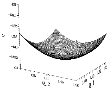
FIG. 48.: The potential energy surface $V$ for scenario 1 corresponding to the temperature $T=1$ at equilibrium. The unit for the collective coordinates is $0.005$.

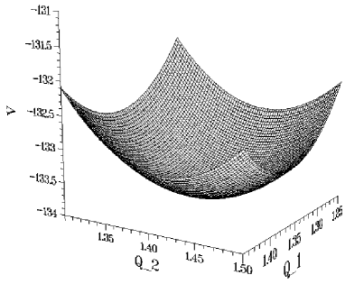
FIG. 49.: same as for Fig. 48 for scenario 2.

Fig. 48 and Fig. 49 give the potential energy surfaces for $T=1$ for the two scenarios. Aside from the equilibrium point, there is no one-to-one correspondence between the coordinates $Q_{1},Q_{2}$ for the two scenarios because one corresponds to a fixed $T$ while the other to a fixed set of values of $R_{3},S_{3}$. Notice that, for scenario 2, the equilibrium point, for non-zero temperature, is not the point of lowest value of the potential energy, but instead is the minimum of the free energy $F=V-ST$.

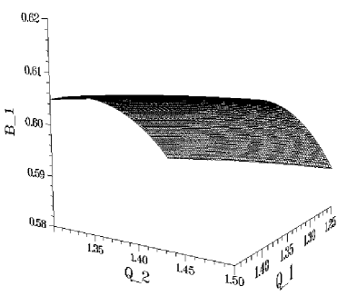
FIG. 50.: The inverse mass $B_{1}$ for scenario 1 for $T=1$.

In Fig. 50, we display the inverse mass function $B_{1}$, which is seen to be a smooth, slowly varying function of the coordinates. This provides some justification for the approximations we have made in deriving the final equations of motion. See also the discussion in reference to Fig. 53.

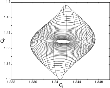
FIG. 51.: The trajectory in coordinate space up to time $t=25$.

Figure 51 shows the trajectory of the system point. It starts from the equilibrium point and after a long time will return at the end (we stop the calculation at $t=25$) to the same point which, as said above, is the one with lowest free energy.

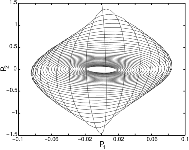
FIG. 52.: Evolution of the momenta.

Figure 52 shows how the momenta are transferred from one mode to the other. This motion will also stop after a long time. Figs. 51 and 52 are obtained for scenario 2. Both figures demonstrate that we are dealing with underdamped motion, which was to be expected, since for our derivation to be justified the frictional forces must be weak compared to the conservative forces. At this point it is necessary to explain why our equations predict that the system returns to its original starting temperature rather than to a higher one resulting from the dissipation of collective kinetic energy. First we shall prove that it does so, and then we shall explain where this energy has gone.

Consider first scenario 1, where we have not displayed the figures corresponding to Figs. 51 and 52, but where the end results are the same. The adiabatic collective manifold is defined by the variables $Q_{a}$ and the entropy $S$, given as a function of the occupation numbers for our model by the formula,

$$S=-\sum_{a\pm}[n_{a\pm}\ln(n_{a\pm})+(1-n_{a\pm})\ln(1-n_{a\pm})].$$ (721)

It is important to emphasize that though in general the $n_{a}$ can change, as long as $S$ remains constant, the mean-field approximation limits matters further to fixed sets of $n_{a\pm}$ determined by equilibrium configurations (in order to guarantee that $R_{3}$ and $S_{3}$ remain constant). Recall as well that the allowed values of $n_{a}$ are associated with equilibrium temperatures, $T_{{\rm eq}}$, and we might further put the same subscript on $S$ to emphasize the restriction on permitted values of $n_{a\pm}$. We visualize the collective manifold by associating with each macroscopic function a surface in $Q_{1}$, $Q_{2}$ with each value of $S_{{\rm eq}}$ or, equivalently, $T_{{\rm eq}}$. Figure 48 is such a representation for the mechanical energy, $V_{\mathrm{C}}$, which for our system may also be identified as the internal energy when expressed as a function of the $Q_{a}$ and $S$, whose minima determine the equilibrium values of $Q_{a}$.

Now consider the relaxation phenomenon. To be able to compare results for the two scenarios we have chosen identical initial conditions – equilibrium values of variables defining the collective submanifold and an initial collective kinetic energy. The system dissipates the kinetic energy as it also moves through non-equilibrium values of $V_{\mathrm{C}}$. But in this mean field approximation it must at all times maintain the initially assigned value of the equilibrium entropy. Therefore when it returns to equilibrium, it returns to the equilibrium configuration of the coordinates associated with the initial occupation numbers, namely the initial temperature.

Where has the collective kinetic energy gone? The answer is, in fact, trivial and could have been given without going through the thermodynamic argument of the previous paragraph. We simply have to remember that according to Eqs. (710a) and (710b), we are describing equilibrium by a canonical distribution, and therefore we have put the system into contact with a heat bath at temperature $T$. Consequently whenever we disturb the system from its equilibrium point simply by a collective kick (collective kinetic energy), this energy will eventually dissipate to the heat bath and the system return to its original equilibrium thermodynamic state. But this implies that as long as we displace the system from equilibrium with the given choice of initial conditions, the final state will be the same independent of the choice of scenario, i.e., independent of the choice of master equations, and should hold for any choice of master equations that have the canonical distribution as their static solution.

Matters are slightly more complicated if we start the system at a point with non-equilibrium values of the coordinates $Q_{a}$. In the mean field scenario, we must,nevertheless, choose values of $R_{3}$ and $S_{3}$ that correspond to a common temperature, which is the final equilibrium temperature. For scenario 2, we must specify a starting local temperature and let the dynamics tell us the final equilibrium temperature.

FIG. 53.: Variation of the total collective energy $W_{\mathrm{C}}$ for the two scenarios.

Figure 53 gives the evolution of the total collective energies $W_{\mathrm{C}}$ for the two scenarios. The evolution is not quite the same but the near overlap of the two curves means that the total spaces (including the temperature) are almost identical. This may be understood by noting that the latter are defined starting from the same equilibrium points and furthermore that we are looking at the motion close enough to these points. The curves have been obtained using Eq. (706). We checked that the same values are obtained by direct integration of Eq. (707). This reflects the fact that the inverse mass functions are weakly coordinate dependent. Figures 51,52,53 all show the dissipative character of the motion.

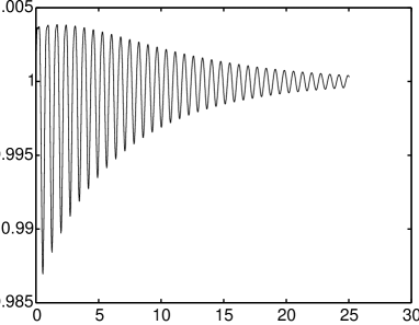
FIG. 54.: Variation of the temperature $T$ with time.

Finally, Fig. 54 exhibits the variation of the temperature $T$. It starts from $T=1$ and ends up at the same value when the motion stops. The quasi-periodic structure of the curve reflects the underdamping. One should not be surprised by the fact that local temperatures dip below its equilibrium value. This can be understood as a consequence of Eq. (713). Most simply, if we had reversed the sign of the initial momenta, the system would have moved immediately in the direction of smaller local temperature.

In summary, we have made a number of compromises in the treatment of our model that suggest further studies to circumvent these limitations. The simplest that comes to mind is to investigate the dynamics of the self-contained system without introducing the white-noise approximation. For example, we can study the initial-value problem in which the initial energy resides completely in the collective subspace. We then integrate the equations of motion to examine the flow of energy between that space and the non-collective space as the number of oscillators in the latter is increased. We expect to find that for a sufficiently large non-collective space the collective energy all dissipates eventually, and we may even be able to extract effective frictional constants to describe average effects of this process. For an initial study, it would suffice to take a simple Lipkin model in the mean-field approximation.

VII Survey of literature and summary

A Survey of literature

In making the decision to write this review completely from the unitary point of view of the authors, we have slighted a rich development. Much of this took place in the decade preceding our initial efforts in the field. However, research of sometimes considerable depth, if with narrower participation, has continued to the present. The discussion which follows represents our attempt to redress this imbalance. We shall attempt a survey of the literature, that is relatively complete in its attributions, but relatively sparse on specific details. From our narcissistic point of view, we can divide the literature into three compartments, papers that have had an impact on the field as a whole but very little influence on our own efforts, papers not widely noticed that have been helpful to us, and work that is both well-known and has been inspirational to us. In the course of the survey that follows, we shall try to acknowledge indebtedness in so far as we are aware of it.

Though their approach has never been brought to full fruition in the sense in which it was originally envisaged, the work of Baranger and Veneroni [8] (the publication of their full report occurred a number of years after their work was already widely known) must be credited with stimulating much of the extensive activity and development that took place in this field over a period of more than a decade. Their special contribution was to introduce a new decomposition of the density matrix, $\rho(t)$, associated with time-dependent Hartree-Fock theory into time-even and time-odd parts that could be identified as canonical coordinates and canonical momenta, respectively, in the adiabatic limit. Specifically, they introduced the decomposition

$$\rho(t)=\exp[i\chi(t)]\rho_{0}(t)\exp[-i\chi(t)].$$ (722)

Here $\rho_{0}(t)$ is a time-even Slater determinant appropriate for the description of the unconstrained equilibrium shape of a system with an even number of nucleons, or of the conditional equilibrium shape achieved when shape constraints are imposed. In the adiabatic limit, the exponential factors can be expanded, and it is then shown that the Hartree-Fock equations have the form of Hamilton’s classical equations of motion with the matrix elements of $\rho_{0}$ serving as coordinates and those of $\chi$ as canonical momenta. However the authors do not reach the concept that the introduction of collective coordinates can be associated with a canonical transformation, nor do they formulate a useful algorithm for the construction of the collective subspace. They do suggest a time-dependent calculation designed to identify collective behavior. In a useful paper [48], to which we shall return, Goeke, Reinhard, and Rowe describe this procedure, but find that it does not work when applied to a simple (non-nuclear) model. We quote without discussion other papers that have studied some aspects of adiabatic TDHF theory using the decomposition (722) [131, 132, 133, 134].

This decomposition was also studied further in Ref. [135], in which it is pointed out that the decomposition (722) is a useful starting point for the derivation of the hydrodynamic limit of TDHF. Some of the authors of the latter report made an extensive effort to apply their ideas. The outcome of this effort [136, 137, 138] was a method of computing what we have called the covariant collective mass without having to invert the given contravariant mass tensor, sometimes a formidable task in the nuclear physics context. This method is known as the double cranking method, and was suggested earlier, e.g., by Villars [139], though not previously implemented. We outline the essential steps of this method. We first remind the reader that to first order in the collective momenta, the decoupling conditions have the form

$${\cal H}_{ph} = -i\rho_{ph}^{1i}\partial_{i}V=\frac{\partial Q^{i}}{\partial\rho_{hp}}=f^{i}_{ph}\lambda_{i},$$ (723)

$$B^{php^{\prime}h^{\prime}}f^{i}_{ph} = B^{ij}\partial_{j}\rho_{ph},$$ (724)

$$B^{ij} = f^{i}_{ph}B^{php^{\prime}h^{\prime}}f^{j}_{p^{\prime}h^{\prime}}.$$ (725)

 

In passing, we describe a global method for (possibly) solving these equations that is distinct from any that we have proposed previously. First solve the cranked Hartree-Fock equation (723) with prescribed cranking operators $f^{i}_{ph}$. This yields a density matrix $\rho(Q^{i})$, from which derivatives with respect to $Q^{i}$ may be computed. From (725) a trial value of $B^{ij}$ may be obtained. Thus a trial value of the right hand side of (724) is known. By inverting the matrix $B_{php^{\prime}h^{\prime}}$ we thus obtain improved values for the cranking operators,

$$f^{i}_{ph} = B_{php^{\prime}h^{\prime}}B^{ij}\partial_{j}\rho_{p^{\prime}h^{\prime}}.$$ (726)

We can now cycle back and forth between (723) and (724) until convergence is hopefully achieved. It should be noted, however, that in a test calculation in Ref. [48], using the landscape model, convergence could not be achieved with this method.

 

Now suppose we want to do a calculation without full self-consistency, in particular one with prescribed cranking operators, chosen on the basis of physical plausibility, as has been the case for most of the history of the subject. The question that arises is how we should compute the collective mass tensor. The formula (725), using the prescribed cranking operators is not sufficiently accurate since it does not, in general, contain the (self-consistent) cranking limit. The alternative formula for the covariant mass tensor

$$B_{ij} = \partial_{i}\rho_{ph}B_{php^{\prime}h^{\prime}}\partial_{j}\rho_{p^{\prime}h^{\prime}},$$ (727)

can be shown to be the self-consistent cranking result provided the derivatives $\partial_{i}\rho_{ph}$ are computed from the solution of (723). But this evaluation also requires the calculation of the inverse of $B^{php^{\prime}h^{\prime}}$, and it is precisely the difficulty of this calculation that discourages the application of the self-consistent procedure that involves (726) as the essential step.

The work under discussion avoids the difficulty of inversion (but renounces the goal of self-consistency) by the following procedure. We utilize the formulas

$$\dot{\rho} = \frac{\partial\rho}{\partial Q^{i}}\dot{Q^{i}}+\frac{\partial\rho}{\partial P_{i}}\dot{P}_{i}$$ (728)

$$\frac{\partial Q^{i}}{\partial\rho_{hp}} = -i\frac{\partial\rho_{ph}}{\partial P_{i}},$$ (729)

the second of which will be recognized as a canonicity condition previously utilized, and apply the equation of motion for $\dot{P}_{i}$. As a consequence the TDHF equation, in the representation in which $\rho$ is diagonal (working always to first order in velocity or momentum), takes the form

$${\cal H}_{ph}-\lambda_{j}f^{j}_{ph}-i\dot{Q^{j}}\partial_{j}\rho_{ph}=0.$$ (730)

This equation may be called a double cranking equation with cranking parameters $\lambda_{i}$ and $\dot{Q^{i}}$. It can be solved as follows: First set $\dot{Q^{i}}$ to zero, so that we have the usual single cranking. From the solution of this problem, we calculate $\partial_{i}\rho_{ph}$, which defines the cranking operator associated with the Lagrange multipliers $\dot{Q^{i}}$. For each value of $Q$ (suppressing indices) we then crank on the velocity. We thus obtain $\rho(Q,\dot{Q})$. For small $\dot{Q}$, this should have the form

$$\rho(Q,\dot{Q}) = \rho(Q)+\frac{\partial\rho}{\partial\dot{Q^{i}}}\dot{Q^{i}},$$ (731)

$$\frac{\partial\rho_{ph}}{\partial\dot{Q}^{j}} = \frac{\partial\rho_{ph}}{\partial P_{i}}\frac{\partial P_{i}}{\partial\dot{Q}^{j}}=if^{i}_{ph}B^{ij}.$$ (732)

From (732) we can calculate $B^{ij}$. The results of this formulation have been applied to the study of isoscalar quadrupole modes in light nuclei.

In this method, the collective coordinate is prescribed, but the associated canonical momentum is determined from the calculation. Because full self consistency is not attempted, the choice of collective pair is not optimal.

The utility of deriving conditions for characterizing large amplitude adiabatic collective motion by solving the TDHF equations as a power series in the collective momenta was first recognized by Villars [77]. In his work, he derived the TDHF version of the three decoupling conditions, namely the force, mass, and curvature conditions. However, he was ambivalent about the curvature condition, emphasizing correctly that to second order in the momentum, extended point transformations would have to be considered. Since he confined his attention to point transformations, he felt that the inclusion of this condition was inconsistent. The equations he adopted are therefore summarized in (723)-(725). The global method he suggested for solving these equations is precisely that described above. As already stated this method was tested on a simple model in [48] and shown to be unstable. Stabilization is achieved by converting these equations into the LHA. This conversion has been described repeatedly in this work, and is one of the foundations of our program. In a further paper [83], the theory was extended to include coupling between the collective and the non-collective spaces.

The influence of the concepts introduced by Villars on our own work is manifest. Together with the less well-known papers [42, 43] which emphasize the clarity that can be achieved by first considering large amplitude collective motion within a purely classical framework, this work has provided the theoretical framework within which our development is contained.

Among the works also based on an expansion of TDHF in powers of the collective momenta, we shall discuss the theoretical formulation of Goeke, Reinhard, and their collaborators [140, 141, 142, 48]. These authors also adopt as their basic equations the zero and first order conditions (723) and (724). By eliminating $f^{i}_{ph}$ between these two equations, they obtain the condition

$$B^{php^{\prime}h^{\prime}}{\cal H}_{p^{\prime}h^{\prime}}=\lambda_{i}B^{ij}\partial_{j}\rho_{ph}.$$ (733)

For the case of a single collective coordinate, the right hand side of (733) becomes a constant times $\partial_{Q}\rho_{ph}$. The constant can be absorbed into the scale of $Q$, and thus we obtain a first-order differential equation to determine a change in the density matrix when we change $Q$ by a small amount. However, if our starting point is not on a collective path, the one-dimensional manifold that we generate will not be the optimized path we seek. To find a suitable starting point, the authors formulate a validity criterion specifying that such a point should approximately satisfy the condition of second order in the momentum that emerges from the fundamental analysis. They also show how to solve (733) in such a way that starting at an arbitrary point, one can descend to a point on the collective path. They have applied this method with reasonable success to a number of examples of ion-ion scattering at low energies [143, 144, 145, 146, 147, 148]. The agreement with experiment is improved if some quantum corrections, obtained by the method of generator coordinates, are included. The application of this method to the theory of large amplitude collective motion will be discussed below.

A second body of work to which we are indebted is that of Rowe and collaborators [149, 45, 150]. The first of these papers contains, as far as we know, the first formulation of the LHA without curvature, associated with a stable local method for obtaining a solution that we have, in effect, utilized in our work. The second paper cited is a careful mathematical analysis of the properties of valleys and fall lines (lines in the direction of the gradient of the potential) and a proof of why the curvature criterion of Goeke and Reinhard, mentioned above, is relevant for the determination of the collective path. Our formulation of the concept(s) of multi-dimensional valleys came after a study of this work. The purpose of Ref. [48] was to illustrate the various methods, then known, for constructing a collective path. After definitions of the proposals of Rowe-Basserman (LHA), Villars, Goeke-Reinhard (GK), and Baranger-Veneroni, these are all applied to the landscape model in two dimensions, from which one aims to decouple one collective mode. As discussed above, only the LHA and the method of GK “work”. The former can be applied to decouple a collective manifold of any dimensionality (in principle), but the latter is restricted in its application to one collective coordinate.

The idea of an expansion in powers of the momentum was also used effectively later in the work of Mukherjee and Pal [151, 152], who actually showed that the three decoupling conditions implied that a decoupled path must be a valley. This work was very influential on our own thinking, though in strict mathematical terms, it is a paraphrase of the earlier result of Rowe [45], who remarked that geodesic fall lines are decoupled. In the language of this review, this means that a path that satisfies the mass and force conditions and is also geodesic is decoupled, since the last condition is equivalent to also satisfying the curvature condition. Later work by these authors [153, 154, 155, 156, 157] is both contentious and displays no real conceptual advance compared to the earlier work. For example, these authors never realize that a decoupled manifold is perfectly well-defined by the LHA, except that it is not a valley unless the curvature is included. Also they never reached the conception that the theory as formulated applies perfectly well to a multi-dimensional collective manifold.

We turn next to the accomplishments of Marumori, Sakata, and their associates [158, 159, 160, 161, 162, 163, 164]. One can find in their work the analogues of many of the concepts described in this review: exactly and approximately decoupled manifolds, goodness of decoupling condition, and stability condition, though the terminology is often different from the one we use. Except for their early work, which emphasized a concept called the “Invariance Principle of the Schrödinger Equation”, in practice a special treatment of the variational principle for TDHF, the development has been parallel to ours, as we have always emphasized. (Their silence in this regard has, on the other hand, been deafening.) The algorithm associated with their work, the self-consistent coordinate method (SCCM), is local harmonic, closely tied to the TDHF formalism, and designed to obtain a collective Hamiltonian to describe anharmonic vibrations. Applications by these authors have been limited to schematic models, but, as we shall discuss below, realistic applications of SCCM have been carried out by others. Also, one of the present authors was involved in an independent development of some of the early ideas of Marumori within a completely quantum framework [165]. An interesting comparison between the approaches by Sakata and Marumori, Goeke and Reinhard, and that by Rowe, can be found in Ref. [166], which should be compared to our own work in Ref. [28].

In their later work, which diverges completely from ours [167, 168, 169, 170, 171, 172, 173, 174, 175, 176, 177, 178], they undertook the program of studying TDHF as a non-separable Hamiltonian system with the aim of incorporating advances in the understanding of chaos into the nuclear problem. They identified the occurrence of resonant conditions under which the perturbative construction of the series of anharmonic terms failed to converge. Subsequently they modified their theory to take into account the transfer of energy between the collective and these special non-collective degrees of freedom. Finally, they have developed a version of transport theory to deal with this class of problems. The connection of their work to the more restricted considerations presented in Sec. VI is not apparent.

Important theoretical contributions and some elementary applications have also been carried out by Yamamura and Kuriyama. In one series of papers [179, 180, 181, 182, 183, 184], they have also exploited the canonical structure of TDHF and the essential role of canonical transformations to introduce collective and intrinsic variables. Their work is, however, still tied to the SCCM of Marumori, Sakata, et al and to the anharmonic limit; no algorithm applicable to large amplitude collective motion is given. In subsequent work [185, 186, 187], they have carried through a deeper mathematical study of the same set of ideas. All this work plus other uses of TDHF are reviewed in Ref. [187], where one also finds a few applications. Following this work, the authors, in collaboration with J. da Providencia, undertook to investigate, using the methods of thermo field dynamics [121], the application of TDHF to systems at finite excitation energy. The development may be traced from Refs. [188, 189, 190, 191], which represents the part of the research most closely related to LACM.

The TDHF method in an expansion about equilibrium (and ultimately the SCCM) have also been applied to the study of the wobbling motion of a triaxial rotor by Kaneko [192, 193, 194]. A related approach is discussed by Marshalek [195].

We emphasize the parallelism of the basic theoretical structure in the works of Yamamura and Kuriyama, of Marumori and Sakata, and of our own efforts. Because of the way we have developed these ideas, both theoretically and practically, the superficial reader may, however, encounter difficulty in recognizing the overlap of ideas.

As already emphasized, there have been no applications of any of the theories referred to in the paragraphs immediately preceding to large-amplitude collective motion. However, the SCCM, which is a classical method for anharmonic vibrations that requires requantization, has been applied very successfully to gamma vibrations of deformed nuclei [196, 197, 198, 95, 199, 200]. It has also been applied to collective-noncollective quadrupole coupling (anharmonic vibrations in the single-j shell model [201], to the description of two-phonon states in Ru and Se [202], and most enticingly [98], in work that cries for further study and extension, to a comparison of the diabatic versus the adiabatic approximation. The model found in this reference has been studied by our techniques in Ref. [36], of which no account has been included in this review. On the other hand in Sec. IV E 1, we have reviewed a study of a more general model incorporating similar concepts. In the study of gamma vibrations, particular attention was paid to the ambiguities of requantization, to the nature of the mode-mode coupling responsible for the anharmonicity in the gamma mode, and to the restoration of number conservation. Finally we mention [203] an application of SCCM to the spherical to deformed phase transition in the Sm isotopes. Since this method cannot deal with arbitrary large-amplitude distortions, the problem was studied by expanding to fourth order in the quadrupole coordinates and momenta. Such a Hamiltonian is rich enough to describe a phase transition; whether it is sufficiently accurate remains to be seen.

An elegant but formal study of the description of decoupled manifolds within the framework of time-dependent Hartree-Bogoliubov theory and a group structure dictated by the nuclear shell model has also been carried out by Nishiyama and Komatsu [204, 205, 206, 207, 208]. Though they make no use of the canonical structure, their basic approach can be understood by reference to the results found in Sec. II C of this review, if we identify the local harmonic equation developed there as integrability conditions for the consistency of the decoupling conditions. We have emphasized how the two sets of equations, consistency conditions and decoupling conditions, must be solved in concert to provide integral surfaces that are candidates for decoupled manifolds. In the work cited [208], only the power series option is suggested.

The concept of an approximately decoupled manifold occurs very naturally in the description of chemical reactions. In an adiabatic description, one can think of the reaction as involving the passage from a local minimum of the total potential energy of the reactants through a transition state that corresponds to a saddle point of the potential energy and then down to another local minimum corresponding to the final products. The reaction is thus described classically by a reaction path, corresponding to a one-dimensional approximately decoupled manifold [209]. An approximate Hamiltonian for the system, often sufficient for studying the given reaction, can be obtained by expanding the full Hamiltonian about the reaction path and retaining quadratic terms (the small oscillation approximation). The procedures to be found in the chemical literature differ only in the way the reaction path is determined. The literature on this subject is vast, but can be traced from the papers to be cited. Most of the work [209, 210, 211, 52, 212, 213] is based on a reaction path chosen as the fall line (direction of the gradient of the potential) in both directions from the saddle point. Thus there is a remarkable similarity to the method of Goeke and Reinhard described above. Quite recently several alternatives have been proposed. One method, the gradient extremal method [214, 215], is tantamount to the LHA with the neglect of curvature corrections. A second proposal [216] is to use a suitably chosen straight line path of descent from the saddle point to each of the minima. This proposal is relevant to the situation that the fall line has large curvature, rendering it unlikely that the system will follow such a path. In this method, the kinetic energy can be brought to diagonal form. This means that the mass and curvature decoupling condition has been satisfied, at the expense, however, of a violation of the force condition.

Several field-theoretical applications of LACM techniques have also been studied, in particular to tunneling phenomena, and to the construction of collective coordinates for solitons. The treatment of tunneling is discussed in a recent review [217], where a valley approach is used, but in the action rather than in configuration space. The idea of using the LHA to generate the collective coordinates has been applied in Refs. [218, 219] to the Skyrme model. It was found to be a useful approach in the study of parts of the collective manifold.

So far, all the work in nuclear physics quoted in this section has been based on TDHF theory. Remarkably the first published derivation of the LHA, that of Holzwarth and Yukawa [71], was based on the generator coordinate method (GCM). In this method, we represent an eigenstate of the many-body system in the form

$$|n\rangle = \int dCF_{n}(C)|C\rangle,$$ (734)

where $|C\rangle$ represents a continuous set of Slater determinants parameterized by a set of generally complex coordinates $C$ (or real pairs $Q,P$). Historically, the need for this doubling was discovered by the application of this method to the problems of translational motion and to the rotational motion of deformed nuclei [220]. For the translational problem, for example, it was necessary to superpose not only determinants centered at different points (center of mass coordinate), but also to allow determinants with a continuous distribution of momenta of this center of mass. Only then was it possible to extract from (734) translational motion with the correct total mass. The general need for this doubling was first fully explained in the works of Dobaczewski [221, 222].

In the traditional application of the GCM to the study of collective motion, the manifold of states $|C\rangle$ is assumed known and the state (734) is considered as a trial function leading to the well-known Hill-Wheeler [105] integral equation for $F_{n}(C)$. To be specific, consider the quadrupole degrees of freedom studied in the Kumar-Baranger theory [1, 2, 3, 4, 5]. For this and for more modern applications, the latter has been replaced by a two-step procedure [88, 89]. In the first step, one constructs the required manifold $|C\rangle$ as the solution of a constrained HF + BCS problem with so-called time-even, i.e., velocity-independent, constraints, such as the quadrupole moment and selected higher moments. This parallels the first step of the KB theory, except that more realistic forces fitted to ground-state properties are utilized. In the second step, one solves the Hill-Wheeler equation. Compared to the procedures described in this review, and in the bulk of the work noted in this section, it has the advantage that no adiabatic approximation is necessary and thus application to large-velocity phenomena is less questionable. On the other hand, the description of the large-amplitude collective motion is not self-consistent in our sense. Furthermore, there remains a question whether inertial properties of the collective degrees of freedom are correctly described by this method, since we know from the simpler examples of translation and rotation that in such cases the manifold $|C\rangle$ needs to be constructed from a double cranking procedure utilizing one velocity dependent constraint for each collective degree of freedom. Nonetheless, an approach exists to construct a collective potential and mass parameter from the GCM that has been widely applied, see, e.g., [223, 224].

Returning to the work of Holzwarth and Yukawa, these authors extended the use of the state vector (734) as a trial function by varying not only the “wave function” $F_{n}(C)$, but also by varying the manifold $|C\rangle$ so as to optimize its choice for each value of the set $C$. Their argument, which we shall not reproduce, leads to the LHA without curvature. Further study of the ideas introduced by HY has been carried out by Goeke and Reinhard [225, 226, 76]. Basically they have shown that if one applies the generator coordinate method to the space of Slater determinants that contains both even and odd members, parameterized by pairs of canonical coordinates, then by a suitable expansion in powers of the momentum one essentially reaches the results obtainable from TDHF by a momentum expansion. There is an additional bonus that zero point fluctuations associated with the collective coordinates can be computed; these were incorporated in the applications to which we have previously alluded [142, 143, 144, 145, 146, 147, 148].

For completeness, we remark on the occurrence of two sets of researches on problems of large amplitude collective motion that utilize the path integral method. One set involves H. Reinhardt and collaborators (see the review in Ref. [227]), and comprises two papers on the application of PIM to simple solvable models [228, 229], two formal papers deriving a theory of large amplitude collective motion [230] and a theory of fission [231], and finally, one paper [232] showing how to extract adiabatic TDHF by the path integral method. In the work of Levit, Negele, et al, we encounter a formal development [233, 234], which then concentrates on the problem of fission [235], culminating in a method of solution that showed considerable promise [236, 237].

In Sec. V of this review, we have presented our version of what may be termed the nuclear BO method. In this presentation, the basic ideas have a clear association with the corresponding concepts utilized in molecular physics. On the other hand our aim was to embed the results previously derived from TDHF into a quantum framework. The only other attempt to study large amplitude collective motion by a BO method was the prior work of Villars [238]. The differences between this work and ours appear to be greater than the similarities. We both use basis vectors in Hilbert space associated with localized collective and intrinsic operators. Villars uses an expansion of the Hamiltonian in terms of collective momenta that is an operator equivalent of the moment expansion. (We had, in fact noted this relationship a long time ago [239]). On the other hand the treatment of state vectors in [238] is faintly redolent of the Hill-Wheeler representation. Villar’s ideas have been applied with success to an exactly solvable model [240] and to a fresh theoretical study of rotations and vibrations [241].

We have also studied the effects of the BO approximation and the role of the induced gauge fields, which are related to (avoided) level crossings. This area of physics has a long history, and is already discussed in old work by Brink [242]. An interesting modern perspective, in a framework similar to ours, can be found in the work of Bulgac and Kusnezov [243, 244].

B Summary of concepts and results

This review has been devoted first to the study of some properties of a classical Hamiltonian at most quadratic in the momenta with a non-singular coordinate-dependent mass tensor. After an elementary introduction, the theoretical structure upon which most of the applications have so far been based was developed in Sec. II. The most general canonical transformation that maintains this structure exactly is a point transformation; in so far as we restrict ourselves to such transformations, we are within the realm of Lagrangian dynamics. On the other hand, if we view the Hamiltonian as an approximate one resulting from an expansion of the exact Hamiltonian in powers of the momenta (adiabatic approximation), and think of a general canonical transformation similarly expanded, it is necessary to go one step beyond strictly point transformations to assure that final results do not depend on a particular initial choice of canonical coordinates. For want of a better term, we referred to such (approximate) canonical transformations as extended point transformations.

Consider first strictly point transformations. Our aim was to discover if the given Hamiltonian admits motions confined to a submanifold of configuration space, called a decoupled manifold. The idea of such motions both generalizes the concept of separability and, for the case of a many-particle system, provides a natural definition of collective motion for systems where the original choice of coordinates corresponds to single-particle degrees of freedom. A parameterization of the manifold is provided by a subset (the collective subset) of a new set of coordinates introduced by a point canonical transformation, though it becomes immediately evident that any single choice of coordinates is not unique, the only invariant being the geometric structure itself.

Our first strategic contribution was to insist on the separation of two sets of problems, one theoretical and the other practical. The first is that of stating precisely the conditions for a decoupled Lagrangian manifold to occur. There we found it necessary to distinguish between the case that none of the collective momenta is conserved and the case that one or more is. In the former instance, that engaged our full attention first, we found three conditions, of order zero, one, and two in the collective momentum, christened force, mass, and curvature condition, respectively. The mass and curvature conditions require that an exactly decoupled manifold be geodesic with respect to the mass tensor as metric. Stimulated in part by previous work, that we have generalized, we found three transformations of these conditions into exactly equivalent sets of conditions. In the first presented, the generalized valley formulation, the curvature condition was replaced by an infinite set of generalized force conditions. In the second transformation, we proved that the curvature condition can be replaced by an eigenvalue problem that generalizes the usual random phase approximation, reducing to it at critical points of the potential energy. This was called the Riemannian local harmonic formulation to distinguish it from the third formulation, the symplectic local harmonic formulation. In the latter it was shown that the force and mass conditions alone imply a different eigenvalue equation that replaces only the mass condition. The revisions of the formulations necessary when extended point transformations and/or additional constants of the motion must be considered were described rather more briefly than for the case considered above.

Most Hamiltonians do not admit exactly decoupled manifolds. Yet the phenomenon of approximately decoupled collective motion is observed widely. From the point of view of the present work, these are motions that remain in some neighborhood of a submanifold either for a very long time or possibly forever. To uncover such manifolds, we described two different constructions or algorithms that provide submanifolds of preassigned dimensionality $K$ (in practice $K=1$ or 2). The nature of these manifolds must be such that they are exactly decoupled if the given Hamiltonian admits such motions. This was guaranteed by the way in which each algorithm is related to an associated formulation. Consider, for example, the one associated with the generalized valley formulation. Recall that the latter requires that an infinite number of generalized forces lie in the tangent plane to the decoupled manifold. In the algorithm, we replaced these consistency conditions by a well-posed problem, namely, we defined a candidate surface of dimension $K$ to be the locus of points at which the “first” $K+1$ generalized forces determined a plane, generally distinct from the tangent plane. Various goodness-of-decoupling criteria suggested depend on the relative orientation of this plane with respect to the tangent plane, the two planes coinciding at each point if the decoupling is exact.

The second algorithm was based on the local harmonic formulations, which require that the basis vectors of the tangent plane can chosen as eigenvectors of a second covariant derivative of the potential energy, the force itself being required as well to lie in this plane. The problem becomes well-posed when the plane attached to each point of a manifold, as determined from the solutions of the local harmonic equation, is not required to be tangent to the manifold. We showed, however, that for numerical purposes this algorithm could be formulated as a variant of the GVA. As illustrated in the numerical applications, different algorithms give different approximate results, with exceptions as noted.

In addition to testing for goodness of decoupling, one must also test for local stability of motion. The latter is the more-or-less standard calculation, the same for both algorithms, of frequencies of small oscillation in directions normal to the manifold, to verify that they are real. In general such frequencies are position-independent only in the special case of separable motion; an imaginary frequency signals that $K$, the dimensionality of the collective subspace, must be increased.

Section III contains first applications of the general formalism to several problems involving only a few total degrees of freedom. As a general characterization, we may refer to these applications as the approximate quantization of non-separable systems, in which we attempt, successfully in all the examples considered, to decouple one or two collective coordinates from a system with just a few additional degrees of freedom. These applications include schematic models of nuclear fission and chemical isomerization. It is clear that much more development and application can be done along these lines.

However, in Sec. IV we turn to the problem that stimulated the theory in the first place, the interest in LACM in nuclear physics. These applications are based on TDHF where pairing can be neglected and on TDHFB where it cannot. Our ability to apply the theory of Sec. II to these problems is based on the well-known property of these approximations that they can be shown to have the classical Hamiltonian structure. The formulas necessary for applications are first developed and then applied to three sets of problems. We first successfully solve an exactly solvable model of monopole vibrations and show how non-solvable extensions can be studied. We then devote considerable attention to a study of the low lying spectrum of ²⁸Si. For reasons that have to do with the model chosen – the size of the configuration space and the form of the Hamiltonian – the results of this investigation are only partially satisfactory. Finally, in our third application, we lay the basis for a realistic treatment of heavy nuclei designed to generalize the KB theory. In the light of the results of this preliminary investigation and the remaining contents of the review, this opens the most promising path for realistic applications.

The theory developed in Sec. II is a classical theory. The applications to quantum mechanics are based on a requantization of a classical collective Hamiltonian. In the course of our studies, we also remark on how to include the next order of quantum corrections, which involve oscillations of the non-collective coordinates. For the nuclear case, with its Fermi-Dirac statistics, this involves a non-trivial new development whose results we have quoted and applied. Both for the chemical isomerization discussed in Sec. III and for the case of Si, these corrections are of considerable importance. In Sec. V, we consider the basic theory anew, from a quantum-mechanical viewpoint based on the study of the equations of motion within the framework of a Born-Oppenheimer approximation. In addition to regaining old results, we are able to incorporate the effects of the Berry phase into our treatment. Several simplified models that incorporate this new physics are worked out, but the inclusion in realistic applications remains a task for the future.

Our final contribution, in Sec. VI, describes the generalization of the theory of LACM to finite excitation energy so as to describe the exchange of energy between collective and non-collective coordinates. Though a formal structure has been elucidated and applied to a simple model, it is clear that much more work is required before we can hope to apply this theory to realistic cases.

We add a few words about future prospects. The main reason for optimism concerning the immediate future of our subject is that the ideas explored in Sec. IV for heavy nuclei indicate that the class of problems that stimulated the researches in this field in the first place, the low-energy spectroscopy of deformed and transitional nuclei, is finally amenable to an improved treatment compared to previous non-selfconsistent studies.

A Choice of canonical variables in the Hamiltonian formulation of adiabatic time-dependent Hartree-Fock theory

1 Introduction

In Sec. IV A, we have provided a lexicon for the transcription of the Hamiltonian theory of large amplitude collective motion developed in Sec. II into the language of TDHF. In Sec. IV E, we also required a corresponding relationship for time-dependent Hartree-Fock-Bogoliubov theory (TDHFB). In this appendix, we shall survey some of the ways of carrying out this program. The identification can be made both independently of its interest for LACM, using several different choices of canonical variables [53, 54, 55, 56, 57], as well as within the framework of LACM [149, 158, 8, 135, 25]. In our own work, we have utilized either the method developed in Refs. [53, 56, 57] or an even simpler method based on a observation first made in Ref. [25]. Part of the material that follows is based on unpublished work of the authors [245].

Superficially, we can divide the choices into two sets. In one, as in Ref. [55], the canonical variables can be associated directly with time-dependent single-particle orbitals. In the others, the parameterization is associated with the one-particle density matrix. We shall first address briefly the sets that we do not use, and afterwards go into more detail on those that play a role in our work.

2 Kerman-Koonin variables

We want to recognize the TDHF equations as a form of Hamilton’s equations. It is convenient to start from the variational formulation of the TDHF. The action $S$ has the form

$$S = \int dt\,{\cal L}(t)=\int dt\,\langle\Phi(t)|(i\partial_{t}-H)|\Phi(t)\rangle$$ (A.1)

$$= \int dt\left\{\sum_{h}[\langle\varphi_{h}(t)|i\partial_{t}|\varphi_{h}(t)\rangle-W(\varphi,\varphi^{*})]\right\},$$ (A.2)

where $\Phi(t)$ is a normalized Slater determinant, $\varphi_{h}(t)$ are the occupied single particle wave functions (s.p.w.f.), $H$ is the total Hamiltonian, and $W(\varphi,\varphi^{*})$ is the Hartree-Fock energy for the determinant $\Phi(t)$ and thus a functional of the orbitals $\varphi_{h}(t)$. Only the time dependence is explicitly shown. For applications to nuclear physics, we shall understand here and in future sections that we are dealing with a non-relativistic Hamiltonian of the standard form

$$H = \sum_{a,b}h_{ab}a_{a}^{{\dagger}}a_{b}+\frac{1}{4}V_{abcd}a_{a}^{{\dagger}}a_{b}^{{\dagger}}a_{d}a_{c},$$ (A.3)

where $a_{\alpha},\,a_{\alpha}^{{\dagger}}$ are destruction, creation operators for nucleons in an arbitrary basis of single-particle states and $h$ and $V$ are Hermitian matrices, with $V_{\beta\alpha\gamma\delta}=V_{\alpha\beta\delta\gamma}=-V_{\alpha\beta\gamma\delta}$. Also $h$ may be the kinetic energy, or as is more likely for the applications that we shall carry out, also include a potential term.

The TDHF equations are obtained from the variational principle $\delta S=0$. By varying with respect to $\varphi_{h}^{\ast}$, for example, we obtain the TDHF equation for the orbitals $\varphi_{h}$,

$$i\dot{\varphi}_{h}(t) = {\cal H}(t)\varphi_{h}(t).$$ (A.4)

In the combination of coordinate and spin-isospin labels, summarized as “$x$”, ${\cal H}$ is the integral operator

$${\cal H}(x,x^{\prime};t) = \delta W/\delta\rho(x^{\prime},x;t),$$ (A.5a)

$$\rho(x,x^{\prime};t) = \sum_{h}\varphi_{h}(x,t)\varphi_{h}^{\ast}(x^{\prime},t),$$ (A.5b)

$$W = \mbox{Tr}h\rho+\frac{1}{2}\mbox{Tr}V\rho\rho.$$ (A.5c)

It follows that Eq. (A.4) takes the form

$$i\dot{\varphi}_{h}(x,t) = (\delta W)/\delta\varphi_{h}^{\ast}(x,t),$$ (A.6)

which demonstrates that $\varphi_{h},\varphi_{h}^{\ast}$ are complex canonical coordinates. We decompose these into real coordinates and momenta leading to Hamilton’s equations in real form and to an altered Lagrangian,

$$\varphi(x,t) = \frac{1}{\sqrt{2}}\left(\xi_{h}(x,t)+i\pi_{h}(x,t)\right),$$ (A.7a)

$$\dot{\xi}_{h}(x,t) = \delta W/\delta\pi_{h}(x,t),$$ (A.7b)

$$\dot{\pi}_{h}(x,t) = -\delta W/\delta\xi_{h}(x,t),$$ (A.7c)

$${\cal L} = \sum_{k}\int dx\,\pi_{h}(x)\dot{\xi}_{h}(x)-W(\xi,\pi)+\text{ total time derivative}.$$ (A.7d)

Equations (A.7b) and (A.7c) follow either by transformation from (A.6) and its complex conjugate or by applying the variational principle to (A.7d).

From (A.5b) we compute

$$\rho(x,y,t) =\sum_{h}\frac{1}{2}\left[\xi_{h}(x,t)\xi_{h}(y,t)+\pi_{h}(x,t)\pi_{h}(y,t)\right]$$ (A.9)

$$+\frac{i}{2}\sum_{h}\left[\pi_{h}(x,t)\xi_{h}(y,t)-\xi_{h}(x,t)\pi_{h}(y,t)\right].$$

Therefore the time even part of $\rho$ is real and the time odd part is imaginary.

We shall be interested in the small-momentum limit of (A.9). We thus write

$$\rho(x,y;t) = \rho_{0}(x,y;t)+\rho_{1}(x,y;t)+\cdots$$ (A.10)

$$= \sum_{h}(1/2)\xi_{h}(x,t)\xi_{h}(y,t)$$ (A.12)

$$+(i/2)\sum_{h}[\pi_{h}(x,t)\xi_{h}(y,t)-\xi_{h}(x,t)\pi_{h}(y,t)]+\cdots,$$

$$\rho_{0}^{2}(x,y) = \rho_{0}(x,y)=\frac{1}{2}\sum_{h}\xi_{h}(x)\xi_{h}(y).$$ (A.13)

In lowest order, then, $(1/\sqrt{2})\xi_{a}(x.t),\,a=(h,p),$ are a set of orthonormal functions, and from the equality $\rho^{2}=\rho$ applied to the expansion (A.12) we learn that to first order the expansion of $\pi_{h}(x,t)$ in terms of the complete set $\xi_{a}$ contains only unoccupied orbitals,

$$\pi_{h}(x,t) = \sum_{p}\xi_{p}(x,t)\pi_{ph}.$$ (A.14)

We shall not pursue the physics of these variables any further, since they are not used in this work.

3 Polar representation

Another interesting set of canonical variables is obtained from a polar decomposition of the s.p.w.f.

$$\varphi_{h}(x)=\tilde{\rho}^{1/2}_{h}(x)\exp[i\tilde{\pi}_{h}(x)],$$ (A.15)

with both $\tilde{\rho}^{1/2}_{h}(x)$ and $\tilde{\pi}_{h}(x)$ real.

 

There is an important ambiguity in defining these quantities when the s.p.w.f. $\varphi_{h}(x)$ has nodes. If one chooses $\tilde{\rho}_{h}(x)=|\varphi_{h}(x)|^{2}$, the function $\tilde{\pi}_{h}(x)$ will be discontinuous at the nodes. However, if one defines the phase $\tilde{\pi}_{h}(x)$ as a continuous function, $\tilde{\rho}^{1/2}_{h}(x)$ must change sign at the nodes in order to compensate. Then, $\tilde{\pi}_{h}(x)$ will represent the “real” phase of the s.p.w.f. and will not feature any jumps at the nodes.

 

One way of establishing that $\tilde{\rho}_{h}$ and $\tilde{\pi}_{h}$ are canonical variables is by showing that the Lagrange density (A.7d), when expressed in terms of the new variables, takes the form

$${\cal L}=\sum_{h}\int dx\,\tilde{\pi}_{h}(x)\dot{\tilde{\rho}}(x)-W(\tilde{\rho},\tilde{\pi})+\text{total time derivative}.$$ (A.16)

From this expression it is clear that $\tilde{\pi}_{k}(x)$ and $\tilde{\rho}_{k}(x)$ play the role of canonically conjugate momenta and coordinates for the TDHF problem. Another way is to show that the equations of transformation

$$\xi_{h} = \sqrt{2}\tilde{\rho}_{h}^{{1}/{2}}\cos\tilde{\pi},$$ (A.17)

$$\pi_{h} = \sqrt{2}\tilde{\rho}_{h}^{{1}/{2}}\sin\tilde{\pi},$$ (A.18)

satisfy the Poisson bracket relations. In the small-momentum limit, these equations become

$$\xi_{h} = \sqrt{2}\tilde{\rho}^{{1}/{2}},$$ (A.19)

$$\pi_{h} = \sqrt{2}\tilde{\rho}^{{1}/{2}}\tilde{\pi}_{h}.$$ (A.20)

By comparison with Eqs. (21a) and (22), we see that these are the equations of a point transformation.

The polar representation under discussion can be gainfully employed as a basis for a nuclear fluid dynamical description of collective motion [246], but entering this domain will take us too far afield of our main purposes. The special case that the phase function is independent of orbit, $\tilde{\pi}_{n}(x,t)=\chi(x,t)$ is a special case of the choice of variables studied next, and has been shown to provide an elegant basis for the study of irrotational flow [247].

4 Canonical variables of Baranger and Veneroni

The approach of Baranger and Veneroni (BV) [8, 135] to ATDHF is based entirely on the one body density matrix, $\rho(x,y;t)$. They proved that for any Slater determinant $\rho$ has the unique decomposition

$$\rho=\exp(i\chi)\rho_{0}\exp(-i\chi),$$ (A.21)

where $\rho_{0}$ is a time even operator, and $\chi$ is a time-odd operator. Notice that the equation $\rho^{2}_{0}=\rho_{0}$ imposes no conditions on $\chi$. In fact, different choices for $\chi$ correspond to different physical situations. For example, we have already noted above that choosing $\chi$ as a local operator (point function) is the appropriate choice for the description of irrotational flow. For the study of large amplitude collective motion in the adiabatic limit, the appropriate choice is that $\chi$ have only $ph$ matrix elements in the representation in which $\rho_{0}$ is diagonal, as expressed by the equation

$$\rho_{0}\chi+\chi\rho_{0}=\chi.$$ (A.22)

In the adiabatic limit we consider $\chi$ to be a first-order quantity. In this limit, we now demonstrate that $\rho_{0}(x,y;t)$ and $\chi(x,y;t)$ are canonically conjugate pairs. (As implied by our discussion above, this cannot be true generally.) Here we identify $\rho_{0}$ with the quantity defined in (A.13). Comparing the first-order term of (A.12) with the first order expansion of (A.21), we conclude that

$$\pi_{h}(x,t)=\int dy\,\chi(x,y;t)\xi_{h}(y,t)$$ (A.23)

This allows us to carry out a transformation of the essential kinetic term of the variational principle, as follows

$$\sum_{h}\int dx\,\pi_{h}(x,t)\dot{\xi}_{h}(x,t) = \sum_{h}\int dxdy\,\chi(x,y;t)\xi_{h}(y,t)\dot{\xi}_{h}(x,t)$$ (A.24)

$$= \int dxdy\,\chi(x,y;t)\dot{\rho}_{0}(y,x),$$ (A.25)

which follows if we remember that $\chi$ is a real symmetric matrix. The last form establishes that $\chi$ and $\rho_{0}$ are canonically conjugate in the adiabatic limit.

5 Marshalek-Weneser and Blaizot-Orland variables

From the theorem of Thouless we know that any Slater determinant, $|z\rangle$, that is not orthogonal to a given one, $|0\rangle$, can be written in the (unnormalized) form

$$|z\rangle = \exp[\sum_{ph}z_{ph}a_{p}^{{\dagger}}a_{h}]|0\rangle,$$ (A.26)

$$a_{p}|0\rangle = a_{h}^{{\dagger}}|0\rangle=0,$$ (A.27)

with $z_{ph}$ a set of complex numbers that will serve as variational parameters to derive a version of TDHF. However, as we shall see below, these are not canonical coordinates. Clearly, $h$ refers to the orbitals occupied in $|0\rangle$ and $p$ to the complementary set.

From the definition of the density matrix element,

$$\rho_{ab}=\langle z|a_{b}^{{\dagger}}a_{a}|z\rangle/\langle z|z\rangle,$$ (A.28)

we can derive the formulas (written in terms of a rectangular matrix $z$ composed of the complex numbers $z_{ph}$)

$$\rho_{ph} = [(1+zz^{{\dagger}})^{-1}z]_{ph}=\rho_{hp}^{\ast},$$ (A.29a)

$$\rho_{hh^{\prime}} = [(1+z^{{\dagger}}z)^{-1}]_{hh^{\prime}},$$ (A.29b)

$$\rho_{pp^{\prime}} = [z(1+z^{{\dagger}}z)^{-1}z^{{\dagger}}]_{pp^{\prime}}.$$ (A.29c)

 

We indicate a simple method for deriving these formulas. By utilizing the definition (A.26), the properties (A.27), and the operator commutation relations, one can readily derive the equations

$$\rho_{hh^{\prime}} = \delta_{hh^{\prime}}-\sum_{p}\rho_{hp}z_{ph},$$ (A.30a)

$$\rho_{hp} = \sum_{h^{\prime}}\rho_{hh^{\prime}}z^{{\dagger}}_{h^{\prime}p}.$$ (A.30b)

Together these equations imply (A.29a) and (A.29b). Starting from the definition of $\rho_{pp^{\prime}}$, we can derive a corresponding pair that yield (A.29a) and (A.29c).

 

Turning to the variational principle, we remember that we should utilize a normalized trial function,

$$|\Phi(z)\rangle=|z\rangle/\langle z|z\rangle^{{1}/{2}}.$$ (A.31)

A relatively simple calculation then yields the result

$$\int dt\,\langle\Phi(z)|i\partial_{t}|\Phi(z)\rangle=\int dt\,\frac{i}{2}\mbox{Tr}(\rho\dot{z}-\dot{z}^{{\dagger}}\rho),$$ (A.32)

where $\mbox{Tr}AB=\sum_{hp}A_{hp}B_{ph}$ and the needed matrix elements of $\rho$ are provided by (A.29a)-(A.29c). It can be verified that the equations of motion for $z$ and $z^{{\dagger}}$ that follow from the variational principle are not of Hamiltonian form. (Equation (A.32) does not agree with Eq. (9.118) of Ref. [57]. The result given there follows if one neglects the time dependence of the normalization factor in (A.31).)

A transformation that replaces the matrix $z$ by a matrix $\beta$ that defines canonical pairs is, in fact, well-known [53, 56, 57]. The transformation

$$z=\beta(1-\beta^{{\dagger}}\beta)^{-{1/2}}$$ (A.33)

replaces (A.29a)-(A.29c) by the formulas

$$\rho_{ph} = [\beta(1-\beta^{{\dagger}}\beta)^{{1/2}}]_{ph}=\rho_{hp}^{{\dagger}},$$ (A.34a)

$$\rho_{hh^{\prime}} = [1-\beta^{{\dagger}}\beta]_{hh^{\prime}},$$ (A.34b)

$$\rho_{pp^{\prime}} = [\beta\beta^{{\dagger}}]_{pp^{\prime}}.$$ (A.34c)

Actually Eqs. (A.34a)-(A.34c), as a mapping of density matrix elements onto complex canonical coordinates was first derived as the classical limit of a “boson mapping” from the algebra of all pairs $a^{{\dagger}}a$ to particle bosons, as reviewed in [51].

Defining $|\Psi(\beta)\rangle=|\Phi(z)\rangle$, we can transform (A.32) into the form

$$\int dt\,\langle\Psi(\beta)|i\partial_{t}|\Psi(\beta)\rangle=\int dt\,\frac{i}{2}\mbox{Tr}(\beta^{{\dagger}}\dot{\beta}-\beta\dot{\beta}^{{\dagger}}).$$ (A.35)

This result clearly establishes $\beta$ and $\beta^{\ast}$ as complex canonical coordinates. To apply this choice to LACM, we introduce real canonical coordinates according to the standard equation

$$\beta_{ph}=\frac{1}{\sqrt{2}}(\xi_{ph}+i\pi_{ph}).$$ (A.36)

We then expand the mean field energy to second order in the variables $\pi$ in order to obtain a classical Hamiltonian quadratic in the momenta as a starting point for the theory developed in Sec. II.

The theory developed here can be extended to TDHFB. This extension is carried out in Sec. IV E 2, where it is first needed, and will not be discussed here. We shall instead pass on to our last choice of canonical variables, in some ways simplest of all.

6 Canonical coordinates associated with instantaneous natural orbitals

Consider the TDHF equation

$$i\dot{\rho}_{ab}=[{\cal H},\rho]_{ab}.$$ (A.37)

We choose to study this equation in the representation in which $\rho$ is instantaneously diagonal,

$$\rho_{ab}=\delta_{ab}\delta_{ah},$$ (A.38)

and consider the particle-hole matrix elements of (A.37) in this representation, utilizing (A.38). We thus find

$$i\dot{\rho}_{ph}={\cal H}_{ph}=\delta H/\delta\rho_{hp},$$ (A.39)

that together with the complex conjugate equation identify $\rho_{ph}$ and $\rho_{hp}=\rho_{ph}^{\ast}$ as complex canonical coordinates.

For purposes of application, these variables may be used in a fashion that is quite analogous to what we have described for the variables introduced in the previous subsection. We set (though the left hand side is formally zero)

$$\rho_{ph}=(1/\sqrt{2})(\xi_{ph}+i\pi_{ph}),$$ (A.40)

and expand the mean field energy in powers of $\pi$ to second order in $\pi$ in order to establish a starting point for the theory developed in Sec. II. We state without proof that to this order the variables under discussion are indistinguishable from those introduced in the previous subsection, though this identity will break down in higher order. For this reason, the further development of the theory and applications in Sec. IV utilized the present choice, even though the references on which they are based used the alternative choice.

We conclude this appendix with an account of how the considerations just mentioned can be generalized to the TDHFB. Toward this end we introduce a set of quasi-particle (qp) operators $b_{k}^{{\dagger}}$ related to the particle operators by a general HFB transformation

$$a_{a}^{{\dagger}} = U_{ak}^{\ast}b_{k}^{{\dagger}}+V_{ak}b_{k},$$ (A.41a)

$$b_{k}^{{\dagger}} = U_{ak}a_{a}^{{\dagger}}+V_{ak}a_{a},$$ (A.41b)

$$U^{{\dagger}}U+V^{{\dagger}}V = 1,\;\;UU^{{\dagger}}+V^{\ast}V^{T}=1,$$ (A.41c)

$$U^{T}V+V^{T}U = 0,\;\;UV^{{\dagger}}+V^{\ast}U^{T}=0,$$ (A.41d)

and define the qp vacuum state $|\Psi\rangle$ by the conditions

$$b_{k}|\Psi\rangle=0.$$ (A.42)

To reach our goal as expeditiously as possible, we study the expectation value in the state $|\Psi\rangle$ of the equation of motion for the product $b_{i}b_{j}$. With the definition

$$K_{ji}=\langle\Psi|b_{i}b_{j}|\Psi\rangle,$$ (A.43)

we evaluate the right hand side of the equation

$$i\partial_{t}K_{ji}=\langle\Psi|[b_{i}b_{j},H]|\Psi\rangle$$ (A.44)

by reexpressing $H$ in normal form with respect to the qp operators and imposing the condition (A.42) and its hermitian conjugate. To conserve particle number on the average, it is understood that we have displaced the single-particle matrix elements according to

$$\epsilon_{ab}\rightarrow\epsilon_{ab}-\mu\delta_{ab},$$ (A.45)

with $\mu$ the chemical potential.

The decomposition of the Hamiltonian (A.3) takes the form

$$H = H^{0}+H_{ij}^{11}b_{i}^{{\dagger}}b_{j}+\frac{1}{2}[H_{ij}^{20}b_{i}^{{\dagger}}b_{j}^{{\dagger}}+{\rm h.c.}]$$ (A.48)

$$+\frac{1}{4}H_{ijkl}^{22}b_{i}^{{\dagger}}b_{j}^{{\dagger}}b_{l}b_{k}+[H_{ijkl}^{31}b_{i}^{{\dagger}}b_{j}^{{\dagger}}b_{k}^{{\dagger}}b_{l}+{\rm h.c.}]$$

$$+[H_{ijkl}^{40}b_{i}^{{\dagger}}b_{j}^{{\dagger}}b_{k}^{{\dagger}}b_{l}^{{\dagger}}+{\rm h.c.}]$$

With the definitions

$$h = \epsilon+\Gamma,$$ (A.49a)

$$\Gamma_{ab} = V_{acbd}\rho_{dc},$$ (A.49b)

$$\Delta_{ab} = \frac{1}{2}V_{abcd}\kappa_{cd},$$ (A.49c)

$$\rho_{ab} = \langle\Psi|a_{b}^{{\dagger}}a_{a}|\Psi\rangle=(V^{\ast}V^{T})_{ab},$$ (A.49d)

$$\kappa_{ba} = \langle\Psi|a_{a}a_{b}|\Psi\rangle=(V^{\ast}U^{T})_{ba}=-\kappa_{ab},$$ (A.49e)

we obtain the following expressions for the coefficients in (A.48),

$$H^{0} = Tr[\epsilon\rho+\frac{1}{2}\Gamma\rho-\frac{1}{2}\Delta\kappa^{\ast}],$$ (A.50a)

$$H^{11} = U^{{\dagger}}hU-V^{{\dagger}}h^{T}V+U^{{\dagger}}\Delta V-V^{{\dagger}}\Delta^{\ast}U,$$ (A.50b)

$$H^{20} = 2U^{{\dagger}}hV^{\ast}+U^{{\dagger}}\Delta U^{\ast}-V^{{\dagger}}\Delta^{\ast}V^{\ast},$$ (A.50c)

$$H^{40}_{ijkl} = \frac{1}{4}V_{abcd}U_{ai}^{\ast}U_{bj}^{\ast}V_{dk}^{\ast}V_{cl}^{\ast},$$ (A.50d)

$$H^{31}_{ijkl} = \frac{1}{2}V_{abcd}[U_{ai}^{\ast}V_{bl}V_{ck}^{\ast}V_{dj}^{\ast}+U_{ai}^{\ast}U_{bj}^{\ast}U_{cl}V_{dk}^{\ast}],$$ (A.50e)

$$H^{22}_{ijkl} = V_{abcd}[U_{ai}^{\ast}U_{bj}^{\ast}U_{ck}U_{dl}$$ (A.50g)

$$+V_{al}V_{bk}V_{cj}^{\ast}V_{di}^{\ast}+4V_{al}U_{bi}^{\ast}V_{dj}^{\ast}U_{ck}].$$

The evaluation of (A.44) thus yields the result

$$i\partial_{t}K_{ji}=H_{ji}^{20}.$$ (A.51)

The final task of this argument is to show that (A.51) can be recognized as a form of Hamilton’s equations of motion. Toward this end, we study the variation of the mean-field energy $H^{0}$. According to Eq. (A.50a), we need expressions for $\delta\rho$ and $\delta\kappa$. To evaluate these quantities, which are averages of particle operators, we transform to qp operators and recognize one further result. We notice that not only is the quantity $\langle b_{j}^{{\dagger}}b_{i}\rangle=0$, where the average is understood for the qp vacuum, but also

$$i\partial_{t}\langle b_{j}^{{\dagger}}b_{i}\rangle=0$$ (A.52)

in consequence of the equations of motion and the definition of the vacuum. Thus in our approximation the quantity in question may be taken to be a vanishing constant. It follows from their definitions (A.49d) and (A.49e) that

$$\delta\rho_{ba} = U_{ak}^{\ast}V_{bl}^{\ast}\delta K_{kl}^{\ast}+V_{ak}U_{bl}\delta K_{lk},$$ (A.53a)

$$\delta\kappa_{ba} = V_{ak}^{\ast}V_{bl}^{\ast}\delta K_{kl}^{\ast}+U_{ak}U_{bl}\delta K_{lk}.$$ (A.53b)

By means of these relations we find that

$$2\delta H^{0}=H_{kl}^{20}\delta K_{kl}^{\ast}+(H_{kl}^{20})^{\ast}\delta K_{kl}.$$ (A.54)

With the definition

$${\cal K}_{kl}=(1/\sqrt{2})K_{kl},$$ (A.55)

We have thus derived the equations of motion

$$i\partial_{t}{\cal K}_{kl}=(\delta H^{0}/\delta{\cal K}_{kl}^{\ast}),$$ (A.56)

establishing that ${\cal K}_{kl}$ and ${\cal K}_{kl}^{\ast}$ are pairs of complex canonical variables, with $H^{0}$ playing the role of Hamiltonian.

REFERENCES

- [1] M. Baranger and K. Kumar, Nucl. Phys. 62 (1965) 113.
- [2] M. Baranger and K. Kumar, Nucl. Phys. A 110 (1968) 490.
- [3] K. Kumar and M. Baranger, Nucl. Phys. A 110 (1968) 529.
- [4] M. Baranger and K. Kumar, Nucl. Phys. A 122 (1968) 241.
- [5] K. Kumar and M. Baranger, Nucl. Phys. A 122 (1968) 273.
- [6] P. Ring and P. Schuck, The Nuclear Many-Body Problem (Springer Verlag, New York, 1980).
- [7] J. F. Berger, M. Girod, and D. Gogny, Comp. Phys. Comm. 63 (1991) 365.
- [8] ** M. Baranger and M. Veneroni, Ann. Phys. (NY) 114 (1978) 123.
- [9] A. Klein, Nucl. Phys. A 410 (1983) 74.
- [10] A. Klein, Nucl. Phys. A 431 (1984) 90.
- [11] A. Klein, J. de Physique 45 (1984) C6.
- [12] ** G. Do Dang and A. Klein, Nucl. Phys. A 441 (1985) 271.
- [13] A. Klein and G. Do Dang, in Nuclear Shell Models, edited by M. Vallières and B. H. Wildenthal (World Scientific, Singapore, 1985), p. 387.
- [14] G. Do Dang and A. Klein, Phys. Rev. Lett. 55 (1985) 2265.
- [15] A. S. Umar and A. Klein, Nucl. Phys. A 458 (1986) 246.
- [16] A. Klein, in Symmetries and Semiclassical Features of Nuclear Dynamics, edited by A. A. Raduta (Springer-Verlag, Berlin, 1987), p. 2.
- [17] A. Bulgac, A. Klein, and G. Do Dang, Phys. Lett. B 191 (1987) 217.
- [18] *** G. Do Dang, A. Bulgac, and A. Klein, Phys. Rev. C 36 (1987) 2661.
- [19] *** A. Bulgac, A. Klein, and G. Do Dang, Phys. Rev. C 36 (1987) 2672.
- [20] *** A. Bulgac, A. Klein, and G. Do Dang, Phys. Rev. C 37 (1988) 2156.
- [21] A. Klein, A. Bulgac, and G. Do Dang, in Symposium on Modern Developments in Nuclear Physics, edited by O. P. Sushkov (World Scientific, Singapore, 1989), p. 373.
- [22] *** A. Bulgac, A. Klein, and G. Do Dang, Nucl. Phys. A 490 (1988) 275.
- [23] A. Bulgac, A. Klein, and G. Do Dang, in Contemporary topics in Nuclear Structure Physics, edited by R. F. Casten, A. F. M. Moshinsky, and S. Pittel (World Scientific, Singapore, 1988), p. 79.
- [24] A. Klein, A. Bulgac, and G. Do Dang, in Shell Model and Nuclear Structure, edited by A. Covello (World Scientific, Singapore, 1989), p. 365.
- [25] *** A. Bulgac, A. Klein, N. R. Walet, and G. Do Dang, Phys. Rev. C 40 (1989) 945.
- [26] *** N. R. Walet, A. Klein, and G. Do Dang, J. Chem. Phys. 91 (1989) 2848.
- [27] *** N. R. Walet, A. Klein, G. Do Dang, and A. Bulgac, Phys. Rev. C 41 (1990) 318.
- [28] *** A. Klein, N. R. Walet, and G. Do Dang, Ann. Phys. (NY) 208 (1991) 90.
- [29] *** N. R. Walet, G. Do Dang, and A. Klein, Phys. Rev. C 43 (1991) 2254.
- [30] *** N. R. Walet, A. Klein, and G. Do Dang, Phys. Rev. C 45 (1992) 249.
- [31] A. Klein and N. R. Walet, Phys. Rev. C 48 (1993) 178.
- [32] A. Klein and N. R. Walet, Phys. Rev. C 49 (1994) 840.
- [33] *** G. Do Dang, N. R. Walet, and A. Klein, Phys. Lett. B 322 (1994) 11.
- [34] ** A. Klein and N. R. Walet, Phys. Rev. C 49 (1994) 1428.
- [35] ** A. Klein and N. R. Walet, Phys. Rev. C 49 (1994) 1439.
- [36] *** T. Nakatsukasa and N. R. Walet, Phys. Rev. C 57 (1998) 1192.
- [37] *** T. Nakatsukasa and N. R. Walet, Phys. Rev. C 58 (1998) 3307.
- [38] *** G. Do Dang, A. Klein, and P.-G. Reinhard, Phys. Rev. C 59 (1999) 2065.
- [39] *** G. Do Dang, A. Klein, and P.-G. Reinhard, Phys. Rev. C 60 (1999) 4306.
- [40] *** T. Nakatsukasa, N. R. Walet, and G. Do Dang, J. Phys. G. (Nucl. Part.) 25 (1999) L23.
- [41] *** T. Nakatsukasa, N. R. Walet, and G. Do Dang, Phys. Rev. C (1999) in press.
- [42] L. P. Brito and C. A. Sousa, J. Phys. A (Math. Gen.) 14 (1981) 2239.
- [43] J. da Providencia and J. Urbano, in Time-Dependent Hartree-Fock and Beyond, Vol. 171 of Lecture Notes in Physics, edited by K. Goeke and P.-G. Reinhard (Springer Verlag, Berlin, 1982).
- [44] L. P. Eisenhart, An Introduction to Differential Geometry (Princeton University Press, Princeton, 1940), p. 136.
- [45] ** D. J. Rowe and A. Ryman, J. Math. Phys. 23 (1982) 732.
- [46] P. J. Oliver, Applications of Lie Groups to Differential Equations (Springer, Berlin, 1986), p. 4.
- [47] H. Flanders, Differential Forms (Academic Press, New York, 1963), p. 92.
- [48] ** K. Goeke, P.-G. Reinhard, and D. J. Rowe, Nucl. Phys. A 359 (1981) 401.
- [49] * P. Arve, G. F. Bertsch, J. W. Negele, and G. Puddu, Phys. Rev. C 36 (1987) 2018.
- [50] J. S. Nodvik, Ann. Phys. (NY) 51 (1969) 251.
- [51] A. Klein and E. R. Marshalek, Rev. Mod. Phys. 63 (1991) 375.
- [52] ** F. C. Brown, S. C. Tucker, and D. G. Truhlar, J. Chem. Phys. 83 (1985) 4451.
- [53] E. R. Marshalek and J. Weneser, Phys. Rev. C 2 (1970) 1682.
- [54] P. Kramer and M. Saraceno, Geometry of the Time-Dependent Variational Principle, Vol. 140 of Lecture Notes in Physics (Springer, Berlin, 1981).
- [55] A. K. Kerman and S. E. Koonin, Ann. Phys. (NY) 100 (1976) 332.
- [56] J. P. Blaizot and Y. Orland, Phys. Rev. C 24 (1981) 1740.
- [57] J. P. Blaizot and G. Ripka, Quantum Theory of Finite Systems (MIT Press, Cambridge and MA, 1986).
- [58] W. Rheinboldt, Methods for Solving Systems of Nonlinear Equations (SIAM, Philadelphia, 1987).
- [59] W. Rheinboldt, Numerical analysis of parametrized nonlinear equations (Wiley, New York, 1987).
- [60] W. Rheinboldt and J. Burkardt, ACM TOMS 9 (1983) 236.
- [61] T. Suzuki, Nucl. Phys. A 217 (1973) 182.
- [62] J. P. Blaizot and B. Grammaticos, Phys. Lett. B 53 (1974) 231.
- [63] M. W. Kirson, Nucl. Phys. A 317 (1979) 388.
- [64] V. G. Zelevinsky, Nucl. Phys. A 344 (1980) 109.
- [65] ** J. Skalski, Z. Phys. A 326 (1987) 263.
- [66] D. J. Rowe, in Nuclear Structure Models, edited by R. Bengtsson, J. Draayer, and W. Nazarewicz (World Scientific, Singapore, 1992), p. 101.
- [67] J. Draayer, in Nuclear Structure Models, edited by R. Bengtsson, J. Draayer, and W. Nazarewicz (World Scientific, Singapore, 1992), p. 61.
- [68] P. Park, J. Carvalho, M. Vassanji, and D. J. Rowe, Nucl. Phys. A 414 (1984) 93.
- [69] J. Pelet, Ph.D. thesis, Université de Montréal, 1975.
- [70] ** J. Pelet and J. Letourneux, Nucl. Phys. A 281 (1977) 277.
- [71] G. Holzwarth and T. Yukawa, Nucl. Phys. A 219 (1974) 1265.
- [72] J. M. Eisenberg and W. Greiner, Nuclear Models (North Holland, Amsterdam, 1970).
- [73] T. T. S. Kuo, Nucl. Phys. A 103 (1967) 71.
- [74] B. H. Wildenthal, in Progress in Particle and Nuclear Physics, edited by D. Wilkinson (Pergamon, Oxford, 1984), Vol. 11.
- [75] B. A. Brown, W. A. Richter, R. E. Julies, and B. H. Wildenthal, Ann. Phys. (NY) 182 (1988) 191.
- [76] ** P.-G. Reinhard and K. Goeke, Rep. Prog. Phys. 50 (1987) 1.
- [77] F. Villars, Nucl. Phys. A 285 (1977) 269.
- [78] A. Klein, T. Marumori, and T. Une, Phys. Rev. C 29 (1984) 246.
- [79] E. R. Marshalek, Nucl. Phys. A 275 (1977) 416.
- [80] E. R. Marshalek, Nucl. Phys. A 381 (1982) 240.
- [81] B. Flanders and S. E. Koonin, in Time dependent Hartree-Fock Method, edited by P. Bonche, B. Giraud, and P. Quentin (Edition de Physique, Paris, 1979), p. 115.
- [82] H. Reinhardt, Nucl. Phys. A 336 (1980) 1.
- [83] ** E. Moya de Guerra and F. Villars, Nucl. Phys. A 285 (1977) 297.
- [84] A. Klein, N. R. Walet, and G. Do Dang, Nucl. Phys. A 535 (1991) 1.
- [85] A. Klein, N. R. Walet, and G. Do Dang, Int. J. Mod. Phys. E 1 (1992) 95.
- [86] F. R. Krejs and A. Klein, J. Math. Phys. 14 (1973) 1155.
- [87] A. Bohr, Mat. Fys. Medd. Dan. Vid. Selsk. 26 (1952) no. 14.
- [88] P.-H. Heenen et al., in High Spin Physics and Gamma-Soft Nuclei, edited by J. X. Saladin, R. A. Sorensen, and C. M. Vincent (World Scientific, Singapore, 1991).
- [89] S. J. Krieger et al., Phys. Rev. C 54 (1996) 2399.
- [90] M. Brack, in Proc. Symp. Phys. Chem. of Fission (Jülich 1979) (IAEA, Vienna, 1980).
- [91] J. Berger, M. Girod, and D. Gogny, Nucl. Phys. A 502 (1989) 227.
- [92] R. Piepenbring, B. Silvestre-Brac, and Z. Szymanski, Nucl. Phys. A 348 (1980) 77.
- [93] K. Matsuyanagi, Prog. Theor. Phys. 67 (1982) 1441.
- [94] K. Matsuyanagi, in Proceedings of the Nuclear Physics Workshop, Trieste, 5-30 Oct. 1981, edited by C. Dasso, R. Broglia, and A. Winther (North-Holland, Amsterdam, 1982), p. 29.
- [95] M. Matsuo, Prog. Theor. Phys. 76 (1986) 372.
- [96] T. Suzuki and Y. Mizobuchi, Prog. Theor. Phys. 79 (1988) 480.
- [97] Y. Mizobuchi, Prog. Theor. Phys. 65 (1981) 1450.
- [98] T. Fukui, M. Matsuo, and K. Matsuyanagi, Prog. Theor. Phys. 85 (1991) 281.
- [99] P. O. Arve and G. F. Bertsch, Phys. Lett. B 215 (1988) 1.
- [100] D. R. Bès and R. Sorensen, Adv. Nucl. Phys. 2 (1969) 129.
- [101] T. Kishimoto and T. Tamura, Nucl. Phys. A 192 (1972) 246.
- [102] T. Kishimoto and T. Tamura, Nucl. Phys. A 270 (1976) 317.
- [103] J. L. Wood, K. Heyde, W. Nazarewicz, and P. v. D. M. Huyse, Phys. Rep. 215 (1992) 101.
- [104] R. Bengtsson and W. Nazarewicz, Z. Phys. A 334 (1989) 269.
- [105] D. L. Hill and J. A. Wheeler, Phys. Rev. 89 (1953) 1102.
- [106] A. Perelomov, Generalized Coherent States and Their Applications (Springer-Verlag, Berlin, 1986).
- [107] V. O. Nesterenko, W. Kleinig, V. V. Gudkov, and J. Kvasil, Phys. Rev. C 53 (1996) 1632.
- [108] M. V. Berry, in Geometric Phases in Physics, edited by A. Schapere and F. Wilczek (World Scientific, Singapore, 1989), p. 7.
- [109] J. Moody, A. Schapere, and F. Wilczek, in Geometric Phases in Physics, edited by A. Schapere and F. Wilczek (World Scientific, Singapore, 1989), p. 160.
- [110] J. Letourneux and L. Vinet, Phys. Rev. Lett. 61 (1988) 1469.
- [111] * R. Girard, J. Letourneux, and L. Vinet, Nucl. Phys. A 512 (1990) 149.
- [112] E. A. Sanderson, Phys. Lett. 19 (1965) 141.
- [113] A. Klein, Phys. Rev. C 30 (1984) 1680.
- [114] in Time-dependent Hartree-Fock and beyond, Vol. 171 of Lecture Notes in Physics, edited by K. Goeke and P.-G. Reinhard (Springer, Berlin, 1982).
- [115] S. J. Wang and W. Cassing, Ann. Phys. (NY) 159 (1985) 328.
- [116] W. Cassing, A. Peter, and A. Pfitzner, Nucl. Phys. A 561 (1993) 133.
- [117] A. Peter, W. Cassing, J. M. Häuser, and A. Pfitzner, Nucl. Phys. A 573 (1994) 93.
- [118] K. Guetter, P.-G. Reinhard, K. Wagner, and C. Toepffer, Ann. Phys. (NY) 225 (1993) 339.
- [119] T. Gherega, R. Krieg, P.-G. Reinhard, and C. Toepffer, Nucl. Phys. A 560 (1993) 166.
- [120] S. J. Wang, W. Zuo, and W. Cassing, Nucl. Phys. A 573 (1994) 245.
- [121] H. Umezawa, H. Matsumoto, and M. Tachiki, Thermo Field Dynamics and Condensed States (North Holland, Amsterdam, 1982).
- [122] ** S. Ayik, Nucl. Phys. A 422 (1984) 331.
- [123] Y. Abe, S. Ayik, P.-G. Reinhard, and E. Suraud, Phys. Rep. 275 (1996) 49.
- [124] * U. Fano, Am. J. Phys. 65 (1997) 1144.
- [125] P. Ring et al., Nucl. Phys. A 419 (1984) 261.
- [126] K. Tanabe and K. Sugawara-Tanabe, Prog. Theor. Phys. 76 (1986) 356.
- [127] K. Sugawara-Tanabe and K. Tanabe, Prog. Theor. Phys. 76 (1986) 1272.
- [128] P.-G. Reinhard, H. L. Yadav, , and C. Toepffer, Nucl. Phys. A 458 (1986) 301.
- [129] H. J. Lipkin, N. Meshkov, and A. Glick, Nucl. Phys. 62 (1965) 188.
- [130] A. O. Caldeira and A. J. Leggett, Ann. Phys. (NY) 149 (1983) 374.
- [131] S. J. Krieger and K. Goeke, Nucl. Phys. A 234 (1974) 269.
- [132] Y. M. Engel et al., Nucl. Phys. A 249 (1975) 215.
- [133] P. Bonche and P. Quentin, Phys. Rev. C 18 (1978) 1891.
- [134] P. Bonche, H. Doubré, and P. Quentin, Phys. Lett. B 82 (1979) 5.
- [135] * D. M. Brink, M. J. Giannoni, and M. Veneroni, Nucl. Phys. A 258 (1976) 237.
- [136] M. J. Giannoni et al., Phys. Lett. B 65 (1976) 305.
- [137] M. J. Giannoni and P. Quentin, Phys. Rev. C 21 (1980) 2060.
- [138] M. J. Giannoni and P. Quentin, Phys. Rev. C 21 (1980) 2076.
- [139] F. H. M. Villars, in Dynamical Structure of Nuclear States, edited by D. J. Rowe, L. H. Trainor, S. S. M. Wong, and T. W. Donnelly (U. of Toronto Press, Toronto, 1972).
- [140] P.-G. Reinhard and K. Goeke, Phys. Lett. B 69 (1977) 17.
- [141] * K. Goeke and P.-G. Reinhard, Ann. Phys. (NY) 112 (1978) 328.
- [142] P.-G. Reinhard, J. Maruhn, and K. Goeke, Phys. Rev. Lett. 44 (1980) 1740.
- [143] K. Goeke, F. Grümmer, and P.-G. Reinhard, Ann. Phys. (NY) 150 (1983) 504.
- [144] D. Provoost, F. Grümmer, K. Goeke, and P.-G. Reinhard, Nucl. Phys. A 431 (1984) 139.
- [145] R. Gissler, D. Provoost, F. Grümmer, and K. Goeke, Phys. Lett. B 166 (1986) 385.
- [146] M. Niklas, K. Goeke, and F. Grümmer, Z. Phys. A 323 (1986) 27.
- [147] D. Provoost, F. Grümmer, and K. Goeke, Ann. Phys. (NY) 174 (1987) 202.
- [148] B. Slavov, F. Grümmer, K. Goeke, and R. Gessler, J. Phys. G. (Nucl. Part.) 16 (1990) 395.
- [149] ** D. J. Rowe and R. Basserman, Can. J. Phys. 54 (1976) 1941.
- [150] D. J. Rowe, Nucl. Phys. A 391 (1982) 307.
- [151] ** A. K. Mukherjee and M. K. Pal, in TDHF and Beyond, Vol. 171 of Lecture Notes in Physics, edited by K. Goeke and P.-G. Reinhard (Springer-Verlag, Berlin, 1982).
- [152] A. K. Mukherjee and M. K. Pal, Nucl. Phys. A 373 (1982) 289.
- [153] A. K. Mukherjee and M. K. Pal, Pramana 24 (1985) 109.
- [154] A. K. Mukherjee, Phys. Lett. B 178 (1986) 129.
- [155] A. K. Mukherjee, Phys. Rev. C 42 (1990) 1141.
- [156] A. K. Mukherjee, Phys. Rev. C 43 (1991) 912.
- [157] A. K. Mukherjee, Phys. Rev. C 43 (1991) 2663.
- [158] *** T. Marumori, Prog. Theor. Phys. 57 (1977) 112.
- [159] T. Marumori, A. Hayashi, T. Tomoda, and T. M. A. Kuriyama, Prog. Theor. Phys. 63 (1980) 1576.
- [160] T. Marumori, T. Maskawa, F. Sakata, and A. Kuriyama, Prog. Theor. Phys. 64 (1980) 1294.
- [161] F. Sakata, T. Marumori, Y. Hashimoto, and T. Une, Prog. Theor. Phys. 70 (1983) 424.
- [162] F. Sakata, T. Marumori, and Y. H. K. Muramatsu, Prog. Theor. Phys. 74 (1985) 51.
- [163] F. Sakata, T. Marumori, K. Muramatsu, and M. Ogura, Prog. Theor. Phys. 76 (1986) 387.
- [164] F. Sakata, T. Marumori, and M. Ogawa, Prog. Theor. Phys. 76 (1986) 400.
- [165] A. Klein, T. Marumori, and T. Une, Phys. Rev. C 29 (1984) 240.
- [166] E. de Passos and F. de Souza Cruz, J. Phys. A (Math. Gen.) 19 (1986) 1333.
- [167] K. Marumatsu, F. Sakata, Y. Yamamoto, and T. Marumori, Prog. Theor. Phys. 77 (1987) 347.
- [168] Y. Hashimoto, T. Marumori, and F. Sakata, Prog. Theor. Phys. 78 (1987) 1364.
- [169] F. Sakata, Y. Yamamoto, T. Marumori, and H. T. S. Iida, Prog. Theor. Phys. 872 (1989) 965.
- [170] F. Sakata, M. Matsuo, T. Marumori, and Y. Zhuo, Ann. Phys. (NY) 194 (1989) 30.
- [171] M. Matsuo, T. Sakata, and T. Marumori, Prog. Theor. Phys. 82 (1989) 1084.
- [172] F. Sakata and T. Marumori, in Directions in Chaos, edited by B.-L. Hao (World Scientific, Singapore, 1992).
- [173] T. Kubo et al., Nucl. Phys. A 557 (1993) 603c.
- [174] F. Sakata et al., Phys. Rev. C 50 (1994) 138.
- [175] H. Tsukuma et al., Prog. Theor. Phys. 91 (1994) 1135.
- [176] F. Sakata, K. Iwasawa, T. Marumori, and J. Terasaki, Phys. Rep. 264 (1995) 339.
- [177] X. Wu, F. Sakata, Z. Yizhong, and L. Zhuxia, Phys. Rev. C 48 (1993) 1183.
- [178] X. Wu et al., Phys. Rev. C 53 (1996) 1233.
- [179] M. Yamamura, A. Kuriyama, and S. Iida, Prog. Theor. Phys. 71 (1984) 109.
- [180] A. Kuriyama and M. Yamamura, Prog. Theor. Phys. 71 (1984) 122.
- [181] M. Yamamura and A. Kuriyama, Prog. Theor. Phys. 91 (1984) 751.
- [182] A. Kuriyama and M. Yamamura, Prog. Theor. Phys. 71 (1984) 973.
- [183] M. Yamamura, A. Kuriyama, and S. Iida, Prog. Theor. Phys. 72 (1984) 513.
- [184] M. Yamamura and A. Kuriyama, Prog. Theor. Phys. 75 (1986) 272.
- [185] M. Yamamura and A. Kuriyama, Prog. Theor. Phys. 75 (1986) 583.
- [186] M. Yamamura and A. Kuriyama, Prog. Theor. Phys. 77 (1987) 94.
- [187] ** M. Yamamura and A. Kuriyama, Prog. Theor. Phys. Suppl. 93 (1987) 1.
- [188] A. Kuriyama, J. da Providencia, and M. Yamamura, Prog. Theor. Phys. 84 (1990) 1115.
- [189] A. Kuriyama, M. Yamamura, J. da Providencia, and C. da Providencia, Phys. Rev. C 45 (1992) 2196.
- [190] J. da Providencia, M. Yamamura, and A. Kuriyama, Phys. Rev. C 50 (1994) 1720.
- [191] A. Kuriyama, J. da Providencia, Y. Tsue, and M. Yamamura, Prog. Theor. Phys. 96 (1996) 125.
- [192] K. Kaneko, Phys. Lett. B 255 (1991) 169.
- [193] K. Kaneko, Phys. Rev. C 45 (1992) 2754.
- [194] K. Kaneko, Phys. Rev. C 49 (1994) 3014.
- [195] E. R. Marshalek, Phys. Rev. C 54 (1996) 159.
- [196] * M. Matsuo and K. Matsuyanagi, Prog. Theor. Phys. 74 (1985) 288.
- [197] M. Matsuo and K. Matsuyanagi, Prog. Theor. Phys. 74 (1985) 1227.
- [198] M. Matsuo and K. Matsuyanagi, Prog. Theor. Phys. 76 (1986) 93.
- [199] M. Matsuo and K. Matsuyanagi, Prog. Theor. Phys. 78 (1987) 591.
- [200] M. Matsuo, Prog. Theor. Phys. 78 (1987) 609.
- [201] H. Aiba and K. Matsuyanagi, Prog. Theor. Phys. 81 (1989) 690.
- [202] H. Aiba, Prog. Theor. Phys. 84 (1990) 908.
- [203] K. Yamada, Prog. Theor. Phys. 89 (1993) 995.
- [204] S. Nishiyama and T. Komatsu, Nuovo Cim. A 82 (1984) 429.
- [205] S. Nishiyama and T. Komatsu, Nuovo Cim. A 93 (1986) 255.
- [206] S. Nishiyama and T. Komatsu, Nuovo Cim. A 97 (1987) 513.
- [207] S. Nishiyama, Nuovo Cim. A 99 (1988) 239.
- [208] S. N. T. Komatsu, J. Phys. G. (Nucl. Part.) 15 (1989) 1265.
- [209] W. H. Miller, N. C. Handy, and E. Adams, J. Chem. Phys. 72 (1980) 99.
- [210] G. A. Natanson, Mol. Phys. 46 (1982) 481.
- [211] B. G. Garret and D. G. Truhlar, J. Phys. Chem. 83 (1979) 1079.
- [212] D. G. Truhlar, F. C. Brown, and A. D. I. R. Steckler, in The Theory of Chemical Reaction Dynamics, edited by D. C. Clary (D. Reidel Publishing Co., Boston, 1986).
- [213] H. B. Schlegel, in Ab Initio Methods in Quantum Chemistry, edited by K. P. Lawley (John Wiley and Sons and Ltd., New York, 1987).
- [214] D. K. Hoffman, R. S. Nord, and K. Ruedenberg, Theor. Chim. Acta 69 (1986) 265.
- [215] P. Jorgensen, H. J. A. Jensen, and T. Helgaker, Theor. Chim. Acta 73 (1988) 55.
- [216] W. H. Miller, B. A. Ruf, and Y.-T. Chang, J. Chem. Phys. 89 (1988) 6298.
- [217] H. Aoyama et al., Prog. Theor. Phys. Suppl. 127 (1997) 1.
- [218] N. Walet, Nucl. Phys. A 586 (1995) 648.
- [219] N. Walet, Nucl. Phys. A 606 (1996) 429.
- [220] R. E. Peierls and D. J. Thouless, Nucl. Phys. 38 (1962) 154.
- [221] J. Dobaczewski, Nucl. Phys. A 369 (1981) 213, 237.
- [222] J. Dobaczewski, Nucl. Phys. A 380 (1982) 1.
- [223] P. Bonche et al., Nucl. Phys. A 510 (1990) 466.
- [224] A. Bobyk and K. Pomorski, Z. Phys. A 339 (1991) 11.
- [225] P.-G. Reinhard and K. Goeke, Phys. Rev. C 20 (1979) 1546.
- [226] K. Goeke and P.-G. Reinhard, Ann. Phys. (NY) 124 (1980) 249.
- [227] H. Reinhardt, Fort. der Phys. 30 (1982) 127.
- [228] H. Reinhardt, Nucl. Phys. A 331 (1979) 353.
- [229] H. Kleinert and H. Reinhardt, Nucl. Phys. A 332 (1979) 331.
- [230] H. Reinhardt, Nucl. Phys. A 346 (1980) 1.
- [231] H. Reinhardt, Nucl. Phys. A 367 (1981) 269.
- [232] K. Goeke, P.-G. Reinhard, and H. Reinhardt, Nucl. Phys. A 378 (1982) 474.
- [233] S. Levit, Phys. Rev. C 21 (1980) 1594.
- [234] S. Levit, J. W. Negele, and Z. Paltiel, Phys. Rev. C 21 (1980) 1603.
- [235] S. Levit, J. W. Negele, and Z. Paltiel, Phys. Rev. C 22 (1980) 1979.
- [236] G. Puddu and J. W. Negele, Phys. Rev. C 35 (1987) 1007.
- [237] J. W. Negele, Nucl. Phys. A 502 (1989) 371c.
- [238] F. M. H. Villars, Nucl. Phys. A 420 (1984) 61.
- [239] A. Klein, in Dynamical Structure of Nuclear States, edited by D. J. Rowe, L. E. H. Trainor, S. S. M. Wong, and T. W. Donnelly (University of Toronto Press, Toronto, 1972).
- [240] N. Zettili and F. M. H. Villars, Nucl. Phys. A 469 (1987) 77, 93.
- [241] ** F. M. H. Villars, Nucl. Phys. A 473 (1987) 539.
- [242] D. Brink and G. Schütte, Z. Phys. A 310 (1983) 307.
- [243] A. Bulgac, Phys. Rev. Lett. 67 (1991) 695.
- [244] A. Bulgac and D. Kusnezov, Nucl. Phys. A 545 (1992) 549c.
- [245] A. Bulgac, A. Klein, and G. Do Dang (unpublished).
- [246] G. Holzwarth and G. Eckart, Nucl. Phys. A 398 (1979) 235.
- [247] M. J. Giannoni, D. Vautherin, M. Veneroni, and D. M. Brink, Phys. Lett. B 63 (1976) 8.