What is the structure of the Roper resonance?

Abstract

We investigate the structure of the nucleon resonance $N^{*}(1440)$ (Roper) within a coupled-channel meson exchange model for pion-nucleon scattering. The coupling to $\pi\pi N$ states is realized effectively by the coupling to the $\sigma N$, $\pi\Delta$ and $\rho N$ channels. The interaction within and between these channels is derived from an effective Lagrangian based on a chirally symmetric Lagrangian, which is supplemented by well known terms for the coupling of the $\Delta$ isobar, the $\omega$ meson and the ’$\sigma$’, which is the name given here to the strong correlation of two pions in the scalar-isoscalar channel. In this model the Roper resonance can be described by meson-baryon dynamics alone; no genuine $N^{*}(1440)$ (3 quark) resonance is needed in order to fit $\pi N$ phase shifts and inelasticities.
PACS:13.75.Gx,14.20.Gk,11.80.Gw,24.10.Eq
Keywords: Hadronic Structure, Roper Resonance, Pion-Nucleon Interaction, Coupled-Channels, Scattering Equation.

I Introduction

The experimental and theoretical investigation of the baryon spectrum helps to improve our knowledge of QCD in the nonperturbative regime – especially of the confining mechanism, which is most important for binding a system of quarks into a hadron. Experimental information about the mass, width and decay of baryon resonances serves as a testing ground for several models of the internal structure of the nucleon and its excited states. Most of this information is extracted from partial wave analyses of $\pi N$ scattering data [1, 2, 3], sometimes in combination with transition amplitudes to inelastic channels such as $\pi N\to\eta N$[4, 5, 6] or $\pi N\to\pi\pi N$ [7, 8, 6]. In addition there is information available form photo- and electro-production of $N^{*}$ resonances [9] or, as recently proposed, from the $N\bar{N}$ decay channel of the $J/\Psi$ [10].

The mass spectrum of excited baryon states has been calculated within several quark models (QM). The nonrelativistic QM of Isgur and Karl [11], for example, leads to a good qualitative understanding of the negative parity resonances by assuming a structure of three constituent quarks that are confined by a harmonic oscillator potential and interact through a residual interaction inspired by one gluon exchange. In order to describe the positive parity states, however they had to introduce an additional anharmonicity into the confining oscillator potential that lowers the mass of the first positive parity resonance ($N^{*}(1440)$) [12]. The relativized QM [13] gives a good qualitative picture of the baryonic spectrum by using an interaction which, in the nonrelativistic limit, can be decomposed into a color Coulomb part, a confining interaction, a hyperfine interaction and a spin-orbit interaction between quarks. The confinement is provided by a Y-type string interaction between all three quarks. One (of several) difficulties with this model is that the low lying positive parity resonances are systematically overestimated by at least 100 MeV. A rather different interaction mechanism was used by Glozman and Riska [14]. In their model, two quarks interact via pion exchange. This flavor-dependent force is responsible for the low mass of the Roper resonance ($N^{*}(1440)$). Confinement is achieved by an oscillator potential. Thus the interaction mechanisms of the Glozman/Riska model and the Isgur/Karl/Capstick model are quite different and it is not clear whether the mass spectrum should be described by either one of these interactions or a mixture of both [15, 16, 17, 18, 19].

The photo- and electro-excitation of baryon resonances have been studied by several groups using several different models. Li and collaborators [20, 21] found the $Q^{2}$ dependence of the $N^{*}\to N\gamma$ helicity amplitudes to be very sensitive to the structure of the Roper resonance. While the nonrelativistic $q^{3}$ model is not able to describe the $Q^{2}$ behavior, a hybrid $q^{3}g$ model is in agreement with the available experimental data. A similar conclusion was reached by Capstick [22], who found large disagreement in the photo-production amplitude of the Roper between a theoretical calculation in a nonrelativistic $q^{3}$ model – including relativistic corrections – and the experimental data. However Capstick and Keister [23] pointed out that relativistic effects are very important in these amplitudes. They were able to describe the helicity amplitudes using a “relativized” $q^{3}$ QM. Cardarelli et al. also investigated the electro-production of the Roper resonance and concluded that this resonance can hardly be interpreted as a simple radial excitation of the nucleon [24]. Recently the Tübingen group [25] found large contributions from meson-baryon intermediate states in the transition amplitudes $N^{*}(1440)\to N\gamma$. Thus even the study of its electromagnetic excitation does not clearly reveal the structure of the Roper resonance.

The decay widths of baryons have been calculated using several approaches by combining a QM with a model for the decay of the three quark system into a meson baryon state, such as the ${}^{3}P_{0}$ model[26, 27], or the string breaking mechanism of the flux tube model [28, 29, 30]. The $\pi N$ decay width of the Roper resonance as calculated by Capstick and Roberts [26] is in agreement with the analysis of Cutkosky and Wang [31] but, compared to the partial wave analysis of the Karlsruhe [1] and the VPI [2, 3] groups, the decay width of the Roper should be much smaller. In addition, none of the decay models include any kind of meson-baryon final state interaction or coupled-channel effects [26], although there are indications that these could lead to large shifts of the energy levels and mixing effects between states [25, 32]. A consistent investigation of higher Fock states, such as $q^{4}\bar{q}$, is missing [13], although there are investigations of $q^{4}\bar{Q}$ systems, where $Q=s$ [33] or $Q=c,b$ [34, 35].

At this stage a closer look at the different partial wave analyses may help us to understand the problem in more detail. In Table I we have listed the mass, width and pole position of the Roper resonance as extracted from several partial wave analyses of $\pi N$ scattering data. The first five lines correspond to models that either get the mass, $m_{R}$, and width, $\Gamma$, of the Roper resonance by fitting a Breit-Wigner-like resonance to the $\pi N$ data or derive the position of the resonance pole in the complex energy plane. This pole position can be related to the mass and width of the resonance by

$$m_{R}=Re(\mbox{Pole}),\quad\Gamma=-2Im(\mbox{Pole}),$$ (1)

which, in fact, is the origin of the denominator in a Breit-Wigner parameterization of a resonance. By comparing the mass and width parameters of the analyses a) – e) to the position of the pole as found in a), b), d), and e) one can see large discrepancies. The mass, as extracted from the pole, lies typically $\approx$ 100 MeV below $m_{R}$. Something similar can be seen by comparing the widths: here a ratio $-\frac{\Gamma}{Im(\mbox{Pole})}\approx 5$ is found instead of the expected value of 2. For an undistorted resonance, such as the $N_{D_{13}}^{*}(1520)$, the mass and width from the Breit-Wigner parameterization and the pole position are essentially the same within a few MeV [9]. This observation shows already that the Roper resonance is substantially influenced by strong meson-baryon background interactions and/or effects from nearby thresholds. Höhler suggested the use of the pole position as source of information on the mass and width of a resonance, since the pole has a well-defined meaning in $S$-matrix theory [38]. If we do so, the QMs use the wrong values for the mass and width of the Roper resonance. Compared to the pole position values of $m_{R}$ and $\Gamma$ (calculated using Eq. (1)), the relativized QM [13] overestimates the mass of the Roper by about 200 MeV and the $\pi N$ decay width of the Roper resonance is overpredicted too.

Another remarkable difference between the $N^{*}(1520)$ and the $N^{*}(1440)$ is seen in examination of the partial wave amplitudes (displayed as phase shift $\delta$ and inelasticity $\eta$) in Fig. 1. The $N^{*}(1520)$ causes a nice change in the phase shift of the partial wave $D_{13}$ up to $180^{o}$ and crosses $90^{o}$ at $\approx$ 1520 MeV. This is also the position of the maximum in the inelasticity. After passing the resonant phase of $90^{o}$, the amplitude goes back to being almost elastic. The situation is completely different for the $N^{*}(1440)$. Here the phase shift in the $P_{11}$ increases slowly, which corresponds to a very broad resonance, but the inelasticity opens very rapidly (almost as fast as in the $D_{13}$) and remains inelastic over a very large energy range. Furthermore, the suggested resonance position of $m_{R}=1440$ MeV does not correspond to $\delta=90^{o}$. The shape of the $P_{11}$ partial wave amplitude in the region of the Roper resonance also looks very different from a typical Breit-Wigner resonance. To summarize, the Roper appears not to fit into our picture of Breit-Wigner-like resonances.

A series of different methods can be found in the literature that try to extract information on the Roper resonance from $\pi N$ scattering. The ones displayed in Table I can be summarized as follows:

• Analyses a) and b) are combined analyses of all available $\pi N$ scattering data. Two methods are used in order to extract parameters of resonances. First, a coupled-channel $K$-matrix approach, additionally constrained by fixed $t$ dispersion relations, allows a continuation of the partial wave amplitudes into the complex energy plane, where the poles of the resonances can be found. Second, fits to single-energy partial wave solutions using generalized Breit-Wigner parameterizations are performed, which lead to the values of $m_{R}$ and $\Gamma$.

• Manley and Saleski (c) use a combination of Breit-Wigner resonances and a phenomenological parameterization of the background, which is unitarized in a $K$-matrix approximation. They included experimental data of the reaction $\pi N\to\pi\pi N$ into their fitting procedure.

• The group of Cutkosky (d) used a separable coupled-channels resonance model. The dressed propagator of the intermediate resonances is a solution of the Dyson equation and the vertices are generalized Breit-Wigner vertex functions. Backgrounds are parameterized as resonance contributions with a resonance position below threshold.

• Analysis (e) is an extended version of the model used in (d). Input data are the partial wave solutions of the VPI group [2] and the transition cross sections $\pi N\to\eta N$ and $\pi N\to\pi\pi N$.

• In f), g), and h) Höhler and Schulte use the speed plot method for determining resonance parameters. We describe this method in more detail in Sec. IV. The speed plot analysis uses other partial wave solutions as input and therefore is not a partial wave analysis of $\pi N$ scattering, but an alternative way of extracting resonance parameters.

• Line (i) represents our results, which will be discussed in detail in Sec. IV.

All of these analyses agree in the need for a pole in the partial wave $P_{11}$ and all of them but our work assume a small background interaction. However the aim of analysis a) – h) is not to determine the structure of a resonance. This was pointed out in a recent extension of the CMB model by Vrana, Dytman, and Lee [6]. Rather, these analyses seek to discover whether there is a resonance or not. They do so by providing the poles demanded by data as input. The number of poles as well as their parameters are then obtained by means of a $\chi^{2}$ fit.

In addition to these analyses there are many theoretical models for $\pi N$ scattering up to the energies of the first $N^{*}$ resonances. They can be divided into two classes:

  Separable potential models

such as [40, 41]. In these models the potential $V$ of a coupled-channel Lippmann-Schwinger equation (LSE) is assumed to be of the separable form $V(k^{\prime},k)=f(k^{\prime})\lambda f(k)$, where k (k’) is the relative momentum of the initial (final) state. The form factor $f$ is parameterized differently for each partial wave, and the strength factor $\lambda$, together with the parameters of the form factor, is adjusted to fit data. Since the parameters of the form factors do not have a clear physical meaning, the interpretation of these parameters in terms of resonances and backgrounds is not possible. Nevertheless, one can still learn about effects of opening thresholds of coupled-channels.

  $K$-matrix approximations,

such as the models introduced in Refs. [5, 42]. These use a microscopic potential, $V$, as input to a LSE, which is solved in the $K$-matrix approximation. In general, a LSE (written in a symbolic notation)

$$T=V+V\frac{1}{E-H^{0}+i\epsilon}T$$ (2)

can be decomposed into a set of equations

$$K = V+V\frac{{\cal P}}{E-H^{0}}K,$$ (3)

$$T = K-i\pi K\delta(E-H^{0})T,$$ (4)

where we have introduced the $K$-matrix [43, 44] and ${\cal P}$ denotes the principal value. The $K$-matrix approximation now simplifies this set of equations by setting $K=V$. This reduces the integral equation (2) to an algebraic equations (4). The $K$-matrix approximation does not allow for virtual intermediate states. One consequence of this is, that the different channels only contribute above their production threshold. Of course this truncates the strength of the virtual states and, consequentially, the strength of the multiple scattering contributions. This can also be found in a slightly more formal way: The Heitler equation, Eq. (4), introduces the unitary cut to the $K$-matrix so that the $T$-matrix contains this unitary cut and the poles present in $K$. The rescattering of virtual states is described completely by the $K$-matrix Eq. (3). Since this is a Fredholm type of integral equation, it can be solved by iteration

$$K=V+V\frac{{\cal P}}{E-H^{0}}V+V\frac{{\cal P}}{E-H^{0}}V\frac{{\cal P}}{E-H^{0}}V+\dots$$ (5)

This series may be divergent , which introduces (besides the poles in $V$) additional poles due to rescattering. These poles are not present if the $K$-matrix equation is approximated by cutting off the series (5) at a finite order. Even if no pole is generated by the infinite sum, there may still be much strength in higher order iterations, which are eliminated in approximating $K=V$. With this in mind, it is clear, that the $K$-matrix approximations discussed above do not find dynamical poles such as bound states.

It has long been known that the poles of the two-body $S$-matrix (as a function of a complex energy variable) are not only resonance poles, but can also be bound state poles or coupled-channel poles [45]. A bound state is generated by a strongly attractive interaction between two particles, whereas a coupled-channel pole can be realized by a coupling between two reaction channels. Prominent examples of bound states of two hadrons are the $f_{0}(980)$, which is found to be a $K\bar{K}$ molecule in the $\pi\pi/K\bar{K}$ system [46, 47] and the $\Lambda(1405)$ as $\bar{K}N$ bound state in the $\pi\Sigma/\bar{K}N$ system [48, 49]. An example of a coupled-channel pole can be found in the $\pi\eta/K\bar{K}$ system, where the $a_{0}(980)$ can be generated by the coupling between these two channels [47]. It is, however, not always easy to distinguish between these two types of poles.

The situation we have presented so far can be summarized as follows: The QM calculations do not give us a clear picture of the structure of the Roper resonance, even by studying electromagnetic processes or decay widths. Yet we know that in many analyses of $\pi N$ scattering the need of a resonance has been found. The aim of these analyses was not to determine the structure of the resonance, but to determine resonance parameters, such as masses, widths and branching ratios. The coupled-channel models of $\pi N$ scattering for energies under consideration work in the $K$-matrix approximation, in which part of the strength due to virtual intermediate states is truncated. Furthermore the $\pi\pi N$ states in these models are not treated consistently; rather, the mass of some effective $\pi\pi N$ channel is adjusted differently in each partial wave [42], or an unphysical scalar-isovector $\pi\pi$ state is used [5].

A model for $\pi N$ partial wave amplitudes as solution of a full LSE up to energies of 1.9 GeV is missing. Our aim is therefore to construct such a model in order to investigate whether or not it is possible to describe the Roper resonance as a dynamically generated resonance. We use the model of Ref. [50] as a starting point. This model is able to describe the $\pi N$ partial waves up to energies of 1.6 GeV by coupling the channels $\pi N,\sigma N,\pi\Delta$, and $\eta N$ and has proven its ability to analyze the structure of a resonance in the partial wave $S_{11}$ and $P_{11}$. We have improved this model in several significant ways:

• We have included the $\rho N$ reaction channel into the coupled-channel calculation in order to complete the effective description of $\pi\pi N$ states. This channel improves the description in the partial waves $P_{13}$ and $P_{31}$ and leads to large contributions in the partial wave $S_{11}$ in the region of the $N^{*}(1650)$.

• In Ref. [50] $t$ channel $\pi$ exchange diagrams were omitted in order to avoid double counting. By dropping these terms also the coupling strength between the $\pi N$ and the $\sigma N$ channel is weakened. We have included these diagrams (Fig. 4 (j) and 5 (a)) explicitly and avoid the double counting problem by modifying the $N\bar{N}\to\pi\pi$ amplitudes (see Sec. II for more details). This results in a large coupling between the $\pi N$ and $\sigma N(\rho N)$ channels, which was not present in [50].

• The rules of time ordered perturbation theory were applied with care, which leads to additional contact interactions (see the appendix for more details). In [51] these contact terms are found to be large corrections and we also find strong contributions of these additional interactions e.g. in the $\pi$ exchange diagrams.

In the next section our model is described in greater detail. In Sec. III we shall discuss the results of this model as compared to the amplitudes of partial wave analyses and some transition cross sections. Sec. IV will be dedicated to an investigation of the structure of the Roper resonance. The last section summarizes our results.

II $\pi N$ scattering in a meson exchange model

In the introduction we argued that a detailed investigation of the Roper resonance goes along with an understanding of $\pi N$ scattering over a rather large energy region – from threshold ($E=\sqrt{s}=1077$ MeV) up to energies well above the resonance under investigation (e.g., 1.9 GeV). Furthermore we have to use a realistic interaction between the meson and the baryon. Such an interaction is provided by the meson exchange model, which has successfully been used in many different reactions such as the $NN$ interaction [44], the elastic $\pi N$ interaction, [52, 53, 54, 55, 56, 57, 58], the $KN$ interaction [59], the $\bar{K}N$ interaction [49] and the $\pi\pi$ interaction [47], to name just a few. Before we go into the details of the interaction, we wish to specify the reaction channels we will need in our description.

From Fig. 1 it is clear that the $\pi N$ interaction above energies of 1.3 GeV is very inelastic. The decay modes of the nucleon resonances in the energy range under consideration show that the dominant decay (besides $\pi N$ and $\eta N$ for the $N^{*}(1535)$) is the $\pi\pi N$ channel [9]. Since a three-body calculation is much too complicated for realistic potentials, we must reduce the $\pi\pi N$ channel into effective two-body channels. In doing this we are guided by studying strong interactions between two-body clusters of the three-body $\pi\pi N$ state. The dominant clusters are the $\Delta$ in the $\pi N$ interaction, the $\rho$ in the vector isovector $\pi\pi$ interaction and the strong correlation in the scalar-isoscalar $\pi\pi$ interaction, which we call $\sigma$. Therefore – besides the $\pi N$ and $\eta N$ channels, which are needed for a complete description of the $N^{*}(1535)(S_{11})$ – our model includes the reaction channels $\pi\Delta$, $\sigma N$ and $\rho N$.

We have then to solve the coupled-channel scattering equation [49]

$$T^{I}_{\mu\nu}(\vec{k}^{\prime},\lambda_{3},\lambda_{4};\vec{k},\lambda_{1},\lambda_{2}) = V^{I}_{\mu\nu}(\vec{k}^{\prime},\lambda_{3},\lambda_{4};\vec{k},\lambda_{1},\lambda_{2})+$$ (7)

$$\sum_{\gamma}\sum_{\lambda^{\prime}_{1},\lambda^{\prime}_{2}}\int d^{3}qV^{I}_{\mu\gamma}(\vec{k}^{\prime},\lambda_{3},\lambda_{4};\vec{q},\lambda^{\prime}_{1},\lambda^{\prime}_{2})\frac{1}{E-W_{\gamma}(q)+i\epsilon}T^{I}_{\gamma\nu}(\vec{q},\lambda^{\prime}_{1},\lambda^{\prime}_{2};\vec{k},\lambda_{1},\lambda_{2}),$$

where $\lambda_{i},\lambda_{i+2},\lambda^{\prime}_{i},(i=1,2)$ are the helicities of the baryon and meson in the initial, final and intermediate state, $I$ is the total isospin of the two body system and $\mu,\nu,\gamma$ are indices that label different reaction channels. $W_{\gamma}(q)=\sqrt{q^{2}+M_{\gamma}}+\sqrt{q^{2}+m_{\gamma}}$ where $m_{\gamma}(M_{\gamma})$ is the mass of the meson (baryon) in the channel $\gamma$, respectively. We work in the center-of-momentum (cm) frame and $k(k^{\prime})$ are the momenta of the initial (final) baryon, respectively.

The pseudopotential $V$ (i.e., the interaction between baryon and meson) that is iterated in Eq. (7) can be constructed from an effective Lagrangian. Our interaction Lagrangian (see Table II) is based on that of Wess and Zumino [60], which we have supplemented with additional terms for including the $\Delta$ isobar, the $\omega$, $\eta$, $a_{0}$, $f_{0}$ meson and the $\sigma$. We also have included terms that characterize the coupling of the resonances $N^{*}(1535)$, $N^{*}(1520)$ and $N^{*}(1650)$ to various reaction channels. The full interaction is built up by the diagrams shown in Figs. 2–5, where we also introduce our notation. Expressions for the matrix elements $\langle\vec{k}^{\prime}\lambda_{3}\lambda_{4}|V^{IJ}|\vec{k}\lambda_{1}\lambda_{2}\rangle$ can be found in the Appendix.

In our approach the correlated $\pi\pi$ exchange replaces the exchange of fixed-mass $\rho$ and $\sigma$ mesons. The construction of these potentials is explained in detail in Ref. [61]. However double counting will arise when correlated $\pi\pi$ exchange and the $\pi$ exchange diagrams in the $\pi N\to\sigma(\rho)N$ transition potential are taken into account [50]. For this reason Schütz et al. [50] left out the $\pi$ exchange contributions. But these diagrams are important contributions to the $\pi N\to\sigma(\rho)N$ potential and therefore have to be included in our model. We avoid the double counting, which arises by iterating the $\pi$ exchange diagrams (see Fig. 6) by modifying the $N\bar{N}\to\pi\pi$ amplitudes. Since we have a microscopical model for the $N\bar{N}\to\pi\pi$ $T$-matrix [62], we are able to subtract the box diagram displayed in Fig. 6 c) from these amplitudes. When using the subtracted amplitudes $T_{\mbox{corr}}$, double counting is avoided. The subtraction of the box diagram hardly influences the $\rho$ partial waves in the $N\bar{N}\to\pi\pi$ amplitudes, whereas it reduces the $\sigma$ channel by $\approx$ 20 %. By solving the double counting problem in this way we can keep the important $\pi$ exchange diagrams in the $\pi N\to\sigma(\rho)N$ transition amplitudes.

After a standard partial wave decomposition [63], the scattering equation (7) can be reduced to a one-dimensional integral equation that can be solved by standard methods [64, 65, 66]. A unitary transformation relates the helicity states we have used in Eq. (7) to the so called $JLS$ states [67, 68]. In the $JLS$ basis the $T$-matrix is directly related to the partial wave amplitudes [69]

$$\tau_{\mu\nu}^{IJLSL^{\prime}S^{\prime}}=-\pi\sqrt{\rho_{\mu}\rho_{\nu}}T^{IJLSL^{\prime}S^{\prime}}_{\mu\nu}$$ (8)

where the densities $\rho_{\gamma}$ are given by $\rho_{\gamma}=\frac{q^{\gamma}_{on}}{E}E_{\gamma}(q^{\gamma}_{on})\omega_{\gamma}(q^{\gamma}_{on})$, with $E_{\gamma}(k)=\sqrt{k^{2}+M_{\gamma}^{2}}$, $\omega_{\gamma}=\sqrt{k^{2}+m_{\gamma}^{2}}$ and $q^{\gamma}_{on}=\sqrt{[E^{2}-(M_{\gamma}+m_{\gamma})^{2}][E^{2}-(M_{\gamma}-m_{\gamma})^{2}]}/2E$. Here $JLS$ are the usual total angular momentum, orbital angular momentum and total spin quantum numbers and the prime denotes final state quantities. For the partial wave amplitudes in which we are mostly interested in this work, namely the $\pi N$ amplitudes, the total spin $S$ and orbital angular momentum $L$ are conserved ($L^{\prime}=L$, and $S^{\prime}=S=1/2$ for $\mu=\nu=\pi N$) in Eq. (8). The phase shift and inelasticity are then calculated from the partial wave amplitude in the standard way [69].

Mesons and baryons are not point-like particles, but have a finite size. Therefore the interaction vertices $mmm$ and $mBB$ ($m$=meson, $B$=Baryon) also have a finite sizes which, in our model, are parameterized by the following form factors, in which $\vec{q}$ is the three momentum transfer carried by the exchanged particle:

• For meson and baryon exchange

  $$F(q)=\left(\frac{\Lambda^{2}-m_{x}^{2}}{\Lambda^{2}+\vec{q}\,^{2}}\right)^{n}.$$ (9)

  We use monopole form factors ($n=1$) except for the $\Delta$ exchange, for which the convergence of the integral in Eq. (7) requires a dipole form factor ($n=2$).

• For the nucleon exchange at the $\pi NN$ vertex

  $$F(q)=\frac{\Lambda^{2}-m_{N}^{2}}{\Lambda^{2}-((m_{N}^{2}-m_{\pi}^{2})/m_{N})^{2}+\vec{q}\,^{2}}.$$ (10)

  This choice ensures that the nucleon pole and nucleon exchange contribution cancel each other at the Cheng-Dashen point, which is needed for a calculation of the $\Sigma$ term [68].

• For $N$, $N^{*}$ and $\Delta$ Pole diagrams

  $$F(q)=\frac{\Lambda^{4}+m_{R}^{4}}{\Lambda^{4}+(E_{\gamma}(q)+\omega_{\gamma}(q))^{4}}.$$ (11)

• The correlated $\pi\pi$ exchange is supplemented by the form factor

  $$F(t,t^{\prime})=\left(\frac{\Lambda^{2}-t^{\prime}}{\Lambda^{2}-t}\right)^{2},$$ (12)

  which appears inside the $t^{\prime}$ integration [68].

• For the contact interaction in the Wess-Zumino Lagrangian [60]

  $$F(p_{2},p_{4})=\left(\frac{\Lambda^{2}+m_{4}^{2}}{\Lambda^{2}+\vec{p}_{4}\,^{2}}\frac{\Lambda^{2}+m_{2}^{2}}{\Lambda^{2}+\vec{p}_{2}\,^{2}}\right)^{2}.$$ (13)

All of our effective $\pi\pi N$ states (i.e., $\pi\Delta$, $\sigma N$ and $\rho N$) are composed of a stable and an unstable particle. In order to include effects of the width of these unstable intermediate states we have modified the two-body propagator, which will be motivated in the following. Since in the Schrödinger equation,

$$H|\Psi\rangle=E|\Psi\rangle,$$ (14)

the Hamilton operator acts on Hilbert states describing a particle $R$ as well as two particles $12$ into which $R\to 12$ can decay, we introduce Feshbach projectors

$$P=|R\rangle\langle R|,\quad Q=|12\rangle\langle 12|,\quad\mbox{with}\quad P+Q=1,\quad P^{2}=P,\quad Q^{2}=Q\quad$$ (15)

in order to split these two spaces [70, 71]. By applying these operators to the Eigenvalue equation (14), one can derive an equation for the particles in $P$ space

$$\left(E-H_{PP}-H_{PQ}\frac{1}{E-H_{QQ}}H_{QP}\right)|\Psi_{P}\rangle=0,$$ (16)

where $|\Psi_{P}\rangle=P|\Psi\rangle$ and $H_{XY}=XHY$. By introducing the self-energy

$$\Sigma=H_{PQ}\frac{1}{E-H_{QQ}}H_{QP}$$ (17)

equation (16) can be rewritten as

$$(E-H^{0}-\Sigma)|\Psi_{P}\rangle=0$$ (18)

The self-energy term takes the decay of the unstable particle into account. As such it introduces an energy-dependent width and a mass shift. Our two-particle intermediate state propagator for $\pi\Delta$, $\sigma N$ and $\rho N$ must therefore be replaced by

$$\frac{1}{E-W_{\gamma}(q)}\to\frac{1}{E-W_{\gamma}(q)-\Sigma_{\gamma}(E_{sub})},$$ (19)

where

$$E_{sub} = E-\omega_{\pi}(q)-(\sqrt{(M_{\Delta}^{o})^{2}+q^{2}}-M_{\Delta}^{o})\mbox{ for the }\Delta,$$ (20)

$$E_{sub} = E-E_{N}(q)-(\sqrt{(m_{r}^{o})^{2}+p^{2}}-m_{r}^{o})\mbox{ for }r=\rho,\sigma$$ (21)

is the energy of the decaying cluster at rest [50]. After constructing models for the self-energies $\Sigma$, the bare masses $M^{o}_{\Delta}$ and $m_{r}^{o}$ (as free parameters within these models) are determined by fitting the models to experimental data. For simplicity we use separable interactions for calculating the self-energy. For the $\Delta$ and the $\sigma$ this has already been done in Ref. [50], from which we take the self-energies $\Sigma_{\gamma}(\gamma=\Delta,\sigma)$. For the $\rho$ we use the vertex function

$$v^{0}_{\rho\pi\pi}(q)=\frac{g_{\rho\pi\pi}}{2\pi\sqrt{3}}\frac{q}{\omega_{\pi}(q)\sqrt{\omega_{m_{\rho}^{0}}(q)}}\frac{\Lambda_{\rho}^{2}+m_{\rho}^{2}}{\Lambda_{\rho}^{2}+4(\omega_{\pi}(q))^{2}}$$ (22)

with the parameters

$$\frac{g^{2}_{\rho\pi\pi}}{4\pi}=2.9,\quad\Lambda_{\rho}=1.8\mbox{GeV},\quad m_{\rho}^{0}=911\mbox{MeV}.$$ (23)

With this vertex function the self-energy $\Sigma_{\rho}$ can be calculated in the same way as outlined for the $\sigma$ in Ref. [50] (see also Eq. (32) below). Fig. 7 shows our separable interaction for the $\rho$ decay compared with $\pi\pi$ scattering data.

This completes our model. The $\pi N$ partial wave amplitudes are calculated by solving the LSE (7) with the propagator (19) for unstable intermediate states. The pseudopotential $V$ is derived from the Lagrangian of Table II. Its parameters are the coupling constants and cutoffs for each vertex that we have listed in Table III.

III Description of $\pi N$ data

Having described our model, we turn now to comparing its results to the experimental data. In fitting the partial wave amplitudes for $J<\frac{5}{2}$ we have varied only the boldface printed values in Table III. Most of the coupling constants have been taken from other sources. The coupling constants of the pole diagrams are constrained by values determined from their decay widths, for which we take the estimates of Ref [9]. The free values are then strongly constrained by the data – especially for the nonresonant $t$ and $u$ channel contributions, which act simultaneously in many partial waves. For completeness, Table IV contains the masses of the particles used in this model. Our description of the partial waves with $I=\frac{1}{2}$ is shown in Fig. 8; the partial wave amplitudes for $I=\frac{3}{2}$ are shown in Fig. 9.

In order to constrain the parameters of the $\pi N\to\rho N$ transition potential, we have also considered the $\pi N\to\rho N$ transition cross section (Fig. 10). These data severely constrain the $\pi$ exchange (Fig. 5 a), which dominates this cross section and produces a large background to the resonant part in the $D_{13}$. Without constraining the $\pi$ exchange contribution, a dynamical pole can be generated in the $D_{13}$. This result was also obtained by Aaron et al. [83, 84]. With this dynamical pole our model overestimates the $\pi N\to\rho N$ cross section by almost an order of magnitude, and a good description of other $\pi N$ partial waves is not possible. This demonstrates that only a combined analysis of many partial waves and cross sections can give reliable information about resonances. The details of this calculation will be presented elsewhere [85].

Our model is able to describe $\pi N$ data very well up to energies of about 1.9 GeV. Only in the partial wave $S_{31}$ does our model deviate from the data, and that is because we have not yet included the resonance $\Delta(1620)$. Our model does not give significant contributions to the inelasticity in this partial wave. The description of the $S_{11}$ needs the coupling to the $\eta N$ channels via the $N^{*}(1535)$ resonance and nonresonant $a_{0}(980)$ exchange [50, 42]. The resonance $N^{*}(1650)$ is taken into account in addition and leads to the rapid variation of the partial wave amplitude around 1.65 GeV. The inclusion of the $\rho N$ channel improves the description of the partial waves $P_{13}$ and $P_{31}$ as compared to the model used in Ref. [50], which results in a perfect description of the $P_{31}$, whereas in the $P_{13}$ a large background to the resonance $N^{*}(1720)$ is produced. These results will be discussed in more detail elsewhere [85].

The model is then a good starting point for an investigation of the Roper resonance.

IV The structure of the Roper resonance

Let us begin this section with a description of our procedure for investigating the structure of a resonance. We start by using nonresonant interactions only; i.e., we do not include a pole diagram into our interaction. If we are able to fit data in all partial waves without pole diagram, the resonance under consideration does not have a three-valence-quark structure. Rather, it is created dynamically by the nonresonant meson-baryon interaction. If we need to include a pole diagram, we conclude that the resonance is dominated by quark gluon dynamics, which are not included in our model.

As can be seen in Figs. 1 and 8, our model results in a very good description of the $P_{11}$, without including a Roper pole diagram. The rise of the phase shift and the opening of the inelasticity is generated by the coupling to the inelastic channels. In Fig. 11 we show how the different reaction channels contribute to the $P_{11}$. The potential of the elastic model (i.e., where $\pi N$ is the only reaction channel) is attractive due to the $\rho$ exchange, and leads to a rising phase shift without generating a resonant behavior. Including the $\pi\Delta$ channel hardly improves the situation for the phase shift but leads to some inelasticity, which starts at about 1.4 GeV. As soon as we couple to the $\sigma N$ channel, a resonant shape of the phase shift is generated. The inelasticity opens at 1.3 GeV and reproduces the rapid rise of the experimental data. Since the reaction channels $\rho N$ and $\eta N$ scarcely contribute to the $P_{11}$, decoupling the $\pi\Delta$ channel from the full model leaves us basically with a $\pi N/\sigma N$ model, which does not differ much from the full result. Only at higher energies does the $\pi\Delta$ channel contribute to the inelasticity.

As we have not included a Roper pole diagram into our model, we cannot determine any Breit-Wigner parameters from the parameters in our model. Höhler and Schulte [36], however, were able to determine resonance parameters from several partial wave solutions by calculating the speed, which is defined by

$$Sp^{IJLS}(E)=\left|\frac{d\tau^{IJLS}}{dE}\right|,$$ (24)

and gives some information about the time delay in the reaction [86, 87]. A resonance causes a large time delay and will, therefore, form a peak in a diagram in which the speed is plotted against the energy $E$ (the so-called speed plot). The height and width of this peak can be related to the mass, width and residue of the resonance [36].

The speed plot calculated with our model is displayed in Fig. 12. It agrees very well with the speed plot from the partial wave solutions KA84[39, 1] and SM90 [37]. From the height and width we determine the following resonance parameters (see also Table I h):

$$m_{R} = 1371\mbox{ MeV},$$ (25)

$$\Gamma = 167\mbox{ MeV},$$ (26)

$$r = 41\mbox{ MeV}.$$ (27)

The phase of the residue is lost in taking the absolute value in Eq. (24) and cannot be determined without making further assumptions. In Table I our result (i) is compared to the parameters from the speed plot analyses of Höhler and Schulte (f – h). The agreement in mass is very good. Besides the width and residue of the VPI speed plot analysis f), our values agree with the other speed plot analyses. The agreement with the pole position of the two resent VPI solutions [3, 2] is also very good.

By switching off several contributions in the potential, we have found the $\pi$ exchange in the transition $\pi N\to\sigma N$ (Fig. 4 j) to be very important for the energy dependence of the $P_{11}$ phase shift. This is demonstrated in Fig. 13, where we show the model without $\pi$ exchange in comparison to the full solution. This contribution is responsible for a large amount of attraction, especially at higher energies. In contrast, the inelasticity stays large at higher energies even without $\pi$ exchange, but reaches its maximum at 1.6 GeV (the maximum of the full model is located at 1.45 GeV). In an earlier version of this model [50] this contribution was missing. The attraction that is needed for a good description of the $P_{11}$ was generated by a strong coupling to the $\sigma N$ channel via the nucleon exchange and a stronger coupling to the $\pi\Delta$ reaction channel. However the energy dependence of the $\pi\Delta$ channel leads to a maximum in the $P_{11}$ phase shift near 1.6 GeV and the phase shift decreases again at higher energies. Therefore the model [50] was restricted to energies below 1.6 GeV.

So far we have demonstrated that our model generates a dynamical pole in the $P_{11}$, which is associated with the Roper resonance. The phase shift and inelasticity can be described as well as in other models that include a bare resonance explicitly, and the resonance parameters from a speed plot analysis are in good agreement with the speed plot analyses of other partial wave solutions. We also found, that the $\sigma N$ and the $\pi\Delta$ channel are important in the $P_{11}$. In order to investigate the role of these channels in more detail, we construct a simplified model that contains the basic features of the full model used so far. We restrict the simplified version to the reaction channels $\pi N,\sigma N$ and $\pi\Delta$. A major simplification is achieved by replacing the microscopic potential $V_{\mu\nu}(k,k^{\prime})$ by a separable potential of the form

$$V_{\mu\nu}(k,k^{\prime})=f_{\mu}(k)\frac{1}{E-m^{0}}f_{\nu}(k^{\prime}),$$ (28)

where $m^{0}$ is a free parameter which (if positive) allows for a pole in the energy dependence [89]. The vertex functions $f_{\mu}(k)$ are given by

$$f_{N\pi} = \sqrt{\frac{3}{8}}\frac{1}{\pi}\frac{f_{N\pi}}{m_{\pi}}k\left(1+\frac{\omega_{\pi}(k)}{E_{N}(k)+m_{N}}\right)N_{\pi N}(k),$$ (29)

$$f_{N\sigma} = \frac{g_{N\sigma}}{\sqrt{8}\pi}N_{\sigma N}(k),$$ (30)

$$f_{\Delta\pi} = \frac{f_{\Delta\pi}}{m_{\pi}}\frac{k}{\sqrt{6}\pi}\frac{E_{\Delta}(k)\omega_{\pi}(k)}{m_{\Delta}}N_{\pi\Delta}(k).$$ (31)

where $N_{\gamma}(k)=\sqrt{\frac{E_{\gamma}(k)+M_{\gamma}}{E_{\gamma}(k)\omega_{\gamma}(k)}}$. The coupling constants $f_{N\pi},g_{N\sigma},$ and $f_{\Delta\pi}$ are also free parameters in the fit to the $P_{11}$ partial wave amplitude. All vertex functions are supplemented by a common form factor of the type (11) with a cutoff $\Lambda=2.0$ GeV. The $\pi N$ $T$-matrix can be calculated in the following way [90]:

First we calculate the self-energy

$$\Sigma(E)=\sum_{\gamma}\int q^{2}dq\frac{|f_{\gamma}(q)|^{2}}{E-W_{\gamma}-\Sigma_{\gamma}(E_{sub})},$$ (32)

where the modified propagator (19) is used for the $\pi\Delta$ and $\sigma N$ channel. With this self-energy, the $\pi N$ $T$-matrix can be calculated:

$$T(k^{\prime},k)=\frac{f_{N\pi}(k^{\prime})f_{N\pi}(k)}{E-m^{0}-\Sigma(E)}$$ (33)

We have fitted the $P_{11}$ phase shift and inelasticity with the three different sets of parameters shown in Table V. Set I only couples the reaction channels $\pi N$ and $\sigma N$ whereas set II and III only couple $\pi N$ and $\pi\Delta$. The results for the different parameter sets are shown in Fig. 14. The $\pi N/\sigma N$ model describes the $P_{11}$ almost as well as the full model. In particular, the inelasticity opens at the right energy and the model results in a continuous rise of the phase shift. In contrast, the $\pi N/\pi\Delta$ model (sets II and III) is not able to describe the inelasticity. The inelastic contributions from the $\pi\Delta$ channel start to open at higher energies as compared to set I and do not lead to $(1-\eta^{2})\approx 1$. By increasing the coupling to the $\pi\Delta$ channel (in going from set II to set III) the maximum in the inelasticity can be increased, but it still opens at $\approx 1.37$ GeV . So even by increasing the coupling to the $\pi\Delta$ channel, the onset of inelasticity is not shifted down in energy. Furthermore the larger coupling (set III) leads to an overestimation of the phase shift in the energy region of 1.4 – 1.6 GeV. A good description of the $P_{11}$ partial wave amplitude with this coupled-channel $\pi N/\pi\Delta$ model is not possible.

We have also performed a least-squares fit, letting all three coupling constants and the mass $m^{0}$ vary freely. The minimizing procedure always resulted in a negligible coupling to the $\pi\Delta$ channel. The resulting parameters only differ slightly from the parameter set I and the curve is almost the same as the solid one in Fig. 14.

The common feature of the full model discussed at the beginning of this section and the simplified version introduced here is the use of the modified propagator (19) for the $\pi\Delta$ and $\sigma N$ states, as introduced in Sec. II. This allows us to conclude that a proper treatment of the decay widths of the intermediate states in the form presented here is very important for the description of the Roper partial wave. The self-energy term in the modified propagator (19) smears out the threshold of the $\sigma N$ state over a rather broad energy region. Furthermore it introduces an additional imaginary part into the amplitude, which originates from the (energy dependent) decay width of the $\sigma$. This results in an onset of inelasticity at the correct position. The strong coupling between the $\pi N$ and the $\sigma N$ channel, as mediated by the $t$ channel $\pi$ exchange, generates large contributions from the rescattering of virtual $\sigma N$ states and produces the attraction seen in the $P_{11}$.

V Summary

We have presented a coupled-channel model for $\pi N$ scattering in the energy region from threshold up to 1.9 GeV. The model is based on an effective Lagrangian and leads to a good description of $\pi N$ partial wave amplitudes. We have used this model for an investigation of the Roper resonance. We found, that our full solution of the relativistic Lippmann-Schwinger equation generates the Roper resonance dynamically, i.e. without needing a $q^{3}$ core. We have calculated resonance parameters by using the speed plot method, and these are consistent with other analyses. As source of the dynamical pole we have identified the $\sigma N$ channel, which we have used together with the $\pi\Delta$ and $\rho N$ channel as effective description of $\pi\pi N$ states. Furthermore we have shown that the most important features of the our model are the $t$ channel $\pi$ exchange in the $\pi N\to\sigma N$ transition potential and a proper treatment of the decay width of unstable particles in the quasi-two-body $\pi\pi N$ states. These results call for a reinvestigation of the Roper resonance in the quark model, where attention to the role of meson-baryon states, or $q^{4}\bar{q}$ configurations, has to be payed.

A The pseudopotential

In this appendix we give all expressions for the pseudopotential, which we use in our coupled-channel model for $\pi N$ scattering. Let us start with defining some shorthand notation: The on-mass-shell energies for meson and baryon are

$$\omega_{i} = \sqrt{\vec{p}^{2}_{i}+m_{i}^{2}},$$ (A1)

$$E_{i} = \sqrt{\vec{p}^{2}_{i}+m_{i}^{2}},$$ (A2)

with the notation as given in Fig. 2. A common factor

$$\kappa=\frac{1}{(2\pi)^{3}}\sqrt{\frac{m_{1}m_{3}}{E_{1}E_{3}}}\frac{1}{\sqrt{2\omega_{2}2\omega_{4}}}.$$ (A3)

is present in all potentials, which originates from the normalization of fields and the relation

$$S_{fi}=\delta_{fi}-2\pi i\delta^{4}(p_{f}-p_{i})T_{fi}$$ (A4)

between the standard $S$-matrix and the $T$-matrix [43]. We use time-ordered perturbation theory (TOPT) in this work [93]; therefore all intermediate particles are on their mass shell (i.e. $p_{i}^{2}=m^{2}_{i}$ for $i=1..4$). As a consequence the energy is, in general, not conserved at a vertex, but the total energy in the reaction, and the three momentum at each vertex, are conserved, as they must be. In TOPT, a Feynman diagram is represented by two time orderings (and a possible contact term, which we shall discuss later). The second time ordering can be constructed out of the first by replacing the four-momentum $q$ of the intermediate particle with the momentum $\hat{q}$, which differs only in its 0-th component from $q$: $\hat{q}^{0}=-\omega_{q}$ for meson exchange and $\hat{q}^{0}=-E_{q}$ for baryon exchange. The pseudopotential is then a sum of both time orders.

The inclusion of the $\Delta$ isobar as an exchanged particle leads to fundamental difficulties in TOPT. We have therefore chosen the same pragmatic way of including the $\Delta$ as taken in Refs. [68, 50]. Since the $\Delta$ exchange contributions play only a minor role in the investigations of this paper, this pragmatic approach is justified.

In the following expressions for the pseudopotential, the isospin is separated. The potentials have to be multiplied by the isospin factors $IF$, as given in Ref. [50]. Since some contributions – and the $\rho N$ channel – were not included in Ref. [50], we give the additional relevant isospin factors in Table VI. The contributions can be evaluated in the cm frame by setting $\vec{p}_{1}=\vec{k}=-\vec{p}_{2},\vec{p}_{3}=\vec{k}^{\prime}=-\vec{p}_{4}$.

The contributions to the pseudopotential $V^{I}_{\mu\nu}(\vec{k}^{\prime},\vec{k},\lambda_{1},\lambda_{2},\lambda_{3},\lambda_{4})$ are given by the following expressions:

1 $\mbox{$\pi N$}\rightarrow\mbox{$\pi N$}$

• Nucleon pole diagram (Fig. 2a)

  $$\kappa\frac{f^{2}_{NN\pi}}{m^{2}_{\pi}} \bar{u}(\vec{p}_{3},\lambda_{3})\gamma_{5}p{\setminus}_{4}\frac{1}{2m^{0}_{N}}\left(\frac{q{\setminus}+m_{N}}{E-m^{0}_{N}}+\frac{\hat{q}{\setminus}+m_{N}}{E-m^{0}_{N}-E_{1}-E_{3}-\omega_{2}-\omega_{4}}\right)$$ (A6)

  $$\times\gamma_{5}p{\setminus}_{2}u(\vec{p}_{1},\lambda_{1})IF_{Ns}(I).$$

• Nucleon exchange (Fig. 2b)

  $$\kappa\frac{f^{2}_{NN\pi}}{m^{2}_{\pi}} \bar{u}(\vec{p}_{3},\lambda_{3})\gamma_{5}p{\setminus}_{2}\frac{1}{2E_{q}}\left(\frac{q{\setminus}+m_{N}}{E-E_{q}-\omega_{2}-\omega_{4}}+\frac{\hat{q}{\setminus}+m_{N}}{E-E_{q}-E_{1}-E_{3}}\right)$$ (A8)

  $$\times\gamma_{5}p{\setminus}_{4}u(\vec{p}_{1},\lambda_{1})IF_{Nu}(I).$$

• correlated $\pi\pi$ exchange in the $\sigma$ channel (Fig. 2c)
  

  $$16\kappa(2p_{2_{\mu}}p_{4}^{\mu})\int dt^{\prime}\frac{Im(f^{0}_{+}(t^{\prime}))}{(t^{\prime}-2m_{\pi}^{2})(t^{\prime}-4m_{N}^{2})}P(t^{\prime})\bar{u}(\vec{p}_{3},\lambda_{3})u(\vec{p}_{1},\lambda_{1})IF_{\sigma t}(I),$$ (A9)

  where $P(t^{\prime})=\frac{1}{2\omega_{t^{\prime}}}\left(\frac{1}{E-\omega_{2}-E_{3}-\omega_{t^{\prime}}}+\frac{1}{E-\omega_{4}-E_{1}-\omega_{t^{\prime}}}\right)$, $\omega_{t^{\prime}}=\sqrt{q^{2}+t^{\prime}}$ and $f$ is a Frazer-Fulco amplitude [91, 61].

• correlated $\pi\pi$ exchange in the $\rho$ channel (Fig. 2c)
  

  $$-12\kappa \left[\frac{Q^{\mu}(P_{1}+P_{3})_{\mu}}{2m_{N}}\int dt^{\prime}Im(\Gamma_{2}(t^{\prime}))P(t^{\prime})\bar{u}(\vec{p}_{3},\lambda_{3})u(\vec{p}_{1},\lambda_{1})\right.$$ (A11)

  $$\left.-\int dt^{\prime}Im(\Gamma_{2}(t^{\prime})+\Gamma_{1}(t^{\prime}))P(t^{\prime})\bar{u}(\vec{p}_{3},\lambda_{3})Q{\setminus}\hskip 1.9919ptu(\vec{p}_{1},\lambda_{1})\right]IF_{\rho t}(I),$$

  where $\Gamma_{1}(t)=-\frac{m_{N}}{p_{t}^{2}}\left(f^{1}_{+}(t)-\frac{t}{4\sqrt{2}m_{N}}f^{1}_{-}(t)\right)$, $\Gamma_{2}(t)=\frac{m_{N}}{p_{t}^{2}}\left(f^{1}_{+}(t)-\frac{m_{N}}{\sqrt{2}}f^{1}_{-}(t)\right)$, and $Q=\frac{1}{2}(p_{2}+p_{4})$.

• $\Delta$ pole diagram (Fig. 2d)

  $$\kappa\frac{f^{2}_{N\Delta\pi}}{m^{2}_{\pi}}\bar{u}(\vec{p}_{3},\lambda_{3})p_{4_{\mu}}\frac{P^{\mu\nu}(q)}{(E-m_{\Delta})(E+m_{\Delta})}p_{2_{\nu}}u(\vec{p}_{1},\lambda_{1})IF_{\Delta s}(I).$$ (A12)

• $\Delta$ exchange (Fig. 2f)

  $$\kappa\frac{f^{2}_{N\Delta\pi}}{m^{2}_{\pi}} \bar{u}(\vec{p}_{3},\lambda_{3})p_{2_{\mu}}P^{\mu\nu}(q)\left(\frac{1}{2E_{q}(E-E_{q}-\omega_{2}-\omega_{4})}+\frac{1}{2E_{q}(E-E_{q}-E_{1}-E_{3})}\right)$$ (A14)

  $$\times p_{4_{\nu}}u(\vec{p}_{1},\lambda_{1})IF_{\Delta u}(I).$$

• $N^{*}(S_{11})$ pole diagram (Fig. 2g)

  $$\kappa g^{2}_{N^{*}N\pi}\bar{u}(\vec{p}_{3},\lambda_{3})\frac{1}{2m^{0}_{N^{*}}}\frac{q{\setminus}+m^{0}_{N}}{E-m^{0}_{N^{*}}}u(\vec{p}_{1},\lambda_{1})IF_{N^{*}s}(I).$$ (A15)

• $N^{*}(D_{13})$ pole diagram (Fig. 2g)

  $$\kappa\frac{f^{2}_{N^{*}N\pi}}{m_{\pi}^{4}}\bar{u}(\vec{p}_{3},\lambda_{3})\gamma^{5}p{\setminus}_{4}p_{4_{\mu}}\frac{1}{2m^{0}_{N^{*}}}\frac{P^{\mu\nu}(q)}{E-m^{0}_{N^{*}}}\gamma^{5}p{\setminus}_{2}p_{2_{\nu}}u(\vec{p}_{1},\lambda_{1})IF_{N^{*}s}(I).$$ (A16)

The tensor $P^{\mu\nu}$ is given by

$$P^{\mu\nu}(p)=(p{\setminus}+M)\left[-g^{\mu\nu}+\frac{1}{3}\gamma^{\mu}\gamma^{\nu}+\frac{2}{3M^{2}}p^{\mu}p^{\nu}-\frac{1}{3M}(p^{\mu}\gamma^{\nu}-p^{\nu}\gamma^{\mu})\right],$$ (A17)

where $M$ is the mass of the exchanged baryon.

2 $\mbox{$\pi N$}\rightarrow\mbox{$\rho N$}$

• $\pi$ exchange (Fig. 5a)

  $$-\kappa g_{\rho\pi\pi}\frac{f_{NN\pi}}{m_{\pi}} \bar{u}(\vec{p}_{3},\lambda_{3})\gamma^{5}\gamma^{\mu}u(\vec{p}_{1},\lambda_{1})\left(\frac{q_{\mu}(p_{2}-q)_{\nu}}{2\omega_{q}(E-\omega_{q}-E_{3}-\omega_{2})}\right.$$ (A19)

  $$\left.+\frac{\hat{q}_{\mu}(p_{2}-\hat{q})_{\nu}}{2\omega_{q}(E-\omega_{q}-E_{1}-\omega_{4})}\right)\epsilon^{*,\nu}(\vec{p}_{4},\lambda_{4})IF_{\pi}(I),$$

  where $\epsilon^{\nu}(\vec{p}_{4},\lambda_{4})$ is the polarisation vector of a massive spin 1 particle with momentum $p_{4}$ and helicity $\lambda_{4}$ [92].

• $a_{1}$ exchange (Fig. 5b)

  $$2\kappa g_{\rho}\frac{f_{NN\pi}}{m_{\pi}} \bar{u}(\vec{p}_{3},\lambda_{3})\gamma^{5}\gamma_{\mu}u(\vec{p}_{1},\lambda_{1})\left(\frac{-g^{\mu\nu}+\frac{q^{\mu}q^{\nu}}{m_{a_{1}}^{2}}}{2\omega_{q}(E-\omega_{q}-E_{3}-\omega_{2})}\right.$$ (A23)

  $$\times\left.[(p_{2}+\frac{q}{2})_{\tau}p^{\tau}_{4}\epsilon^{*}_{\nu}(\vec{p}_{4},\lambda_{4})-(p_{2}+\frac{q}{2})^{\tau}\epsilon_{\tau}^{*}(\vec{p}_{4},\lambda_{4})p_{4_{\nu}}]\right.$$

  $$+[(p_{2}+\hat{q}/2)_{\tau}p^{\tau}_{4}\epsilon^{*}_{\nu}(\vec{p}_{4},\lambda_{4})-(p_{2}+\hat{q}/2)^{\tau}\epsilon_{\tau}^{*}(\vec{p}_{4},\lambda_{4})p_{4_{\nu}}]$$

  $$\times\left.\frac{-g^{\mu\nu}+\frac{\hat{q}^{\mu}\hat{q}^{\nu}}{m_{a_{1}}^{2}}}{2\omega_{q}(E-\omega_{q}-E_{1}-\omega_{4})}\right)IF_{a_{1}}(I).$$

• $\omega$ exchange (Fig. 5c)

  $$\kappa g_{NN\omega}\frac{g_{\omega\pi\rho}}{m_{\omega}} \bar{u}(\vec{p}_{3},\lambda_{3})\left([\gamma^{\tau}-i\frac{\kappa_{\omega}}{2m_{N}}\sigma^{\tau\nu}q_{\nu}]\frac{1}{2\omega_{q}(E-\omega_{q}-E_{3}-\omega_{2})}\right.$$ (A26)

  $$\left.+[\gamma^{\tau}-i\frac{\kappa_{\omega}}{2m_{N}}\sigma^{\tau\nu}\hat{q}_{\nu}]\frac{1}{2\omega_{q}(E-\omega_{q}-E_{1}-\omega_{4})}\right)$$

  $$\times u(\vec{p}_{1},\lambda_{1})\epsilon_{\mu\alpha\lambda\tau}p^{\alpha}_{4}\epsilon^{*,\mu}(\vec{p}_{4},\lambda_{4})p^{\lambda}_{2}IF_{\omega}(I),$$

  with $\epsilon_{0123}=-1$.

• Nucleon exchange (Fig. 5d)

  $$-i\kappa g_{NN\rho}\frac{f_{NN\pi}}{m_{\pi}} \bar{u}(\vec{p}_{3},\lambda_{3})\gamma_{5}p{\setminus}_{2}\left(\frac{q{\setminus}+m_{N}}{E-E_{q}-\omega_{2}-\omega_{4}}+\frac{\hat{q}{\setminus}+m_{N}}{E-E_{q}-E_{1}-E_{3}}\right)$$ (A28)

  $$\times\frac{1}{2E_{q}}[\epsilon{\setminus}^{*}(\vec{p}_{4},\lambda_{4})-i\frac{\kappa_{\rho}}{2m_{N}}\sigma^{\mu\nu}p_{4_{\nu}}\epsilon^{*}_{\mu}(\vec{p}_{4},\lambda_{4})]u(\vec{p}_{1},\lambda_{1})IF_{Nu}(I).$$

• $NN\pi\rho$ contact graph (Fig. 5e)

  $$-\kappa g_{\rho}\frac{f_{NN\pi}}{m_{\pi}}\bar{u}(\vec{p}_{3},\lambda_{3})\gamma^{5}\epsilon{\setminus}^{*}(\vec{p}_{4},\lambda_{4})u(\vec{p}_{1},\lambda_{1})IF_{ct}(I).$$ (A29)

• $N^{*}(S_{11})$ pole diagram (Fig. 5f)

  $$\kappa g_{N^{*}N\rho}g_{N^{*}N\pi} \bar{u}(\vec{p}_{3},\lambda_{3})\gamma^{5}[\gamma^{\mu}-i\frac{\kappa_{N^{*}N\rho}}{2m_{N^{*}}}\sigma^{\mu\nu}p_{4_{\nu}}]\epsilon^{*}_{\mu}(\vec{p}_{4},\lambda_{4})$$ (A31)

  $$\times\frac{1}{2m^{0}_{N^{*}}}\frac{q{\setminus}+m^{0}_{N^{*}}}{E-m^{0}_{N^{*}}}u(\vec{p}_{1},\lambda_{1})IF_{N^{*}s}(I).$$

• $N^{*}(D_{13})$ pole diagram (Fig. 5f)

  $$i\kappa\frac{f_{N^{*}N\pi}f_{N^{*}N\rho}}{m^{2}_{\pi}m_{\rho}} \bar{u}(\vec{p}_{3},\lambda_{3})(p{\setminus}_{4}\epsilon^{*}(\vec{p}_{4},\lambda_{4})-p_{4_{\mu}}\epsilon{\setminus}^{*}(\vec{p}_{4},\lambda_{4}))$$ (A33)

  $$\times\frac{P^{\mu\nu}(q)}{2m^{0}_{N^{*}}(E-m^{0}_{N^{*}})}p_{2_{\nu}}\gamma^{5}p{\setminus}_{2}u(\vec{p}_{1},\lambda_{1})IF_{N^{*}s}(I).$$

Since we are using time ordered perturbation theory [93], which is a formalism based on the Hamiltonian instead of the Lagrangian, we must transform the Lagrangian to the Hamiltonian via the Legendre transformation

$${\cal H}=\sum_{j}\frac{\delta{\cal L}}{\delta\dot{\Phi}_{j}}\dot{\Phi}_{j}-{\cal L},$$ (A34)

where $\Phi_{j}$ are the fields in ${\cal L}$. This transformation introduces additional terms into the interaction, which, in our case, are of the form of contact interactions [51]. In TOPT all particles are on the mass shell, so that the 0-th component of the exchanged particle, ($q^{0}=\sqrt{\vec{q}^{2}+m_{X}^{2}}$), is quite different from the one in covariant perturbation theory (e.g., $q^{0}=p_{1}^{0}-p_{3}^{0}$ for a $t$-channel exchange). Therefore the potential is different in the two approaches as soon as a time derivative acts on the filed of the exchanged particle. Since both approaches ultimately must lead to the same on-shell potential, the role of the additional interactions is to restore the equivalence between TOPT and covariant perturbation theory [51].

Since both the $\pi NN$ and the $\pi\rho a_{1}$ Lagrangians contain a time derivative on the $\pi$ and the $a_{1}$, there are additional terms for the $\pi$ and the $a_{1}$ exchange contributions, which have to be added to Eqs. (A19) and (A23), respectively . For $\pi$ exchange this term is

$$\kappa g_{\rho}\frac{f_{\pi NN}}{m_{\pi}}\bar{u}(\vec{p}_{3},\lambda_{3})\gamma^{5}\gamma^{0}u(\vec{p}_{1},\lambda_{1})\epsilon_{0}^{*}(\vec{p}_{4},\lambda_{4})IF_{\pi}(I),$$ (A35)

and for $a_{1}$ exchange it is

$$2\kappa g_{\rho}\frac{f_{\pi NN}}{m_{\pi}}\frac{1}{m_{a_{1}}^{2}}\bar{u}(\vec{p}_{3},\lambda_{3})\gamma^{5}\gamma_{0}u(\vec{p}_{1},\lambda_{1})[{p_{2}}_{\mu}p^{\mu}_{4}\epsilon^{*}_{0}(\vec{p}_{4},\lambda_{4})-p^{\mu}_{2}\epsilon_{\mu}^{*}(\vec{p}_{4},\lambda_{4})p_{4_{0}}]IF_{a_{1}}(I).$$ (A36)

3 $\mbox{$\rho N$}\rightarrow\mbox{$\rho N$}$

• $\rho$ exchange (Fig. 5 g)

  $$-i\kappa\frac{g^{2}_{\rho}}{2} \left(\bar{u}(\vec{p}_{3},\lambda_{3})[\gamma^{\mu}-i\frac{\kappa_{\rho}}{2m_{N}}\sigma^{\mu\nu}q_{\nu}]u(\vec{p}_{1},\lambda_{1})\frac{1}{2\omega_{q}(E-\omega_{q}-E_{3}-\omega_{2})}\right.$$ (A42)

  $$\times[\epsilon^{\tau}(\vec{p}_{2},\lambda_{2})\epsilon_{\tau}^{*}(\vec{p}_{4},\lambda_{4})(-p_{4}-p_{2})_{\mu}+(q+p_{4})^{\tau}\epsilon_{\tau}(\vec{p}_{2},\lambda_{2})\epsilon^{*}_{\mu}(\vec{p}_{4},\lambda_{4})+$$

  $$(p_{2}-q)^{\tau}\epsilon_{\tau}^{*}(\vec{p}_{4},\lambda_{4})\epsilon_{\mu}(\vec{p}_{2},\lambda_{2})]$$

  $$+[\epsilon^{\tau}(\vec{p}_{2},\lambda_{2})\epsilon_{\tau}^{*}(\vec{p}_{4},\lambda_{4})(-p_{4}-p_{2})_{\mu}+(\hat{q}+p_{4})^{\tau}\epsilon_{\tau}(\vec{p}_{2},\lambda_{2})\epsilon^{*}_{\mu}(\vec{p}_{4},\lambda_{4})+$$

  $$(p_{2}-\hat{q})^{\tau}\epsilon_{\tau}^{*}(\vec{p}_{4},\lambda_{4})\epsilon_{\mu}(\vec{p}_{2},\lambda_{2})]$$

  $$\times\left.\bar{u}(\vec{p}_{3},\lambda_{3})[\gamma^{\mu}-i\frac{\kappa_{\rho}}{2m_{N}}\sigma^{\mu\nu}\hat{q}_{\nu}]u(\vec{p}_{1},\lambda_{1})\frac{1}{2\omega_{q}(E-\omega_{q}-E_{1}-\omega_{4})}\right)IF_{\rho}(I).$$

• Nucleon exchange (Fig. 5 h)

  $$\kappa g^{2}_{NN\rho} \bar{u}(\vec{p}_{3},\lambda_{3})[\gamma^{\mu}+i\frac{\kappa_{\rho}}{2m_{N}}\sigma^{\mu\nu}p_{2_{\nu}}]\epsilon_{\mu}(\vec{p}_{2},\lambda_{2})$$ (A45)

  $$\times\frac{1}{2E_{q}}\left(\frac{q{\setminus}+m_{N}}{E-E_{q}-\omega_{2}-\omega_{4}}+\frac{\hat{q}{\setminus}+m_{N}}{E-E_{q}-E_{1}-E_{3}}\right)$$

  $$\times[\gamma^{\tau}-i\frac{\kappa_{\rho}}{2m_{N}}\sigma^{\tau\nu}p_{4_{\nu}}]\epsilon^{*}_{\tau}(\vec{p}_{4},\lambda_{4})u(\vec{p}_{1},\lambda_{1})IF_{Nu}(I).$$

• $NN\rho\rho$ contact graph (Fig. 5 i)

  $$\kappa g_{NN\rho}\frac{f_{NN\rho}}{2m_{N}}\bar{u}(\vec{p}_{3},\lambda_{3})\sigma^{\mu\nu}\epsilon_{\mu}(\vec{p}_{2},\lambda_{2})\epsilon^{*}_{\nu}(\vec{p}_{4},\lambda_{4})u(\vec{p}_{1},\lambda_{1})IF_{ct}(I).$$ (A46)

• $N^{*}(S_{11})$ pole diagram (Fig. 5 j)

  $$\kappa g^{2}_{N^{*}N\rho} \bar{u}(\vec{p}_{3},\lambda_{3})\gamma^{5}[\gamma^{\mu}-i\frac{\kappa_{N^{*}N\rho}}{2m_{N^{*}}}\sigma^{\mu\nu}p_{4_{\nu}}]\epsilon^{*}_{\mu}(\vec{p}_{4},\lambda_{4})\frac{1}{2m^{0}_{N^{*}}}\frac{q{\setminus}+m^{0}_{N^{*}}}{E-m^{0}_{N^{*}}}$$ (A48)

  $$\times\gamma^{5}[\gamma^{\mu}+i\frac{\kappa_{N^{*}N\rho}}{2m_{N^{*}}}\sigma^{\mu\nu}p_{2_{\nu}}]\epsilon_{\mu}(\vec{p}_{2},\lambda_{2})u(\vec{p}_{1},\lambda_{1})IF_{N^{*}s}(I).$$

• $N^{*}(D_{13})$ pole diagram

  $$\kappa\frac{f^{2}_{N^{*}N\rho}}{m^{2}_{\rho}} \bar{u}(\vec{p}_{3},\lambda_{3})(p{\setminus}_{4}\epsilon^{*}_{\mu}(\vec{p}_{4},\lambda_{4})-p_{4_{\mu}}\epsilon{\setminus}^{*}(\vec{p}_{4},\lambda_{4}))\frac{P^{\mu\nu}(q)}{2m^{0}_{N^{*}}(E-m^{0}_{N^{*}})}$$ (A50)

  $$\times(p{\setminus}_{2}\epsilon_{\nu}(\vec{p}_{2},\lambda_{2})-p_{2_{\nu}}\epsilon{\setminus}(\vec{p}_{2},\lambda_{2}))u(\vec{p}_{1},\lambda_{1})IF_{N^{*}s}(I).$$

The $\rho NN$ coupling from Table II contains a time derivative of the $\rho$ field, which causes an additional term in the Hamiltonian. On-shell, this term cancels the $q^{\mu}q^{\nu}$ term of the spin-1 propagator, which is also approximately true off-shell. Therefore we can mimic the additional contact term in TOPT by using the reduced spin-1 propagator,

$$\frac{-g^{\mu\nu}}{E-\omega_{q}-E_{3}-\omega_{2}}+\frac{-g^{\mu\nu}}{E-\omega_{q}-E_{1}-\omega_{4}}.$$ (A51)

We have checked numerically that the exact procedure leads only to tiny differences in the off-shell potential. We have applied this reduced spin-1 propagator to the $\rho$ exchange contribution (A42) above.

4 $\mbox{$\pi N$}\rightarrow\mbox{$\pi\Delta$}$

Due to relative signs in our Lagrangian (Table II), the nucleon, $\Delta$ and $\rho$ exchange contributions from Ref. [50] must be multiplied by a minus sign. In addition, we have included the $N^{*}(D_{13})$ pole diagram (Fig. 4d):

$$-\kappa\frac{f_{N^{*}N\pi}f_{N^{*}\Delta\pi}}{m^{3}_{\pi}}\bar{u}_{\mu}(\vec{p}_{3},\lambda_{3})p{\setminus}_{4}\frac{P^{\mu\nu}(q)}{2m^{0}_{N^{*}}}\frac{1}{E-m^{0}_{N^{*}}}p_{2}^{\nu}\gamma^{5}p{\setminus}_{2}u(\vec{p}_{1},\lambda_{1})IF_{N^{*}s}(I).$$ (A52)

5 $\mbox{$\pi\Delta$}\rightarrow\mbox{$\pi\Delta$}$

The nucleon and $\Delta$ exchange can be taken from Ref. [50]. Here we do not use a Gordon decomposition for the $\rho$ exchange (Fig. 4g), which therefore has the form

$$i\kappa g_{\Delta\Delta\rho}g_{\rho\pi\pi} \bar{u}^{\tau}(\vec{p}_{3},\lambda_{3})\left[\gamma_{\mu}-i\frac{\kappa_{\Delta\Delta\rho}}{2m_{\Delta}}\sigma_{\mu\nu}q^{\nu}\right]u_{\tau}(\vec{p}_{1},\lambda_{1})\frac{1}{2\omega_{q}}$$ (A54)

$$\times\left(\frac{1}{E-\omega_{q}-\omega_{2}-E_{3}}+\frac{1}{E-\omega_{q}-\omega_{4}-E_{1}}\right)(p_{2}+p_{4})^{\mu}IF_{\rho}(I),$$

and we have used the reduced spin-1 propagator from Eq. (A51). We have also included the $N^{*}(D_{13})$ pole diagram (Fig. 4h)

$$\kappa\frac{f^{2}_{N^{*}\Delta\pi}}{m_{\pi}^{2}}\bar{u}_{\mu}(\vec{p}_{3},\lambda_{3})p{\setminus}_{4}\frac{P^{\mu\nu}(q)}{2m^{0}_{N^{*}}}\frac{1}{E-m^{0}_{N^{*}}}p{\setminus}_{2}u_{\nu}(\vec{p}_{1},\lambda_{1})IF_{N^{*}s}(I).$$ (A55)

6 $\mbox{$\pi N$}\rightarrow\mbox{$\sigma N$}$ and $\mbox{$\sigma N$}\rightarrow\mbox{$\sigma N$}$

We take over the contributions from Ref. [50], but additionally use a $\pi$ exchange contribution for the $\pi N\to\sigma N$ transition (Fig. 4j)

$$i\kappa\frac{f_{NN\pi}}{m_{\pi}}\frac{g_{\sigma\pi\pi}}{m_{\pi}} \bar{u}(\vec{p}_{3},\lambda_{3})\frac{1}{2\omega_{q}}\left(\frac{\gamma^{5}q{\setminus}q_{\mu}}{E-E_{q}-\omega_{2}-E_{3}}\right.$$ (A57)

$$\left.+\frac{\gamma^{5}\hat{q}{\setminus}\hat{q}_{\mu}}{E-E_{q}-\omega_{4}-E_{1}}\right)p_{2}^{\mu}u(\vec{p}_{1},\lambda_{1})IF_{\pi}(I),$$

which again must be supplemented by the additional term

$$i\kappa\frac{f_{\pi NN}}{m_{\pi}}\frac{g_{\sigma\pi\pi}}{m_{\pi}}\bar{u}(\vec{p}_{3},\lambda_{3})\gamma^{5}\gamma^{0}p_{2}^{0}u(\vec{p}_{1},\lambda_{1})IF_{\pi}(I)$$ (A58)

resulting from the Legendre transformation (A34).

7 The $\eta N$ reaction channel

The coupling to the $\eta N$ channel (Fig. 3) can be taken from Ref. [50]. The additional coupling of the $N_{D_{13}}^{*}(1520)$ can be constructed from the $D_{13}$ pole diagram of the direct $\pi N$ interaction by replacing one ($\pi N\to\eta N$) or two (direct $\eta N$) $N^{*}N\pi$ coupling constants by the $N^{*}N\eta$ coupling, respectively.

	$m_{R}$	$\Gamma$	pole	residue ($r$,$\phi$)	Ref.
	(MeV)	(MeV)	(MeV)	$r$ in MeV,$\phi$ in o
a)	1467	440	$1346-i88$	(42,-101)	[2]
b)	1456	428	$1361-i86$	(36,-78)	[3]
c)	1462(10)	391(34)	–	–	[8]
d)	1471	545	$1370-i114$	(74,-84)	[31]
e)	1479	–	$1383-i158$	–	[6]
f)	1375(30)	180(40)	–	(52(5),-100(35))	[36] CMB
g)	1360	252	–	(109,-93)	[36] VPI
h)	1385(9)	164(35)	–	(40,–)	[36] KA
i)	1371	167	–	(41,–)	this work

TABLE I.: Some analyses of the $\pi N$ partial wave $P_{11}$ as listed in the Review of Particle Physics [9]. The resonance parameters are denoted by $m_{R}$ for the mass and $\Gamma$ for the width of the resonance. The residue is parameterized by $re^{i\phi}$. The numbers in brackets give the error in the last digit. For analyses f),g), and h) the abbreviations CMB [7], VPI [37] and KA[1] indicate for which partial wave solution the speed plot is calculated.

Vertex	${\cal L}_{int}$
$NN\pi$	$-\frac{f_{NN\pi}}{m_{\pi}}\bar{\Psi}\gamma^{5}\gamma^{\mu}\vec{\tau}\partial_{\mu}\vec{\pi}\Psi$
$N\Delta\pi$	$\frac{f_{N\Delta\pi}}{m_{\pi}}\bar{\Delta}^{\mu}\vec{T}^{\dagger}\partial_{\mu}\vec{\pi}\Psi+\text{h.c.}$
$\rho\pi\pi$	$-g_{\rho\pi\pi}(\vec{\pi}\times\partial_{\mu}\vec{\pi})\vec{\rho}^{\mu}$
$NN\rho$	$-g_{NN\rho}\bar{\Psi}[\gamma^{\mu}-\frac{\kappa_{\rho}}{2m_{N}}\sigma^{\mu\nu}\partial_{\nu}]\vec{\tau}\vec{\rho}_{\mu}\Psi$
$NN\sigma$	$-g_{NN\sigma}\bar{\Psi}\Psi\sigma$
$\sigma\pi\pi$	$\frac{g_{\sigma\pi\pi}}{2m_{\pi}}\partial_{\mu}\vec{\pi}\partial^{\mu}\vec{\pi}\sigma$
$\sigma\sigma\sigma$	$-g_{\sigma\sigma\sigma}m_{\sigma}\sigma\sigma\sigma$
$NN\rho\pi$	$\frac{f_{NN\pi}}{m_{\pi}}g_{\rho}\bar{\Psi}\gamma^{5}\gamma^{\mu}\vec{\tau}\Psi(\vec{\rho}_{\mu}\times\vec{\pi})$
$NNa_{1}$	$-\frac{f_{NN\pi}}{m_{\pi}}m_{a_{1}}\bar{\Psi}\gamma^{5}\gamma^{\mu}\vec{\tau}\Psi\vec{a}_{\mu}$
$a_{1}\pi\rho$	$-\frac{g_{\rho}}{m_{a_{1}}}\left[\partial_{\mu}\vec{\pi}\times\vec{a}_{\nu}-\partial_{\nu}\vec{\pi}\times\vec{a}_{\mu}\right]\left[\partial^{\mu}\vec{\rho}^{\nu}-\partial^{\nu}\vec{\rho}^{\mu}\right]$
	$+\frac{g_{\rho}}{2m_{a_{1}}}\left[\vec{\pi}\times(\partial_{\mu}\vec{\rho}_{\nu}-\partial_{\nu}\vec{\rho}_{\mu})\right]\left[\partial^{\mu}\vec{a}^{\nu}-\partial^{\nu}\vec{a}^{\mu}\right]$
$NN\omega$	$-g_{NN\omega}\bar{\Psi}[\gamma^{\mu}-\frac{\kappa_{\omega}}{2m_{N}}\sigma^{\mu\nu}\partial_{\nu}]\omega_{\mu}\Psi$
$\omega\pi\rho$	$\frac{g_{\omega\pi\rho}}{m_{\omega}}\epsilon_{\mu\alpha\lambda\nu}\partial^{\alpha}\vec{\rho}^{\mu}\partial^{\lambda}\vec{\pi}\omega^{\nu}$
$N\Delta\rho$	$-i\frac{f_{N\Delta\rho}}{m_{\rho}}\bar{\Delta}^{\mu}\gamma^{5}\gamma^{\nu}\vec{T}^{\dagger}\vec{\rho}_{\mu\nu}\Psi+\text{h.c.}$
$\rho\rho\rho$	$\frac{g_{\rho}}{2}(\vec{\rho}_{\mu}\times\vec{\rho}_{\nu})\vec{\rho}^{\mu\nu}$
$NN\rho\rho$	$\frac{\kappa_{\rho}g^{2}_{\rho}}{8m_{N}}\bar{\Psi}\sigma^{\mu\nu}\vec{\tau}\Psi(\vec{\rho}_{\mu}\times\vec{\rho}_{\nu})$
$\Delta\Delta\pi$	$\frac{f_{\Delta\Delta\pi}}{m_{\pi}}\bar{\Delta}_{\mu}\gamma^{5}\gamma^{\nu}\vec{T}\Delta^{\mu}\partial_{\nu}\vec{\pi}$
$\Delta\Delta\rho$	$-g_{\Delta\Delta\rho}\bar{\Delta}_{\tau}\left(\gamma^{\mu}-i\frac{\kappa_{\Delta\Delta\rho}}{2m_{\Delta}}\sigma^{\mu\nu}\partial_{\nu}\right)\vec{\rho}_{\mu}\vec{T}\Delta^{\tau}$
$N^{*}(S_{11})N\pi$	$ig_{N^{*}N\pi}\bar{\Psi}_{N^{*}}\vec{\tau}\Psi\vec{\pi}+\text{h.c.}$
$N^{*}(S_{11})N\eta$	$g_{N^{*}N\eta}\bar{\Psi}_{N^{*}}\Psi\eta+\text{h.c.}$
$N^{*}(S_{11})N\rho$	$g_{N^{*}N\rho}\bar{\Psi}_{N^{*}}\gamma^{5}[\gamma^{\mu}-\frac{\kappa_{N^{*}N\rho}}{2m_{N^{*}}}\sigma^{\mu\nu}\partial_{\nu}]\vec{\tau}\vec{\rho}_{\mu}\Psi+\text{h.c.}$
$NN\eta$	$-\frac{f_{NN\eta}}{m_{\pi}}\bar{\Psi}\gamma^{5}\gamma^{\mu}\vec{\tau}\partial_{\mu}\vec{\pi}\Psi$
$NNa_{0}$	$g_{NNa_{0}}m_{\pi}\bar{\Psi}\vec{\tau}\Psi\vec{a}_{0}$
$NNf_{0}$	$g_{NNf_{0}}m_{\pi}\bar{\Psi}\vec{\tau}\Psi\vec{a}_{0}$
$\pi\eta a_{0}$	$g_{\pi\eta a_{0}}m_{\pi}\eta\vec{\pi}\vec{a}_{0}$
$\eta\eta f_{0}$	$g_{\eta\eta f_{0}}m_{\pi}\eta\eta f_{0}$
$N^{*}(D_{13})N\pi$	$i\frac{f_{N^{*}N\pi}}{m^{2}_{\pi}}\bar{\Psi}\gamma^{5}\gamma^{\nu}\vec{\tau}\Psi_{N^{*}}^{\mu}\partial_{\nu}\partial_{\mu}\vec{\pi}+\text{h.c.}$
$N^{*}(D_{13})N\eta$	$i\frac{f_{N^{*}N\eta}}{m^{2}_{\pi}}\bar{\Psi}\gamma^{5}\gamma^{\nu}\Psi_{N^{*}}^{\mu}\partial_{\nu}\partial_{\mu}\eta+\text{h.c.}$
$N^{*}(D_{13})\Delta\pi$	$\frac{f_{N^{*}\Delta\pi}}{m_{\pi}}\bar{\Psi}_{N^{*}\nu}\vec{T}\gamma^{\mu}\Delta^{\nu}\partial_{\mu}\vec{\pi}+\text{h.c.}$
$N^{*}(D_{13})N\rho$	$-i\frac{f_{N^{*}N\rho}}{m_{\rho}}\bar{\Psi}_{N^{*}}^{\mu}\gamma^{\nu}\vec{\tau}\vec{\rho}_{\mu\nu}\Psi+\text{h.c.}$

TABLE II.: The effective Lagrangian

vertex	process	coupling const.	Ref.	cutoff $\Lambda$
correlated $2\pi$–	$\rho$–channel			1200
exchange	$\sigma$–channel			1100
$NN\pi$	$N$ exchange	$\frac{f^{2}_{NN\pi}}{4\pi}=0.0778$	[75]	1300
$NN\pi$	$N$ pole, $m^{0}_{N}=1032.33$	$\frac{f^{(0)\;2}_{NN\pi}}{4\pi}=0.0633$		1200
$N\Delta\pi$	$N$ exchange	$\frac{f^{2}_{N\Delta\pi}}{4\pi}=0.36$	[75]	1300
$N\Delta\pi$	$\Delta$ exchange	$\frac{f^{2}_{N\Delta\pi}}{4\pi}=0.36$	[75]	1800
$N\Delta\pi$	$\Delta$ pole, $m^{0}_{\Delta}={\bf 1405}$	$\frac{f^{(0)\;2}_{N\Delta\pi}}{4\pi}={\bf 0.21}$		1650
$\Delta\Delta\pi$	$\Delta$ exchange	$\frac{f^{2}_{\Delta\Delta\pi}}{4\pi}=0.252$	[76, 77]	1800
$N\Delta\rho$	$\rho$ exchange	$\frac{f^{2}_{N\Delta\rho}}{4\pi}=20.45$	[75]	1300
$\Delta\Delta\rho$	$\rho$ exchange	$\frac{g^{V\,2}_{\Delta\Delta\rho}}{4\pi}=4.69$,	[76, 77]	1300
		$\frac{g^{T}_{\Delta\Delta\rho}}{g^{V}_{\Delta\Delta\rho}}=6.1$	[76, 77]
$\pi\pi\rho$	$\rho$ exchange	$\frac{g^{2}_{\rho\pi\pi}}{4\pi}=2.90$	[47]	1300
$NN\sigma$	$N$ exchange	$\frac{g^{2}_{NN\sigma}}{4\pi}=13$	[78]	1500
$NN\pi$	$\pi$ exchange	$\sim{f_{NN\pi}}$		600
$\pi\pi\sigma$	$\pi$ exchange	$\frac{g^{2}_{\pi\pi\sigma}}{4\pi}=0.25$	[79]	600
$NN\sigma$	$\sigma$ exchange	$\sim{g_{NN\sigma}}$		2300
$\sigma\sigma\sigma$	$\sigma$ exchange	$\frac{g^{2}_{\sigma\sigma\sigma}}{4\pi}={\bf 0.625}$		2300
$NN\eta$	$N$ exchange	$\frac{f^{2}_{NN\eta}}{4\pi}=0.00934$	[50]	2500
$NNa_{0}$	$a_{0}$ exchange	$\frac{g_{NNa_{0}}g_{\pi\eta a_{0}}}{4\pi}={\bf 8.0}$		2500
$\pi\eta a_{0}$	$a_{0}$ exchange			2500
$NN\rho$	$N$ exchange	$\frac{g^{2}_{NN\rho}}{4\pi}=0.84$	[75]	1200
		$\kappa=6.1$	[75]
$NN\rho\pi$	contact term	$\sim f_{NN\pi}g_{NN\rho}$		1100
$\pi\pi\rho$	$\pi$ exchange	$\frac{g^{2}_{\pi\pi\rho}}{4\pi}$		600
$NN\omega$	$\omega$ exchange	$\frac{g^{2}_{NN\omega}}{4\pi}=11.0$	[75]	1100
$\omega\pi\rho$	$\omega$ exchange	$\frac{g^{2}_{\omega\pi\rho}}{4\pi}=10.0$	[80, 81]	700
$NNa_{1}$	$a_{1}$ exchange	$\sim f_{NN\pi}$		1500
$a_{1}\pi\rho$	$a_{1}$ exchange	$\sim g_{NN\rho}$		1500
$NN\rho$	$\rho$ exchange	$g_{NN\rho},\kappa$		1400
$\rho\rho\rho$	$\rho$ exchange	$\sim g_{NN\rho}$		1400
$NN\rho\rho$	contact term	$\sim g^{2}_{NN\rho}\kappa$		1200
$NN^{*\,S_{11}}_{1535}\pi$	$N^{*}$ pole, $m^{0}_{N^{*}}={\bf 1660}$	$\frac{g^{2}_{NN^{*}\pi}}{4\pi}={\bf 0.0015}$		3000
$NN^{*\,S_{11}}_{1535}\eta$	$N^{*}$ pole	$\frac{g^{2}_{NN^{*}\eta}}{4\pi}={\bf 0.30}$		3000
$NN^{*\,S_{11}}_{1650}\pi$	$N^{*}$ pole, $m^{0}_{N^{*}}={\bf 1852}$	$\frac{g^{2}_{NN^{*}\pi}}{4\pi}={\bf 0.08}$		3000
$NN^{*\,S_{11}}_{1650}\rho$	$N^{*}$ pole	$\frac{g^{2}_{NN^{*}\rho}}{4\pi}={\bf 0.05}$		3000
$NN^{*\,D_{13}}_{1520}\pi$	$N^{*}$ pole, $m^{0}_{N^{*}}={\bf 2100}$	$\frac{f^{2}_{NN^{*}\pi}}{4\pi}={\bf 0.0006}$		2000
$NN^{*\,D_{13}}_{1520}\rho$	$N^{*}$ pole	$\frac{f^{2}_{NN^{*}\rho}}{4\pi}={\bf 0.20}$		2000
$\Delta N^{*\,D_{13}}_{1520}\pi$	$N^{*}$ pole,	$\frac{f^{2}_{\Delta N^{*}\pi}}{4\pi}={\bf 0.017}$		2000
$NN^{*\,D_{13}}_{1520}\eta$	$N^{*}$ pole	$\frac{f^{2}_{NN^{*}\eta}}{4\pi}={\bf 0.0008}$		2000

TABLE III.: The parameters of our model. Only the boldface printed values are varied in fitting the data. The coupling constants are taken from the cited references. All masses and cutoffs are given in MeV.

mesons		baryons		exchanged mesons
$m_{\pi}$	138.03	$m_{N}$	938.926	$m_{\sigma}$	650.0a
$m_{\eta}$	547.45	$m_{\Delta}$	1232.0	$m_{\omega}$	782.6
$m_{\sigma}$	850.0a		1520.0	$m_{f_{0}}$	974.1
$m_{\rho}$	769.0			$m_{a_{0}}$	982.7
				$m_{a_{1}}$	1260.0

TABLE IV.: Masses of the mesons and baryons (in MeV). ^a The $\sigma$ mass in the $s$-channel $\pi\pi$ interaction corresponds to the energy at which the phase shift reaches 90^o. The $\sigma$ in the $\sigma N$ $t$-channel exchange is a parameterization of correlated $\pi\pi$ exchange [78]. This is the reason for the different $\sigma$ masses.

set	$\frac{f^{2}_{N\pi}}{4\pi}$	$\frac{f^{2}_{N\sigma}}{4\pi}$	$\frac{f^{2}_{\Delta\pi}}{4\pi}$	$m^{0}$ (in MeV)
I	0.024	20.21	0	2840
II	0.024	0	0.17	3950
III	0.018	0	0.20	4100

TABLE V.: Parameters of the separable coupled-channel model

reaction channel	process	$IF(I=1/2)$	$IF(I=3/2)$
$\pi N\to\pi N$	$\sigma$ exchange	$1$	$1$
	$\rho$ exchange	$2$	$-1$
	$N^{*}_{D_{13}}$ pole graph	$3$	$0$
$\pi N\to\rho N$	$N$ exchange	$-1$	$2$
	$NN\pi\rho$ contact graph	$-2i$	$i$
	$\pi$ exchange	$-2i$	$i$
	$\omega$ exchange	$1$	$1$
	$a_{1}$ exchange	$-2i$	$i$
	$\Delta$ exchange	$\frac{4}{3}$	$\frac{1}{3}$
	$N^{*}_{S_{11}},N^{*}_{D_{13}}$ pole diagrams	$3$	$0$
$\rho N\to\rho N$	$N$ exchange	$-1$	$2$
	$NN\rho\rho$ contact graph	$-2i$	$i$
	$\rho$ exchange	$2i$	$-i$
	$\Delta$ exchange	$\frac{4}{3}$	$\frac{1}{3}$
	$N^{*}_{S_{11}},N^{*}_{D_{13}}$ pole diagrams	$3$	$0$
$\pi N\to\sigma N$	$\pi$ exchange	$\sqrt{3}$	$0$
$\pi N\to\pi\Delta$	$N^{*}_{D_{13}}$ pole diagram	$-\sqrt{6}$	$0$
$\pi\Delta\to\pi\Delta$	$N^{*}_{D_{13}}$ pole diagram	$2$	$0$
$\pi N\to\eta N$	$N^{*}_{D_{13}}$ pole graph	$\sqrt{3}$	$0$
$\eta N\to\eta N$	$N^{*}_{D_{13}}$ pole graph	$1$	$0$

TABLE VI.: Additional isospin factors

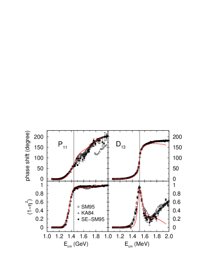
FIG. 1.: Phase shift and inelasticity in the partial waves $P_{11}$ and $D_{13}$. Data are taken from Ref. [2] (SM95) and [39, 1] (KA84). In addition, the single-energy analysis from [2] (SE-SM95) is shown. The vertical lines are drawn at $E=1440$ MeV ($P_{11}$) and $E=1520$ MeV ($D_{13}$) and correspond to the suggested values of the resonance masses as given in Ref. [9].

FIG. 2.: Contribution to the elastic $\pi N$ interaction.

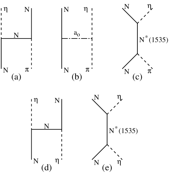
FIG. 3.: Additional contribution in coupling to the $\eta N$ channel.

FIG. 4.: Additional diagrams for coupling to the $\pi\Delta$ and $\sigma N$ channels.

FIG. 5.: The potential for the coupling to the $\rho N$ channel.

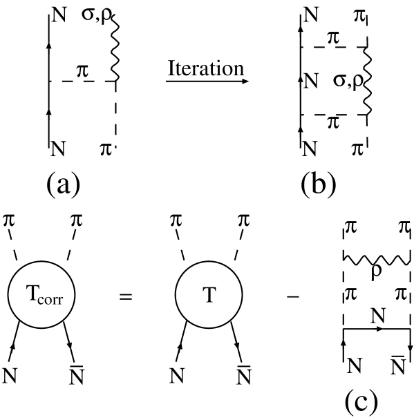
FIG. 6.: Double counting in the correlated $\pi\pi$ exchange arises from iteration of the $\pi$ exchange diagram (a), because that generates the box diagram (b), which is already included in the correlated $\pi\pi$ exchange (Fig. 2 (c)). In order to avoid double counting we remove the diagram (c) from the $N\bar{N}\to\pi\pi$ amplitudes.

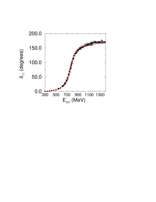
FIG. 7.: Phase shift in the partial wave $IJ=11$ of the $\pi\pi$ interaction. The solid line is the result of the self-energy calculation for the $\rho$ meson. Data is taken from Refs. [72, 73, 74].

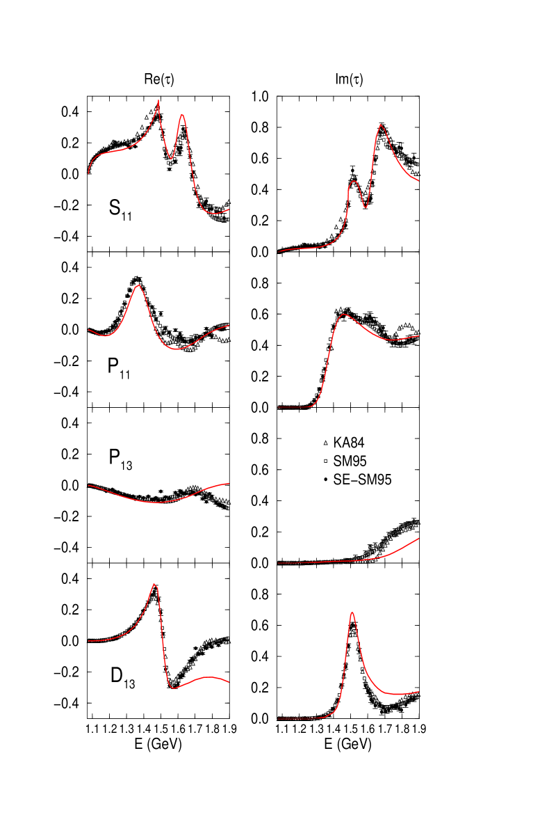
FIG. 8.: The $\pi N$ partial wave amplitudes for the isospin $I=\frac{1}{2}$. In addition, the analyses KA84 [39, 1] and SM95 [2], as well as the single-energy analysis SE-SM95 [2] are shown.

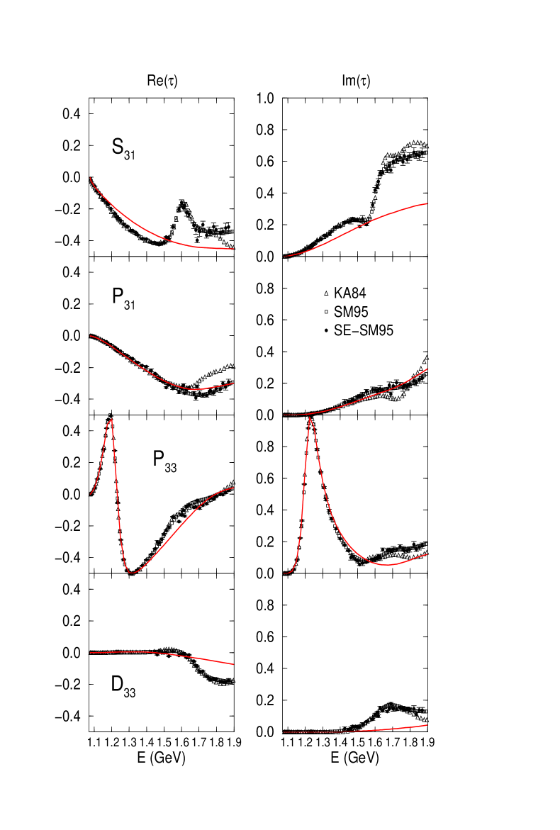
FIG. 9.: The partial wave amplitudes for $I=\frac{3}{2}$. The notation is the same as in Fig. 8.

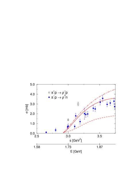
FIG. 10.: The transition cross section $\pi N\to\rho N$. The solid line shows the reaction $\pi^{-}p\to\rho^{0}n$, the dashed line the reaction $\pi^{-}p\to\rho^{-}p$ and the dot-dashed line the reaction $\pi^{+}p\to\rho^{+}p$. The experimental data are taken from Ref. [82].

FIG. 11.: Phase shift and inelasticity in the partial wave $P_{11}$. The curves are calculated using the full model (solid line), the channels $\pi N/\sigma N/\pi\Delta$ (dotted line), $\pi N/\pi\Delta$ (long dashed line), $\pi N/\sigma N$ (short dashed line), and the elastic model (dot-dashed line). The common parameters are the same in all five cases.

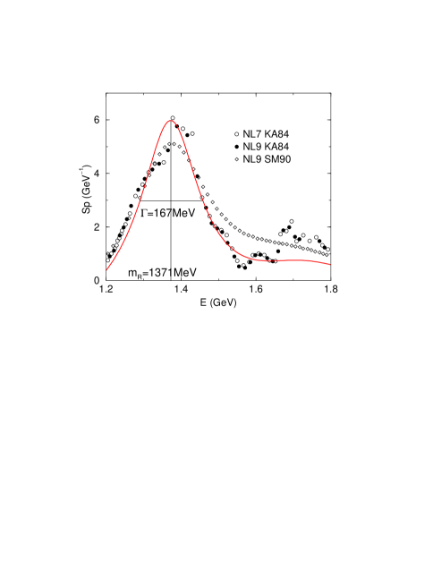
FIG. 12.: speed plot in the partial wave $P_{11}$. The symbols are showing speed plots from Ref. [36] (open circles) and Ref. [88] (full circles (KA84 [39, 1]) and diamonds (SM90 [37])).

FIG. 13.: The partial wave $P_{11}$ calculated with (dashed line) and without (solid line) $\pi$ exchange in the $\pi N\to\sigma N$ transition potential, using the same parameters.

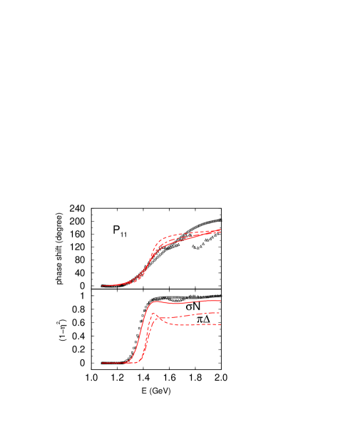
FIG. 14.: Results of the simplified model. The solid line was calculated using parameter set I of Table V, the dashed and dot-dashed curves are obtained using sets II and III, respectively. For the solid line only $\pi N$ and $\sigma N$ are coupled, whereas for the dashed and dot-dashed lines the only channels are $\pi N$ and $\pi\Delta$.

REFERENCES

- [1] R. Koch, Z. Phys. C 29, 597 (1985).
- [2] R.A. Arndt, I.I. Strakovsky, R.L. Workman, and M.M. Pavan, Phys. Rev. C 52, 2120 (1995).
- [3] R.A. Arndt, R.L. Workman, I.I. Strakovsky, and M.M. Pavan, LANL preprint nucl-th/9807087 (1998).
- [4] M. Batinic̀, I. laus, A. varc, and B.M.K. Nefkens, Phys. Rev. C 51, 2310 (1995).
- [5] T. Feuster and U. Mosel, Phys. Rev. C 59, 460 (1999).
- [6] T.P. Vrana, S.A. Dytman, and T.-S.H. Lee, LANL preprint nucl-th/9910012.
- [7] R.E. Cutkosky et al., Phys. Rev. D 20, 2804 and 2839 (1979).
- [8] D.M. Manley and E.M. Saleski, Phys. Rev. D 45, 4002 (1992).
- [9] C. Caso et al., Eur. Phys. J. C 3, 1 (1998).
- [10] B.S. Zou, G.X. Peng, H.C. Chiang, and P.N. Shen, LANL preprint hep-ph/9909204.
- [11] N. Isgur and G. Karl, Phys. Rev. D 18, 4187 (1978).
- [12] N. Isgur and G. Karl, Phys. Rev. D 19, 2653 (1979).
- [13] S. Capstick and N. Isgur, Phys. Rev. D 34, 2809 (1986).
- [14] L.Ya. Glozman and D.O. Riska, Phys. Rep. 268, 263 (1996).
- [15] R. Bijker, F. Iachello, and A. Leviatan, Phys. Rev. D 558, 2862 (1997).
- [16] K.F. Liu, S.J. Dong, T. Draper, D. Leinweber, J. Sloan, W. Wilox, and R.M. Woloshyn, Phys. Rev. D 59, 112001 (1999).
- [17] T. Yoshimoto, T. Sato, M. Arima, and T.-S. H. Lee, LANL preprint nucl-th/9908048.
- [18] N. Isgur, LANL preprint nucl-th/9908028.
- [19] L.Ya. Glozman, LANL preprint nucl-th/9909021.
- [20] Z. Li and F.E. Close, Phys. Rev. D 42, 2207 (1990).
- [21] Z. Li, V. Burkert, and Z. Li, Phys. Rev. D 46, 70 (1992).
- [22] S. Capstick, Phys. Rev. D 46, 1965 (1992).
- [23] S. Capstick and B.D. Keister, Phys. Rev. D 51, 3598 (1995).
- [24] F. Cardarelli, E. Pace, G. Salmgravee, and S. Simula, Phys. Lett. B397, 13 (1997).
- [25] Y.B. Dong, K. Shimizu, A. Faessler, and A.J. Buchmann, Phys. Rev. C 60, 035203 (1999).
- [26] S. Capstick and W. Roberts, Phys. Rev. D 47, 1994 (1993).
- [27] S. Capstick and W. Roberts, Phys. Rev. D 49, 4570 (1994).
- [28] Fl. Stancu and P. Stassart, Phys. Rev. D 41, 916 (1990).
- [29] Fl. Stancu and P. Stassart, Phys. Rev. D 39, 343 (1989).
- [30] P. Stassart, Phys. Rev. D 46, 2085 (1992).
- [31] R.E. Cutkosky and S. Wang, Phys. Rev. D 42, 235 (1990).
- [32] T. Barnes, RAL-94-056 and LANL preprint hep-ph/9406215.
- [33] K. Maltman and S. Godfrey, Nucl. Phys. A452 669 (1986).
- [34] Fl. Stancu, Phys. Rev. C 58 111501 (1998).
- [35] M. Genovese, J.-M. Richard, Fl. Stancu, and S. Pepin, Phys. Lett. B425 171 (1998).
- [36] G. Höhler and A. Schulte, Newsletter 7, 94 (1992).
- [37] R.A. Arndt, Z. Li, L.D. Roper, R.L. Workman, and J.M. Ford, Phys. Rev. D 43, 2131 (1991).
- [38] G. Höhler, Note on and resonances II. Against Breit-Wigner parameters – a pole-emic in Ref. [9].
- [39] G. Höhler, private communication.
- [40] B. Blankleider and G.E. Walker, Phys. Lett.B152, 291 (1985).
- [41] Y. Elmessiri and M.G. Fuda, Phys. Rev. C 57 2149 (1998).
- [42] A.B. Gridnev and N.G. Kozlenko, Eur. Phys. J. A 4, 187 (1999).
- [43] C.J. Joachain, Quantum Collision Theory (North-Holland Publihing Company, Amsterdam, 1975).
- [44] R. Machleidt, K. Holinde, and Ch. Elster, Phys. Rep. 149, 1 (1987).
- [45] A.M. Badalyan et al., Phys. Rep. 82, 31 (1982).
- [46] J. Weinstein and N. Isgur, Phys. Rev. D 41, 2236 (1990).
- [47] G. Janßen, B.C. Pearce, K. Holinde, and J. Speth, Phys. Rev. D 52, 2690 (1995).
- [48] P.B. Siegel and W. Weise, Phys. Rev. C 38, 2221 (1988).
- [49] A. Müller-Groeling, K. Holinde, and J. Speth, Nucl. Phys. A513, 557 (1990).
- [50] C. Schütz, J. Haidenbauer, J.W. Durso, and J. Speth, Phys. Rev. C 57, 1464 (1998).
- [51] R. Böckmann, C. Hanhart, O. Krehl, S. Krewald, and J. Speth, Phys. Rev. C 60, 055212 (1999).
- [52] B.C. Pearce and B.K. Jennings, Nucl. Phys. A528, 655 (1991).
- [53] C. Lee, S.N. Yang, and T.-S. H. Lee, J. Phys. G 17, (1991).
- [54] F. Gross and Y. Surya, Phys. Rev. C 47, 703 (1993).
- [55] C.T. Hung, S.N. Yang, and T.-S. H. Lee, J. Phys. G 20, 1531 (1994).
- [56] P.F.A. Goudsmit, H.J. Leisi, E. Matsinos, B.L. Birbrair, and A.B. Gridnev, Nucl. Phys. A575, 673 (1994).
- [57] V. Pascalutsa and J.A. Tjon, Nucl. Phys. A631, 534c (1998).
- [58] A.D. Lahiff and I.R. Afnan, LANL preprint nucl-th/9903058.
- [59] R. Buettgen, K. Holinde, A. Mueller-Groeling, J. Speth and P. Wyborny, Nucl. Phys. A506, 586 (1990).
- [60] J. Wess and B. Zumino, Phys. Rev. 163, 1727 (1967). 2671 (1994).
- [61] O. Krehl, C. Hanhart, S. Krewald, and J. Speth, Phys. Rev. C 60, 055206 (1999).
- [62] C. Schütz, K. Holinde, J. Speth, B.C. Pearce und J.W. Durso, Phys. Rev. C 51, 1374 (1995).
- [63] K. Erkelenz, Phys. Rep. 5, 191 (1974).
- [64] J.H. Hetherington and L.H. Schick, Phys. Rev. B 137, 935 (1965).
- [65] R. Aaron and R.D. Amado, Phys. Rev. 150, 857 (1966).
- [66] R.T. Cahill and I.H. Sloan, Nucl. Phys. A165, 161 (1971).
- [67] M. Jacob and G.C. Wick, Ann. Phys. (N.Y.) 7, 404 (1959).
- [68] C. Schütz, J.W. Durso, K. Holinde, and J. Speth, Phys. Rev. C 49,
- [69] G. Höhler, in Pion-Nucleon Scattering, edited by H. Schopper, Landolt-Börnstein, New Series, Group I, Vol. 9b, Pt. 2 (Springer-Verlag, New York, 1983).
- [70] I.R. Afnan, Acta Phys. Polon. B 29, 2397 (1998).
- [71] J.A. Elsey and I.R. Afnan, Phys. Rev. D 40, 2353 (1989).
- [72] W. Ochs, Thesis, unpublished (München, 1973).
- [73] C.D. Froggatt and J.L. Petersen, Nucl. Phys. B129, 89 (1977).
- [74] B. Hyams et al., Nucl. Phys. B100, 205 (1975).
- [75] G. Janßen, K. Holinde, and J. Speth, Phys. Rev. C 54, 2218 (1996).
- [76] C. Schütz, Berichte des Forschungszentrums Jülich, Nr. 3130 (1995).
- [77] G.E. Brown and W. Weise, Phys. Rep. 22, 279 (1975).
- [78] J.W. Durso, A.D. Jackson and B.J. Verwest, Nucl. Phys. A345, 471 (1980).
- [79] O. Krehl and J. Speth, Nucl. Phys. A623, 162c (1997).
- [80] K. Nakayama, A. Szczurek, C. Hanhart, J. Haidenbauer, and J. Speth, Phys. Rev. C 57, 1580 (1998).
- [81] J.W. Durso, Phys. Lett. B 184, 348 (1987).
- [82] Handbook of Physics, Landolt–Börnstein, edited by H. Schopper (Springer, Berlin, 1987), Vol. 12/a.
- [83] R. Aaron, R.D. Amado und J.E. Young., Phys. Rev. 174, 2022 (1968).
- [84] R. Aaron, D.C. Teplitz, R.D. Amado und J.E. Young, Phys. Rev. 187, 2047 (1969).
- [85] O. Krehl, C. Hanhart, S. Krewald, and J. Speth, in preparation.
- [86] M.L. Goldberger and K.M. Watson, Collision Theory (John Wiley and Sons, New York, 1964).
- [87] A. Bohm, Quantum Mechanics: Foundations and Applications (Springer–Verlag, New York, 1993).
- [88] G. Höhler, N Newsletter 9, 1 (1993).
- [89] R.J. McLeod and I.R. Afnan, Phys. Rev. C 32, 222 (1985).
- [90] I.R. Afnan and A.T. Stelbovics, Phys. Rev. C 23, 1384 (1981).
- [91] W.R. Frazer and J.R. Fulco, Phys. Rev. 117, 1609 (1960).
- [92] F. Gross, Relativistic Quantum Mechanics and Field Theory (John Wiley & Sons, New York, 1993).
- [93] S.S. Schweber, An Introduction to relativistic Quantum Field Theory (Harper and Row, New York, 1962).