SU(3) realization of the rigid asymmetric rotor within the IBM

Abstract

It is shown that the spectrum of the asymmetric rotor can be realized quantum mechanically in terms of a system of interacting bosons. This is achieved in the SU(3) limit of the interacting boson model by considering higher-order interactions between the bosons. The spectrum corresponds to that of a rigid asymmetric rotor in the limit of infinite boson number.

It is well known that the dynamical symmetry limits of the simplest version of the interacting boson model (IBM) [1, 2], IBM-1, correspond to particular types of collective nuclear spectra. A Hamiltonian with U(5) dynamical symmetry [3] has the spectrum of an anharmonic vibrator, the SU(3) Hamiltonian [4] has the rotation-vibration spectrum of vibrations around an axially symmetric shape and the SO(6) Hamiltonian [5] yields the spectrum of a $\gamma$-unstable nucleus [6]. There exists another interesting type of spectrum frequently used to interpret nuclear collective excitations which corresponds to the rotation of a rigid asymmetric top [7] and which, up to now, has found no realization in the context of the IBM-1. The purpose of this letter is to extend the IBM-1 towards high-order terms such that a realization of the rigid non-axial rotor of Davydov and Filippov becomes possible. A pure group-theoretical approach is used that allows to establish the connection between algebraic and geometric Hamiltonians not only from the comparison of their spectra but also from the underlying group properties.

Let us first recall some of the aspects that have enabled a geometric understanding of the IBM. The relation between the Bohr-Mottelson collective model [8] and the IBM has been established [9, 10] on the basis of an intrinsic (or coherent) state for the IBM. Via this coherent-state formalism, a potential energy surface $E(\beta,\gamma)$ in the quadrupole deformation variables $\beta$ and $\gamma$ can be derived for any IBM Hamiltonian and the equilibrium deformation parameters $\beta_{0}$ and $\gamma_{0}$ are then found by minimizing $E(\beta,\gamma)$. It is by now well established that a one- and two-body IBM-1 Hamiltonian can give rise only to axially symmetric equilibrium shapes ($\gamma_{0}=0^{\rm o}\;{\rm or}\;60^{\rm o}$) [9, 10] and that a triaxial minimum in the potential energy surface requires at least three-body interactions [11].

Since the relationship between $\gamma$-unstable model and rigid triaxial rotor was always an open question, Otsuka et al. [12, 13] investigated in detail the SO(6) solutions of one- and two-body IBM-1 Hamiltonian. They found out that the triaxial intrinsic state with $\gamma_{0}=30^{\rm o}$ produces after the angular momentum projection the exact SO(6) eigenfunctions for small numbers of bosons $N$. Thus they conclude that for finite boson systems triaxiality reduces to $\gamma$-unstability.

If three-body terms are included in the IBM-1 Hamiltonian a triaxial minimum of the nuclear potential energy surface can be found and numerous studies of the corresponding spectra have been performed [11, 14, 15, 16, 17, 18, 19]. However, the existence of a minimum in the potential energy surface at $0^{\rm o}<\gamma<60^{\rm o}$ is not a sufficient condition for a rigid triaxial shape since this minimum can be shallow indicating a $\gamma$-soft nucleus. The interest in higher-order terms in IBM-1 has been renewed recently by the challenging problem of anharmonicities of double-phonon excitations in well-deformed nuclei [20, 21]. Although their microscopic origin is not clear at the moment, the occurrence of higher-order interactions can be understood qualitatively as a result of the projection of two-body interactions in the proton-neutron IBM [22] onto the symmetric IBM-1 subspace. For example, it is well known that triaxial deformation arises within the SU^∗(3) dynamical symmetry limit [23] of the proton-neutron IBM without any recourse to interactions of order higher than two.

Nuclear collective states are treated in IBM-1 in terms of $N$ bosons of two types: monopole ($l^{\pi}=0^{+}$) $s$ bosons and quadrupole ($l^{\pi}=2^{+}$) $d$ bosons [2]. For a given nucleus, $N$ is the half number of valence nucleons (or holes) and is thus fixed. Analytical solutions can be constructed for particular forms of the Hamiltonian which correspond to one of the three possible reduction chains of the dynamical group of the model U(6):

$${\begin{array}[]{ccl}&&\mbox{U(5)}\supset\mbox{SO(5)}\supset\mbox{SO(3)}\\ &\nearrow\\ \mbox{U(6)}&\rightarrow&\mbox{SU(3)}\supset\mbox{SO(3)}\\ &\searrow&\\ &&\mbox{SO(6)}\supset\mbox{SO(5)}\supset\mbox{SO(3)}\\ \end{array}}.$$ (1)

The SU(3) dynamical symmetry Hamiltonian corresponds to a rotation-vibration spectrum of a vibrations around an axially symmetric shape which in the limit $N\to\infty$ goes over into the spectrum of a rigid axial rotor [9]. The two other reduction chains in (1) contain the SO(5) group whose Casimir invariant exactly corresponds to $\gamma$-independent potential of Wilets and Jean [6] and is responsible for $\gamma$-soft character of the spectrum [24, 25].

To obtain a rigid (at least for $N\to\infty$) triaxial rotor the starting point is the SU(3) limit of the IBM-1 with higher-order terms in the Hamiltonian. This approach is inspired by Elliott’s SU(3) model [26, 27] where the rotor dynamics is well established for SU(3) irreducible representations (irreps) with large dimensions.

Following Ref. [28], we consider the most general SU(3) dynamical symmetry Hamiltonian constructed from the second, third and fourth order invariant operators of the SU(3) $\supset$ SO(3) integrity basis [29]:

$$H_{\rm IBM}=H_{0}+aC_{2}+bC_{2}^{2}+cC_{3}+d\Omega+e\Lambda+fL^{2}+gL^{4}+hC_{2}L^{2}\;.$$ (2)

Here the following notation is used:

$$\begin{array}[]{r@{\ }l}C_{2}&\equiv C_{2}[\mbox{SU(3)}]=2Q^{2}+\frac{3}{4}L^{2}\;,\end{array}$$ (10)

$$\begin{array}[]{r@{\ }l}C_{3}&\equiv C_{3}[\mbox{SU(3)}]=-\frac{4}{9}\sqrt{35}[Q\times Q\times Q]^{(0)}_{0}-\frac{\sqrt{15}}{2}[L\times Q\times L]^{(0)}_{0}\;,\\ \end{array}$$

$$\begin{array}[]{r@{\ }l}\Omega&=-3\sqrt{\frac{5}{2}}[L\times Q\times L]^{(0)}_{0}\;,\\ \end{array}$$

$$\begin{array}[]{r@{\ }l}\Lambda&=\left[L\times Q\times Q\times L\right]^{(0)}_{0}\;,\\ \end{array}$$

where

$$L_{q}=\sqrt{10}[d^{+}\,{\times}\,\tilde{d}]^{(1)}_{q}\;,$$ (11)

$$Q_{q}=[d^{+}\,{\times}\,s+s^{+}\,{\times}\,\tilde{d}]^{(2)}_{q}-\frac{\sqrt{7}}{2}[d^{+}\,{\times}\,\tilde{d}]^{(2)}_{q}\;,$$ (12)

are SU(3) generators, satisfying the standard commutation relations,

$$\begin{array}[]{l}[L_{q},L_{q^{\prime}}]=-\sqrt{2}(1q1q^{\prime}|1q+q^{\prime})L_{q+q^{\prime}}\;,\\[0.0pt] [L_{q},Q_{q^{\prime}}]=-\sqrt{6}(1q2q^{\prime}|2q+q^{\prime})Q_{q+q^{\prime}}\;,\\[0.0pt] [Q_{q},Q_{q^{\prime}}]=\frac{3}{4}\sqrt{\frac{5}{2}}(2q2q^{\prime}|1q+q^{\prime})L_{q+q^{\prime}}\;.\end{array}$$ (13)

In the context of the shell model, an SU(3) Hamiltonian of the type (2) has been considered by a number of authors [30, 31, 32, 33, 34, 35]. Specifically, it was established [31] that the rotor Hamiltonian can be constructed from $L^{2}$ and the SU(3) invariants $\Omega$ and $\Lambda$. This follows from the asymptotic properties of these SU(3) invariants whose spectra do correspond to rigid triaxial rotor for SU(3) irrep labels $\lambda,\mu\to\infty$. In addition, a relation between ($\lambda,\mu$) and the collective variables ($\beta,\gamma$) characterizing the shape of the rotor can be derived [33]. In contrast, all attempts so far to construct a rigid rotor in the SU(3) dynamical symmetry limit of the IBM-1, even if including higher-order terms, are restricted to axial shapes [28].

A noteworthy difference should be pointed out between the SU(3) realizations in the shell model and the IBM and concerns the irreps that occur lowest in energy. In the shell model the ground-state irrep is dictated by the leading shell-model configuration. For example, it is (8,4) for ²⁴Mg and (30,8) for ¹⁶⁸Er [26, 31]. In the IBM the lowest representation is determined by the Hamiltonian. One can show that for an SU(3) Hamiltonian with two- and three-body interactions it is either $(2N,0)$ or $(0,N)$, which corresponds to axially symmetric nucleus. The essential point that is exploited here is that this choice of the lowest SU(3) irrep becomes more general for the IBM-1 Hamiltonian with up to four-body terms.

One can show that with the linear combination

$$F=aC_{2}+bC_{2}^{2}\;,$$ (14)

any given irrep $(\lambda_{0},\mu_{0})$ that occurs for a system of $s$ and $d$ bosons can, in principle, be brought lowest in energy. The proof is as follows. The eigenvalue of the second-order SU(3) Casimir invariant is

$$g_{2}(\lambda,\mu)=\lambda^{2}+\mu^{2}+\lambda\mu+3\lambda+3\mu\;.$$ (15)

Within a given U(6) irrep $[N]$ the following SU(3) $(\lambda,\mu)$ values are admissible [26]:

$$\begin{array}[]{ll}(\lambda,\mu)=&(2N,0),\;(2N-4,2),\;\ldots\;(2,N-1)\quad{\rm or}\quad(0,N)\;,\\[0.0pt] &(2N-6,0),\;(2N-10,2),\;\ldots\;(2,N-4)\quad{\rm}\quad(0,N-3)\;,\\[0.0pt] &\ldots\\ &(4,0),\;(0,2)\quad{\rm for}\quad N({\rm mod}3)=2\;,\\[0.0pt] &(2,0)\quad{\rm for}\quad N({\rm mod}3)=1\;,\\[0.0pt] &(0,0)\quad{\rm for}\quad N({\rm mod}3)=0\;.\\[0.0pt] \end{array}$$ (16)

For the first row in this equation (which corresponds to the largest values of Casimir invariants) one has the relation

$$2N=\lambda+2\mu\;,$$ (17)

and consequently $g_{2}(\lambda,\mu)\equiv g_{N}(\lambda)$. The eigenvalues of (14) are thus given by

$$F_{N}(\lambda)=ag_{N}(\lambda)+bg_{N}^{2}(\lambda)\;.$$ (18)

Minimization of this function with respect to $\lambda$ gives the following condition for the irrep $(\lambda_{0},\mu_{0})$ to be lowest in energy:

$$\frac{a}{b}=-2g(\lambda_{0},\mu_{0})\;.$$ (19)

It is worth mentioning that one fails to obtain a similar minimization condition with just the second- and third-order SU(3) Casimir invariants.

Once $(\lambda_{0},\mu_{0})$ is fixed, the constant part of the Hamiltonian (2) takes the form

$$\tilde{H}_{0}=H_{0}-bg_{2}^{2}(\lambda_{0},\mu_{0})+cg_{3}(\lambda_{0},\mu_{0})\;,$$ (20)

where $g_{3}(\lambda,\mu)$ is the expectation value of $C_{3}$[SU(3)]

$$g_{3}(\lambda,\mu)=\frac{1}{9}(\lambda-\mu)(2\lambda+\mu+3)(\lambda+2\mu+3)\;,$$ (21)

and the Hamiltonian (2) can be rewritten as

$$H_{\rm IBM}=\tilde{H}_{0}+d\Omega+e\Lambda+\tilde{f}L^{2}+gL^{4}\;,$$ (22)

where $\tilde{f}=f+hg_{2}(\lambda_{0},\mu_{0})$.

To see the relation between this Hamiltonian and that of the rotor, we rewrite (22) further as

$$H_{\rm IBM}=\tilde{H}_{0}+d(L_{i}Q_{ij}L_{j})+e(L_{i}Q_{ik}Q_{kj}L_{j})+\tilde{f}L^{2}+gL^{4}\;,$$ (23)

where $Q_{ij}$ are cartesian components of the quadrupole tensor (12). This operator has the same functional form as the rigid rotor Hamiltonian

$$H_{\rm rotor}=A_{i}{\rm L}_{i}^{2}=(L_{i}M_{ij}L_{j})\;,$$ (24)

where ${\rm L}_{i}$ ($L_{i}$) are the components of the angular momentum $L$ in the intrinsic (laboratory) frame, $M_{ij}$ is a moments of inertia tensor with the constant components. The parameters of inertia $A_{i}$ are related to the principal moments of inertia ${\cal I}_{i}$ as

$$A_{i}=\frac{\hbar^{2}}{2{\cal I}_{i}}\;.$$ (25)

The rotor moments of inertia tensor is connected with the SU(3) quadrupole tensor components through

$$M_{ij}=[\tilde{f}+gL(L+1)]\delta_{ij}+dQ_{ij}+eQ_{ik}Q_{kj}\;.$$ (26)

Note that, in general, the components of the quadrupole tensor $Q_{ij}$ fluctuate around their average values. When these fluctuations are negligible, the spectrum of the IBM-1 Hamiltonian (23) is close to the spectrum of rigid asymmetric rotor with corresponding moments of inertia.

The analogy between the rigid rotor and SU(3) dynamical symmetry Hamiltonians can be studied from a group-theoretical point of view. The dynamical group of the quantum rotor [36] is the semidirect product T₅ $\wedge$ SO(3) where T₅ is generated by the five components of the collective quadrupole operator $\overline{Q}$. The operators $\overline{Q}$ and $L$ satisfy the commutation relations

$$\begin{array}[]{l}[L_{q},L_{q^{\prime}}]=-\sqrt{2}(1q1q^{\prime}|1q+q^{\prime})L_{q+q^{\prime}}\;,\\[0.0pt] [L_{q},\overline{Q}_{q^{\prime}}]=-\sqrt{6}(1q2q^{\prime}|2q+q^{\prime})\overline{Q}_{q+q^{\prime}}\;,\\[0.0pt] [\overline{Q}_{q},\overline{Q}_{q^{\prime}}]=0\;,\end{array}$$ (27)

which define the rotor Lie algebra t₅ $\oplus$ so(3). The only difference between (13) and (27) is in the last commutator.

The replacement $Q\to Q/\sqrt{C_{2}}$ in the su(3) algebra leads to $[Q_{q},Q_{q^{\prime}}]\to 0$ for $\lambda,\mu\gg L$. Thus for large $\lambda$ and $\mu$ the su(3) algebra contracts to the rigid rotor algebra t₅ $\oplus$ so(3). The irreps of t₅ $\oplus$ so(3) are characterized by the $\beta$ and $\gamma$ shape variables which can be related to SU(3) irrep labels $\lambda$ and $\mu$ as in Ref. [33]:

$$\begin{array}[]{l}\kappa\beta\cos{\gamma}=\frac{1}{3}(2\lambda+\mu+3)\;,\\ \kappa\beta\sin{\gamma}=\frac{1}{\sqrt{3}}(\mu+1)\;,\\ \end{array}$$ (28)

where $\kappa$ has to be determined from parameterization

$$\overline{Q}_{q}=\kappa\beta[\delta_{q0}\cos{\gamma}+\frac{1}{\sqrt{2}}(\delta_{q2}+\delta_{q,-2})\sin{\gamma}]\;,$$ (29)

with $\beta\geq 0$ and $0^{\rm o}\leq\gamma\leq 60^{\rm o}$.

The difference between the shell model SU(3) realization and the SU(3) dynamical symmetry limit of the IBM can be visualized on a $(\beta,\gamma)$ plot which gives the relation between $(\beta,\gamma)$ and the SU(3) labels $(\lambda,\mu)$ [33] (see Figure 1). The SU(3) irreps valid for the IBM (marked by circles) are only a subset of those which are allowed in the shell model in accordance with the Pauli principle (e.g., Fig. 2 in Ref. [35]).

From a group-theoretical point of view, the difference is seen from the following considerations. The invariant symmetry group of the asymmetric rotor is the point symmetry group D₂, whose irreps can be classified as $A_{1}$, $B_{1}$, $B_{2}$ and $B_{3}$. In the contraction limit, the $(\lambda,\mu)$ irrep of SU(3) reduces to one of the D₂ irreps according to the even or odd values of $\lambda$ or $\mu$. Since the IBM only allows even $\lambda$ and $\mu$, only totally symmetric $A_{1}$ levels of the asymmetric rotor can be represented. These are also the asymmetric rotor levels, which should be considered [7] in connection with nuclear spectra.

As an example, in Figure 2 the spectrum of the Hamiltonian (2) is shown with the parameters $a=-72$ keV, $b=0.1$ keV, $d=0.1$ keV, $f=25$ keV, $c=e=g=h=0$ and $H_{0}=12960$ keV for the two lowest SU(3) irreps $(10,10)$ and $(14,8)$ of an $N=15$ boson system and compared with the spectrum of an asymmetric rotor of highest asymmetry ($\gamma=30^{\rm o}$). The matrices of the operators $\Omega$ and $\Lambda$ in the Elliott’s basis can be found in Refs. [28, 37]. The SU(3) spectrum consists of $(\lambda,\mu)$-multiplets within which the levels are arranged in bands characterized by Elliott’s quantum number $K$ where for even $\lambda$ and $\mu$

$$\begin{array}[]{l}K={\rm min}\{\lambda,\mu\},{\rm min}\{\lambda,\mu\}-2,\;\ldots\;,2\;{\rm or}\;0\;,\\ L=K,K+1,\;\ldots\;,{\rm max}\{\lambda,\mu\}\quad{\rm for}\;K\neq 0\;,\\ L=0,2,\;\ldots\;,{\rm max}\{\lambda,\mu\}\quad{\rm for}\;K=0\;.\\ \end{array}$$ (30)

The spectrum of a triaxial rotor consists of a ground-state band with $L=0,2,4,\;\ldots$ and an infinite number of the so-called abnormal bands: $L=2,3,4,5,\;\ldots$ (1st abnormal band), $L=4,5,6,7,\;\ldots$ (2nd abnormal band), and so on. Contrary to the axially symmetric case, the projection of the angular momentum $L$ on the intrinsic $z$-axis no longer is a good quantum number. Also, the spectrum contains $L/2+1$ states for $L$ even and $(L-1)/2$ states for $L$ odd. It is seen that the low-energy spectrum corresponding to $(10,10)$ irrep is remarkably close to the spectrum of the asymmetric rotor. The resemblance includes the prominent even-odd staggering in the first abnormal band which is a perfect signature to distinguish axial, rigid or soft triaxial rotors (see, e.g. Refs. [17, 19]). Eventual differences between the triaxial rotor and the SU(3) calculation are caused by the finite number of allowed $L$-values for each $K$ in a given $(\lambda,\mu)$ irrep.

Although the above considerations were limited to the SU(3) dynamical symmetry, we would like to stress that this is not the only possible realization of rigid triaxiality in the IBM-1. As has been demonstrated recently [21], a rotational spectrum can be generated by only quadratic $[Q^{0}\times Q^{0}]^{(0)}$ and cubic $[Q^{0}\times Q^{0}\times Q^{0}]^{(0)}$ SO(6) invariants where

$$Q^{0}_{q}=[d^{+}\,{\times}\,s+s^{+}\,{\times}\,\tilde{d}]^{(2)}_{q}$$ (31)

is an SO(6) generator. This can be understood from a group-theoretical point of view. In the limit $[Q^{0}_{q},Q^{0}_{q^{\prime}}]\to 0$ the so(6) algebra contracts to the rigid rotor algebra t₅ $\oplus$ so(3) and a rigid rotor realization with SO(6) dynamical symmetry is obtained in IBM-1.

Inspired by this result, it would be of interest to inspect the Hamiltonian of the type (2)

$$H_{\rm IBM}=H_{0}+\alpha(L_{i}Q^{\chi}_{ij}L_{j})+\eta(L_{i}Q^{\chi}_{ik}Q^{\chi}_{kj}L_{j})+\zeta L^{2}+\xi L^{4}\;,$$ (32)

where $Q^{\chi}$ is a general quadrupole operator

$$Q^{\chi}_{q}=[d^{+}\,{\times}\,s+s^{+}\,{\times}\,\tilde{d}]^{(2)}_{q}+\chi[d^{+}\,{\times}\,\tilde{d}]^{(2)}_{q}\;.$$ (33)

One expects that, provided the commutation relations for $L$ and $Q^{\chi}$ are close to those for the rotor (27), the spectrum of the Hamiltonian (32) should resemble that of the rigid rotor.

In summary, an IBM-1 realization of the rigid rotor has been suggested. Although the example has been restricted to the SU(3) dynamical symmetry, any Hamiltonian of a similar type constructed with general quadrupole operator and with the angular momentum operator produces a rigid rotor spectrum under the condition of appropriate commutation relations. The required and sufficient condition to obtain the rotor dynamics is the contraction of the dynamical algebra of the Hamiltonian to the rigid rotor algebra t₅ $\oplus$ so(3).

We gratefully acknowledge discussions with P. von Brentano, F. Iachello, D. F. Kusnezov, S. Kuyucak, A. Leviatan, N. Pietralla, A. A. Seregin and A. M. Shirokov. N.A.S. and P.V.I. thank the Institute for Nuclear Theory at the University of Washington for its hospitality and support. Yu.F.S. thanks GANIL for its hospitality The work is partly supported by Russian Foundation of Basic Research (grant 99-01-0163).

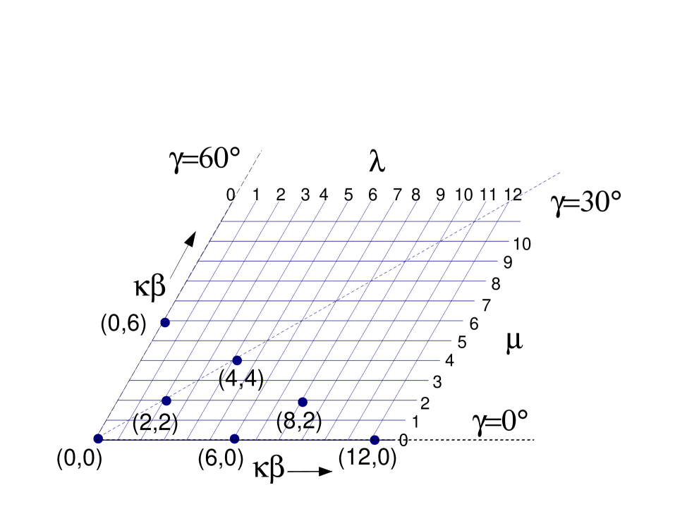
FIG. 1.: Relation between the collective rotor parameters $(\beta,\gamma)$ and the SU(3) irrep labels $(\lambda,\mu)$. The circles indicate the irreps valid for the IBM with $N=6$ bosons.

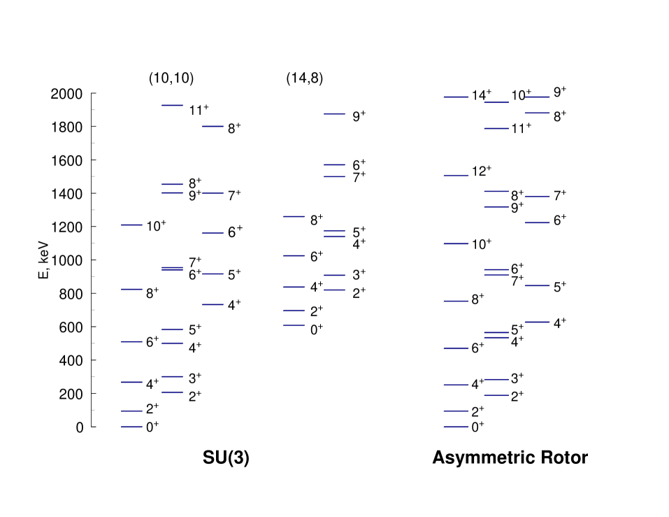
FIG. 2.: Left: a typical spectrum of the SU(3) dynamical symmetry Hamiltonian (2) with the set of parameters $a=-72$ keV, $b=0.1$ keV, $d=0.1$ keV, $f=25$ keV, $c=e=g=h=0$ and $H_{0}=12960$ keV for $N=15$ bosons. The two lowest SU(3) irreps $(10,10)$ and $(14,8)$ are shown. Right: the asymmetric rotor spectrum for $\gamma=30^{\rm o}$.

REFERENCES

- [1] A. Arima and F. Iachello, Phys. Rev. Lett. 35, 1069 (1975).
- [2] F. Iachello and A. Arima, The Interacting Boson Model (Cambridge, 1987).
- [3] A. Arima and F. Iachello, Ann. Phys. (N.Y.) 99, 253 (1976).
- [4] A. Arima and F. Iachello, Ann. Phys. (N.Y.) 111, 201 (1976).
- [5] A. Arima and F. Iachello, Ann. Phys. (N.Y.) 123, 468 (1979).
- [6] J. Wilets and M. Jean, Phys. Rev. 102, 788 (1956).
- [7] A. S. Davydov and G. F. Filippov, Nucl. Phys. 8, 237 (1958).
- [8] A. Bohr and B. R. Mottelson, Nuclear Structure II (Benjamin, New York, 1975).
- [9] J. N. Ginocchio and M. W. Kirson, Phys. Rev. Lett. 44, 1744 (1980).
- [10] A. E. L. Dieperink, O. Scholten, and F. Iachello, Phys. Rev. Lett. 44, 1747 (1980).
- [11] P. Van Isacker and Jin-Quan Chen, Phys. Rev. C 24, 684 (1981).
- [12] T. Otsuka and M. Sugita, Phys. Rev. Lett. 59, 1541 (1987).
- [13] M. Sugita, T. Otsuka, and A. Gelberg, Nucl. Phys. A 493, 350 (1989).
- [14] K. Heyde, P. Van Isacker, M. Waroquier, and J. Moreau, Phys. Rev. C 29, 1420 (1984).
- [15] R. F. Casten, P. von Brentano, K. Heyde, P. Van Isacker, and J. Jolie, Nucl. Phys. A 439, 289 (1985).
- [16] A. Leviatan and B. Shao, Phys. Lett. B 243, 313 (1990).
- [17] N. V. Zamfir and R. F. Casten, Phys. Lett. B 260, 265 (1991).
- [18] Liao Ji-zhi and Wang Huang-sheng, Phys. Rev. C 49, 2465 (1994).
- [19] Liao Ji-zhi, Phys. Rev. C 51, 141 (1995).
- [20] J. E. García-Ramos, C. E. Alonso, J. M. Arias, and P. Van Isacker, unpublished.
- [21] P. Van Isacker, Phys. Rev. Lett. 83, (1999).
- [22] A. Arima, T. Otsuka, F. Iachello, and I. Talmi, Phys. Lett. B 66, 205 (1977).
- [23] A. E. L. Dieperink and R. Bijker, Phys. Lett. B 116, 77 (1982).
- [24] D. R. Bes, Nucl. Phys. 10, 373 (1958).
- [25] A. Leviatan, A. Novoselsky, and I. Talmi, Phys. Lett. B 172, 144 (1986).
- [26] J. P. Elliott, Proc. Roy. Soc. A 245, 128, 562 (1958).
- [27] J. P. Elliott and M. Harvey, Proc. Roy. Soc. A 272, 557 (1963).
- [28] G. Vanden Berghe, H. E. De Meyer, and P. Van Isacker, Phys. Rev. C 32, 1049 (1985).
- [29] B. R. Judd, W. Miller Jr., J. Patera, and P. Winternitz, J. Math. Phys. 15, 1787 (1974).
- [30] J. P. Draayer and G. Rosensteel, Nucl. Phys. A 439, 61 (1985).
- [31] Y. Leschber and J. P. Draayer, Phys. Rev. C 33, 749 (1986).
- [32] J. Carvalho, R. Le Blanc, M. Vassanji, D. J. Rowe, and J. M. McGrory, Nucl. Phys. A 452, 240 (1986).
- [33] O. Castaños, J. P. Draayer, and Y. Leschber, Z. Phys. A 329, 33 (1988).
- [34] P. Rochford and D. J. Rowe, Phys. Lett. B 210, 5 (1988).
- [35] C. Bahri, J. Escher, and J. P. Draayer, Nucl. Phys. A 592, 171 (1995).
- [36] H. Ui, Progr. Theor. Phys. 44, 153 (1970).
- [37] G. F. Filippov, V. I. Ovcharenko, and Yu. F. Smirnov, Microscopic theory of collective nuclear excitations (Kiev, 1981).