Damping of IVGDR - Fermi-liquid or Fermi-gas ?

Recently the experimental observation of temperature dependence of IVGDR has raised much interest in theoretical investigations. The hope is that the temperature dependence gives insight into the character of bulk nuclear matter. In analogy to zero sound damping the nuclear matter is thought to be described as a Fermi liquid. However there is not paid much attention to the fact that a Fermi liquid leads to different predictions as the Fermi gas. In Ref.²⁾ the calculation was performed within a Fermi gas model and later corrected in an errata. The latter one was claimed to be performed as a Fermi liquid with an additional contribution from the quasiparticles to the Fermi gas. We will show that the quasiparticle part alone leads to the Landau damping of zero sound³⁾⁴⁾.

With the experimental data at hand we have the possibility to check which behavior describes the temperature dependence more appropriate.

In this letter we shortly sketch the derivation of the damping of a collective mode within a Fermi gas and a Fermi liquid model. We will show that we get the latter one from the Fermi gas model with an additional contribution from the quasiparticles.

We start with the Fermi gas where the dispersion relation between momentum and energy is given by $\epsilon=p^{2}/2m$ and will show later what has to be changed for a Fermi liquid where $\epsilon$ is a solution of the quasiparticle dispersion relation. We will see that the contributions from the quasiparticles alone leads to the Landau formula of zero sound damping³⁾⁴⁾

$$\gamma\propto\left[1+\left({\Omega\over 2\pi T}\right)^{2}\right].$$ (1)

Our considerations will start conveniently from the Levinson equation for the reduced density matrix $f$ which is valid at short time processes compared to inverse Fermi energy $\hbar/\epsilon_{f}$:

$$\partial_{t}f_{1}(t)={2g\over\hbar^{2}}\int\limits_{0}^{\infty}d\tau\int{dp_{2}dp_{3}dp_{4}\over(2\pi\hbar)^{6}}|T|^{2}$$

$$\times\cos{\left(\int\limits_{t}^{t-\tau}\Delta\epsilon(\tau)d\tau/\hbar\right)}\delta(\Delta p)\left({\bar{f}_{1}}{\bar{f}_{2}}f_{3}f_{4}-f_{1}f_{2}{\bar{f}_{3}}{\bar{f}_{4}}\right)_{t-\tau}$$

(2)

where ${\bar{f}}=1-f$, $\Delta p=p_{1}+p_{2}-p_{3}-p_{4}$ etc., g is the spin-isospin degeneracy and the transition probability is given by the scattering $T$-matrix. In case that the quasiparticle energies $\epsilon(t)$ become time independent like in the Fermi gas model, the integral in the $cos$ function reduces to the familiar expression $\Delta\epsilon\tau$. We linearize this collision integral with respect to an external disturbance according to

$$f=n+\delta f$$ (3)

where n is the equilibrium distribution. Clearly two contributions have to be distinguished, the one from the quasiparticle energy and the one from occupation factors¹⁾. First we concentrate on the Fermi gas model where we have only the contribution of the occupation factors and will later add the contribution of the quasiparticle energies for Fermi liquid model. We obtain after Fourier transform of the time

$$-i\Omega\delta f_{1} = \Big{\langle}\frac{\hbar}{2}\left[\delta_{+}(\Delta\epsilon+\Omega)+\delta_{-}(\Delta\epsilon-\Omega)\right]$$ (4)

$$\times \left(\delta F_{1}+\delta F_{2}-\delta F_{3}-\delta F_{4}\right)(\Omega)\Big{\rangle}.$$

Here we use the abbreviation

$$\langle...\rangle = {2g\over\hbar^{2}}\int{dp_{2}dp_{3}dp_{4}\over(2\pi\hbar)^{6}}|T|^{2}\delta(\Delta p)...$$

$$= {m^{3}g\over\hbar^{2}(2\pi\hbar)^{6}}\int d\epsilon_{2}d\epsilon_{3}d\epsilon_{4}\int{d\phi\sin\theta d\theta d\phi_{2}\over\cos(\theta/2)}|T|^{2}...$$

where the last line appears from standard integration techniques at low temperatures. Further abbreviations are

$$\delta_{\pm}(x) = \pi\delta(x)\pm i{{\cal P}\over x}\approx\pi\delta(x)$$

$$\delta F_{1} = -\delta f_{1}({\bar{n}_{2}}n_{3}n_{4}+n_{2}{\bar{n}_{3}}{\bar{n}_{4}}).$$ (6)

The approximation used in the first line consists in the neglect of the off-shell contribution from memory effects. This is consistent with the used integration technique (LABEL:int). This terms would lead to divergences which has to be cut off⁵⁾.

Neglecting the backscattering terms $\delta F_{2/3/4}$ we obtain from (4) a relaxation time approximations with the relaxation time

$${1\over\tau(\epsilon_{1})}={3\over 4\pi^{2}\tau_{0}}\int\limits_{-\lambda}^{\infty}dx_{2}dx_{3}dx_{4}\left[\delta(\Delta x+\omega)+\delta(\Delta x-\omega)\right]$$

$$\qquad\quad\times({\bar{n}_{2}}n_{3}n_{4}+n_{2}{\bar{n}_{3}}{\bar{n}_{4}})$$ (7)

with $\omega=\Omega/T$, $x=(\epsilon-\mu)/T$, $\lambda=\mu/T$ and the time

$${1\over\tau_{0}}={2gmT^{2}\over 3\hbar^{3}}\sigma.$$ (8)

Here we have used the definition of cross section $|T|^{2}=(4\pi\hbar^{2}/m)^{2}d\sigma/d\Omega$ and have assumed a constant cross section $\sigma$. To calculate (7) one needs the standard integrals for large ratios of chemical potentials $\mu$ to temperature $\lambda=\mu/T$

$$\int\limits_{-\lambda}^{\infty}dx_{2}dx_{3}dx_{4}n_{2}{\bar{n}_{3}}{\bar{n}_{4}}\delta(\Delta x\pm\omega)$$

$$=\frac{1}{2}{\bar{n}_{1}}(x_{1}\pm\omega)\left[\pi^{2}+(x_{1}\pm\omega)^{2}\right]$$ (9)

to obtain

$${1\over\tau(\epsilon_{1})}={3\over 8\pi^{2}\tau_{0}}\left[2\pi^{2}+(x_{1}+\omega)^{2}+(x_{1}-\omega)^{2}\right].$$ (10)

Further we employ a thermal averaging in order to obtain the mean relaxation time finally

$${1\over\tau_{\rm gas}}=\int\limits_{-\lambda}^{\infty}dx_{1}n_{1}{\bar{n}_{1}}{1\over\tau(\epsilon_{1})}={1\over\tau_{0}}\left[1+3\left({\omega\over 2\pi}\right)^{2}\right].$$ (11)

If we do not use the thermal averaging but take (10) at the Fermi energy $\epsilon_{1}=\epsilon_{f}$ we will obtain

$${1\over\tau(\epsilon_{f})}={1\over\tau_{0}}\left[\frac{3}{4}+3\left({\omega\over 2\pi}\right)^{2}\right].$$ (12)

We see that both results disagree with the Landau result of quasiparticle damping (1) by factors of 3 at different places^1)2)8)9). We have point out that the result at fixed Fermi energy will lead to unphysical results for the Fermi liquid case. Therefore we consider the thermal averaged result as the physical one.

We now turn to the Fermi liquid model and replace the free dispersion $\epsilon=p^{2}/2m$ by the quasiparticle energy $\epsilon_{p}$. Than the variation of the collision integral gives an additional term which comes from the time dependence of the quasiparticle energy on the $\cos$-term of (2). We have instead of the sum of two complex conjugate exponentials in (2) an additional contribution from the linearization of the exponential

$$\delta\exp{\left(i\Delta\int\limits_{t}^{t-\tau}d{\bar{t}}\epsilon({\bar{t}})\right)}$$

$$={\rm e}^{-i\Delta\epsilon\tau}\left(1-i\Delta\int\limits_{t}^{t-\tau}d{\bar{t}}[\epsilon({\bar{t}})-\epsilon]\right)-{\rm e}^{-i\Delta\epsilon\tau}$$

$$={iT\over\hbar}{\rm e}^{-i\Delta\epsilon\tau/\hbar}\Delta\int\limits_{t}^{t-\tau}d{\bar{t}}{\delta f({\bar{t}})\over n{\bar{n}}}.$$ (13)

In the last line we have replaced the variation in the quasiparticle energy $\epsilon(t)-\epsilon$ by the variation in the distribution function $\delta f$ due to the identity⁴⁾

$$\delta f(t) = f(t)-n(\epsilon)=f(t)-n(\epsilon(t))-[n(\epsilon)-n(\epsilon(t))]$$ (14)

$$\approx -n^{\prime}(\epsilon(t)-\epsilon)={n{\bar{n}}\over T}\left[\epsilon(t)-\epsilon\right]$$

where we assumed within the quasiparticle picture that $f(t)=n(\epsilon(t))$. This leads now to an additional part in the relaxation time which we write analogously to (4)

$${1\over\tau_{c}(\epsilon_{1})} = \left\langle\frac{\hbar}{2}{\delta_{+}(\Delta\epsilon-\Omega)-\delta_{+}(\Delta\epsilon+\Omega)\over\Omega}\right.$$ (15)

$$\left.\times{{\bar{n}_{1}}{\bar{n}_{2}}n_{3}n_{4}-n_{1}n_{2}{\bar{n}_{3}}{\bar{n}_{4}}\over n_{1}{\bar{n}_{1}}}\right\rangle.$$

Using again (9) we obtain

$${1\over\tau_{c}(\epsilon_{1})}={-3\over 4\pi^{2}\tau_{0}}\left\{\frac{{\bar{n}}(x_{1}+\omega)\left[\pi^{2}+(x_{1}+\omega)^{2}\right]}{2\omega({\rm e}^{-\omega}-1)}\right.$$

$$\qquad\quad+\,[\omega\leftrightarrow-\omega]\Bigg{\}}$$ (16)

and get after thermal averaging (11)

$${1\over\tau_{c}}={1\over\tau_{0}}\left[1+\left({\omega\over 2\pi}\right)^{2}\right].$$ (17)

Taking instead of thermal averaging the value at Fermi energy $(\epsilon_{1}=\epsilon_{f})$ in (16) we find

$${1\over\tau_{c}(\epsilon_{f})}={3(\pi^{2}+\omega^{2})\over 2\pi^{2}\tau_{0}\omega}{{\rm e}^{\omega}-1\over{\rm e}^{\omega}+1}.$$ (18)

Here we like to point out that the Landau result (1) appears in (17) (see also in Ref.^2)6)-9)).

Adding now (11) and (17) we obtain a final relaxation time for the Fermi liquid model

$${1\over\tau_{\rm liq}}={2\over\tau_{0}}\left[1+2\left({\omega\over 2\pi}\right)^{2}\right].$$ (19)

which is the main result in this paper. It contains the typical Landau result of zero sound (1) except the factor 2 in front of the frequencies. Comparing (19) with the Fermi gas model (11) we see that in the limit of vanishing temperature the Fermi liquid value is lower with $\propto 2\Omega^{2}$ compared to the Fermi gas $\propto 3\Omega^{2}$. Further for vanishing frequencies (neglect of memory effects) the Fermi liquid model leads to twice the relaxation rate than the Fermi gas model. The coefficient of temperature increase is than twice larger for the Fermi liquid than for the Fermi gas. If we consider the relaxation times at Fermi energy (no thermal averaging) (12) and (18) we find the same results as above in the limit of vanishing frequencies. For vanishing temperature only the Fermi gas (12) coincides with the result of (11) $\propto 3\Omega^{2}$. Expression (18) goes to zero for $T=0$ and underlines the necessity to thermal average the value.

Next we like to apply the results (11) and (19) for the calculation of the temperature dependence of damping rates of isovector giant dipole resonances (IVGDR). This was done in Ref.¹⁾ where the main result (Eq.(52)) corresponds the Fermi gas result (11). The linearization of the kinetic equation (2) according to (3) leads to an extended polarization function of Mermin¹⁰⁾

$$\Pi^{\rm M}_{0}({\bf q},\omega)=\frac{\Pi_{0}({\bf q},\omega+{i/\tau})}{1-\displaystyle{\frac{i}{\omega\tau+i}}\left[1-\displaystyle{\frac{\Pi_{0}({\bf q},\omega+{i/\tau})}{\Pi_{0}({\bf q},0)}}\right]},$$ (20)

in order to incorporate the collision effects (11) and (19) into the polarization function $\Pi_{0}$. The energy and damping rates are now determined by the zeros of the (Mermin) polarization function.

$$\epsilon^{M}({\bf q},\Omega+i\gamma)=1-V\Pi_{0}^{\rm M}({\bf q},\Omega+i\gamma)=0.$$ (21)

With (21) we have for the strength function

$$S({\bf q},\omega)=\displaystyle{\frac{1}{\pi}{{\rm Im}\Pi_{0}\over(1-V{\rm Re}\Pi_{0})^{2}+(V{\rm Im}\Pi_{0})^{2}}}.$$ (22)

Fig. 1: Experimental damping rates vs. temperature of IVGDR for ¹²⁰Sn and ²⁰⁸Pb (¹²⁰Sn from Ref.¹¹⁾ and ²⁰⁸Pb from Ref.¹²⁾) compared with the solution of the dispersion (21) relation $\Gamma=2\,\gamma$ for the Fermi gas (dashed lines) and the Fermi liquid model (solid lines).

In Fig. 1 we have plotted the theoretical damping rates $\Gamma=2\,\gamma$ of the IVGDR modes in ¹²⁰Sn and ²⁰⁸Pb as a function of temperature together with experimental values. As long as the results of the Fermi gas model (11) and the Fermi liquid model (19) are very close and in good agreement with the data the temperature dependence still remains too flat compared to the experiments. The small difference between both models for T=0 vanishes with increasing temperature.

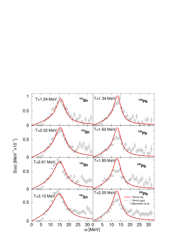
Fig. 2: The IVGDR strength function in ¹²⁰Sn (LHS) and ²⁰⁸Pb (RHS) within the Fermi gas model (dashed lines) and Fermi liquid model (solid lines) at serveral temperatures compared with normalized data from Ref.¹³⁾.

Comparing also the observerd shape evolution of IVGDR strength function with our models underlies the latter fact. In Fig. 2 we have plotted the strength function (22) for ¹²⁰Sn (LHS) and ²⁰⁸Pb (RHS) within the Fermi gas model (11) (dashed lines) and Fermi liquid model (19) (solid lines) with the normalized data from Ref.¹³⁾. The good overall agreement of the shape evolution of both models with the experiment is again accompanied with only minor differences between the Fermi gas and the Fermi liquid model.

References

1) U. Fuhrmann, K. Morawetz and R. Walke: Phys. Rev. C 58, 1472 (1998).

2) S. Ayik and D. Boilley: Phys. Lett. B 276, 263 (1992): ibid. 284, 482(E) (1992).

3) A. A. Abrikosov and I. M. Khalatnikov: Rep. Prog. Phys. 22, 329 (1959).

4) E. M. Lifshitz and L. Pitajevski: Physical Kinetics (Nauka, Moscow, 1978).

5) K. Morawetz and H. S. Köhler: Europhys. J. A (1999), in press.

6) S. Ayik, M. Belkacem, and A. Bonasera: Phys. Rev. C 51, 611 (1995).

7) S. Ayik, O. Yilmaz, A. Gokalp, and P. Schuck: Phys. Rev. C 58, 1594 (1998).

8) V. M. Kolomietz, A. G. Magner, and V. A. Plujko: Z. Phys. A 345, 131 (1993).

9) A. G. Magner, V. M. Kolomietz, H. Hofmann, and S. Shlomo: Phys. Rev. C 51, 2457 (1995).

10) N. D. Mermin: Phys. Rev. B 1, 2362 (1970).

11) E. Ramakrishnan et al.: Phys. Rev. Lett. 76, 2025 (1996).

12) E. Ramakrishnan et al.: Nucl. Phys. A549, 49 (1996).

13) T. Baumann et al.: Nucl. Phys. A635, 428 (1998).