General response function for interacting quantum liquids

Abstract

Linearizing the appropriate kinetic equation we derive general response functions including selfconsistent mean fields or density functionals and collisional dissipative contributions. The latter ones are considered in relaxation time approximation conserving successively different balance equations. The effect of collisions is represented by correlation functions which are possible to calculate with the help of the finite temperature Lindhard RPA expression. The presented results are applicable to finite temperature response of interacting quantum systems if the quasiparticle or mean field energy is parameterized within Skyrme - type of functionals including density, current and energy dependencies which can be considered alternatively as density functionals. By this way we allow to share correlations between density functional and collisional dissipative contributions appropriate for the special treatment. We present results for collective modes like the plasmon in plasma systems and the giant resonance in nuclei. The collisions lead in general to an enhanced damping of collective modes. If the collision frequency is close to the frequency of the collective mode, resonance occurs and the collective mode is enhanced showing a collisional narrowing.

]

I Introduction

The response of matter to an external perturbation is the main source of knowledge about the matter itself. For instance, in plasma physics the polarization function $\Pi(q,\omega)$ is linked via the dielectric function $\epsilon(q,\omega)$ to the electrical conductivity $\sigma(q,\omega)$ by

$$\epsilon(q,\omega)=1-V(q)\Pi(q,\omega)=1+{i\over\omega}\sigma(q,\omega).$$ (1)

In nuclear matter, e.g., the response function $\chi=\Pi/\epsilon$ allows one to study excitations and giant resonances which in turn yields information about the equation of state like the isothermal compressibility which is given by

$$\kappa={1\over n^{2}}\left({\partial n\over\partial\mu}\right)_{T}={1\over n^{2}T}\lim\limits_{q\to 0}\int{d\omega\over\pi}{1\over{\rm e}^{\omega/T}-1}{\rm Im}{\chi(q,\omega)}$$ (2)

(3)

or to calculate fluctuations and diffusion coefficients.

Two lines of theoretical improvements of the response function can be found in print recently. The first one starts from TDHF equations and considers the response of nuclear matter described by a time reversal broken Skyrme interaction [1, 2]. The other line tries to improve the response by the inclusion of collisional correlations [3, 4, 5, 6] and for multicomponent systems [7, 8]. In this paper we want to combine both lines of improvements into one expression and derive therefore the response function from a kinetic equation including mean field (Skyrme) and collisional correlations.

We consider here interacting matter which can be described by an energy functional ( mean field) ${\cal E}$ originally introduced by Skyrme [9, 10] and the residual interaction. The latter one we condense in a collisional integral additional to the TDHF equation. Then the response to an external perturbation will contain the effect of Skyrme mean field and additionally the effect of residual interaction. While this schema and the results are of general interest for any interacting Fermi- or Bose system, we will only mention application examples from nuclear matter and plasma physics. For the latter one we might consider the energy functional as a parameterization of the selfenergy in line with the philosophy of density functional theory. By this way we have the freedom to share the correlations between mean field like density functional parameterizations and explicit collisional or dissipative like correlations which are condensed in a relaxation time. Of course, when deriving this parameterizations microscopically special care is required to avoid double counting of correlations.

Specifically, we want to obtain the density, current and energy response $\chi,\chi_{J},\chi_{E}$ of an interacting quantum system

$$\left(\matrix{\delta n\cr\delta{\bf\nabla J}\cr\delta E}\right)=\left(\matrix{\chi\cr\chi_{J}\cr\chi_{E}}\right)\,\,V^{\rm ext}\equiv{\cal X}\left(\matrix{1\cr 0\cr 0}\right)V^{\rm ext}\equiv{\cal X}\nu^{\rm ext}$$ (4)

(5)

to the external perturbation $V^{\rm ext}$ provided the density, momentum and energy are conserved

$$n({\bf R},t) = \sum\limits_{j}\langle\Phi_{j}^{*}({\bf R})\Phi_{j}({\bf R})\rangle=s\sum\limits_{p}f({\bf p,R},t),$$ (6)

$${\bf J}({\bf R},t) = \sum\limits_{j}\langle{\nabla_{\bf R}-\nabla_{\bf R^{\prime}}\over 2i}\Phi_{j}^{*}({\bf R^{\prime}})\Phi_{j}({\bf R})\rangle_{{\bf R}={\bf R^{\prime}}}$$ (7)

$$= s\sum\limits_{p}{\bf p}f({\bf p,R},t),$$ (8)

$$E({\bf R},t) = \sum\limits_{j}\langle{\cal H}({\bf R},t)\rangle=s\sum\limits_{p}\varepsilon({\bf p,R},t)f({\bf p,R},t).$$ (9)

Here $s$ is the spin-isospin degeneracy and we express the observables in terms of the Wigner function $f({\bf p,R},t)$ which is related to the one-particle density operator $\hat{\rho}$ by

$$f({\bf p,R},t)=\sum\limits_{q}{\rm e}^{i{\bf qR}}\langle p+{q\over 2}|\hat{\rho}|p-{q\over 2}\rangle$$ (10)

and introduce the quasiparticle (Skyrme) energy $\varepsilon$

$$\varepsilon({\bf p,R},t)=\sum\limits_{q}{\rm e}^{i{\bf qR}}\langle p+{q\over 2}|\hat{\cal E}|p-{q\over 2}\rangle$$ (11)

in the spirit of Landau theory $\varepsilon={\delta E\over\delta f}$. We will neglect the contributions of energy gain which arise from noninstantaneous collisions [11]. Here the energy functional or mean field (Skyrme) energy $\varepsilon$ is assumed to be parameterized as [12]

$$\hat{\cal E} = -\nabla({1\over 2m}+\epsilon_{1}n)\nabla+\epsilon_{2}n+\epsilon_{1}[2mE-{1\over i}(\nabla{\bf J}+{\bf J}\nabla)]$$ (13)

$$+\epsilon_{3}\nabla^{2}n+\epsilon_{4}n^{\alpha+1}.$$

Please note that the occurrence of current contributions $\sim{\bf J}$ breaks explicitly the time invariance. These terms appear with the same coefficient $\epsilon_{1}$ as the effective mass and energy contribution in order to ensure Galilean invariance. The density dependence $\alpha\neq 1$ deviating from the one arising by Skyrme three-body contact interaction has been introduced and compared with experiments in [13].

II Derivation of general response function

We start the derivation of the response from the quantum kinetic equation for the density operator in relaxation time approximation

$$\dot{\hat{\rho}}+i[\hat{\cal E}+\hat{V}^{\rm ext},\hat{\rho}]={\hat{\rho}^{\rm l.e.}-\hat{\rho}\over\tau}$$ (15)

where the relaxation is considered with respect to the local density operator $\hat{\rho}^{\rm l.e.}$ or the corresponding local equilibrium distribution function

$$f^{\rm l.e.}({\bf p,R},t)=f_{0}\left({\varepsilon_{0}({\bf p}-{\bf Q}({\bf R},t))-\mu({\bf R},t)\over T({\bf R},t)}\right)$$ (16)

with the (Fermi/Bose) distribution $f_{0}$. This local equilibrium is given by a local chemical potential $\mu$, a local temperature $T$ and a local mass motion momentum $Q$. These local quantities will be specified by the requirement that the expectation values for density, momentum and energy are the same as the expectation values performed with $f$.

A Conservation laws

From (15) we see that the conservation laws for density, momentum and energy are fulfilled if the corresponding expectation value of the collision side vanishes

$$\sum\limits_{p}(f-f^{\rm l.e.}) = 0$$ (17)

$$\sum\limits_{p}{\bf p}(f-f^{\rm l.e.}) = 0$$ (18)

$$\sum\limits_{p}\varepsilon(f-f^{\rm l.e.}) = 0.$$ (19)

Taking this into account we can express the deviation of the observables $\phi=1,{\bf p},\varepsilon$ from equilibrium considering $\delta f=f-f_{0}=f-f^{\rm l.e.}+f^{\rm l.e.}-f_{0}$ as

$$\delta\phi({\bf q},\omega) = \sum\limits_{p}\phi\delta f({\bf p,q},\omega)$$ (20)

$$= \sum\limits_{p}\phi(f^{\rm l.e.}-f_{0})$$ (21)

$$= \sum\limits_{p}\phi{f_{0}({\bf p}+{{\bf q}\over 2})-f_{0}({\bf p}-{{\bf q}\over 2})\over\varepsilon_{0}({\bf p}+{{\bf q}\over 2})-\varepsilon_{0}({\bf p}-{{\bf q}\over 2})}$$ (23)

$$\times\left[-\delta\mu-{\bf q}{\partial\varepsilon_{0}\over\partial{\bf p}}\delta{Q}-{\varepsilon_{0}-\mu\over T}\delta T\right]$$

where we have performed Fourier transform $t\rightarrow-i\omega$ and ${\bf r}\rightarrow i{\bf q}$. In the last line we restrict to linear response of (16). We assume for simplicity a homogeneous equilibrium $f_{0}(\varepsilon_{0}({\bf p}))$ such that only the deviations $\delta\phi({\bf r},t)$ and $\delta f({\bf p,r},t)$ are space dependent. This is no principle restriction but otherwise a lot of later algebraic expressions would take the form of integral equations. Further $\delta{\bf Q}({\bf q},t)={\bf q}\delta Q({\bf q},t)$ is employed. With the abbreviation

$$a_{\phi} = \sum\limits_{p}\phi{f_{0}({\bf p}+{{\bf q}\over 2})-f_{0}({\bf p}-{{\bf q}\over 2})\over\varepsilon_{0}({\bf p}+{{\bf q}\over 2})-\varepsilon_{0}({\bf p}-{{\bf q}\over 2})}$$ (24)

$$= g_{\phi}(0),$$ (25)

$${b}_{\phi} = \sum\limits_{p}\phi{\bf q}{\partial\epsilon\over\partial{\bf p}}{f_{0}({\bf p}+{{\bf q}\over 2})-f_{0}({\bf p}-{{\bf q}\over 2})\over\varepsilon_{0}({\bf p}+{{\bf q}\over 2})-\varepsilon_{0}({\bf p}-{{\bf q}\over 2})}$$ (26)

$$= g_{\phi{\bf q}\partial_{\bf p}\varepsilon_{0}}(0),$$ (27)

$$c_{\phi} = \sum\limits_{p}\phi{\varepsilon_{0}-\mu\over T}{f_{0}({\bf p}+{{\bf q}\over 2})-f_{0}({\bf p}-{{\bf q}\over 2})\over\varepsilon_{0}({\bf p}+{{\bf q}\over 2})-\varepsilon_{0}({\bf p}-{{\bf q}\over 2})}$$ (28)

$$= {1\over T}g_{\phi\varepsilon_{0}}(0)-{\mu\over T}g_{\phi}(0)$$ (29)

and the correlation function

$$g_{\phi}(\omega) = \sum\limits_{p}\phi{f_{0}({\bf p}+{{\bf q}\over 2})-f_{0}({\bf p}-{{\bf q}\over 2})\over\varepsilon_{0}({\bf p}+{{\bf q}\over 2})-\varepsilon_{0}({\bf p}-{{\bf q}\over 2})-\omega-i0}$$ (30)

we can write the deviation of the observables from equilibrium according to (23) explicitly

$$\delta n = -\delta\mu a_{1}-\delta Qb_{1}-\delta Tc_{1},$$ (31)

$$\delta J_{q} = {\bf q}\delta{\bf J}=-\delta\mu a_{\bf qp}-\delta{Q}b_{\bf qp}-\delta Tc_{\bf qp},$$ (32)

$$\delta E = -\delta\mu a_{\epsilon}-\delta Qb_{\epsilon}-\delta Tc_{\epsilon}.$$ (33)

Instead of the vector equation for the current ${\bf J}$ we consider the projection onto the direction of ${\bf q}$. This simplifies matters as long as we have no active media and ${\bf J}||{\bf Q}$.

B Response from kinetic equation

To derive the response function we will obtain a second equation set from linearizing the kinetic equation (15) and the corresponding balance equations. Fourier transform $t\rightarrow-i\omega$ and ${\bf r}\rightarrow i{\bf q}$ the equation (15) can be linearized

$$-i\omega\delta f+i\left[\varepsilon_{0}({\bf p}+{{\bf q}\over 2})-\varepsilon_{0}({\bf p}-{{\bf q}\over 2})\right]\delta f$$ (34)

$$-i\left[f_{0}({\bf p}+{{\bf q}\over 2})-f_{0}({\bf p}-{{\bf q}\over 2})\right]$$ (35)

$$\times\left[V^{\rm ext}+(V_{0}+V_{4}p^{2})\delta n+{\bf pq}V_{1}\delta J_{q}+V_{2}\delta E\right]$$ (36)

$$=-{\delta f\over\tau}$$ (37)

$$+{1\over\tau}{f_{0}({\bf p}+{{\bf q}\over 2})-f_{0}({\bf p}-{{\bf q}\over 2})\over\varepsilon_{0}({\bf p}+{{\bf q}\over 2})-\varepsilon_{0}({\bf p}-{{\bf q}\over 2})}\left[-\delta\mu-{\bf q}{\partial\varepsilon_{0}\over\partial{\bf p}}\delta Q-{\varepsilon_{0}-\mu\over T}\delta T\right].$$ (38)

(39)

In (39) the mean field contributions $V_{i}$ will lead just to selfconsistency. The coefficients $V_{i}$ it-selves are linked to the parameterization (13) as

$$V_{0} = {\delta\varepsilon_{0}\over\delta n}=\epsilon_{2}-\epsilon_{1}{q^{2}\over 2}-\epsilon_{3}q^{2}+(\alpha+1)n_{0}^{\alpha}\epsilon_{4},$$ (40)

$$V_{1} = {\delta\varepsilon_{0}\over\delta{J_{q}}}=-{2\epsilon_{1}\over q^{2}},$$ (41)

$$V_{2} = {\delta\varepsilon_{0}\over\delta E}=2m\epsilon_{1},$$ (42)

$$V_{4} = \epsilon_{1}.$$ (43)

We can solve (39) for $\delta f$ and perform momentum integrations to obtain the observables $\delta n$, $\delta J_{q}$, $\delta E$. This leads to the following closed equation system

$${\cal I}\left(\matrix{\delta n\cr\delta J_{q}\cr\delta E}\right)={\cal B}\left(\matrix{\delta\mu\cr\delta Q\cr\delta T}\right)+{\cal V}\left(\matrix{\delta n\cr\delta J_{q}\cr\delta E}\right)+\left(\matrix{g_{1}\cr g_{\bf pq}\cr g_{\epsilon}}\right)V^{\rm ext}$$ (44)

together with the set (33)

$$\left(\matrix{\delta n\cr\delta J_{q}\cr\delta E}\right)={\cal A}\left(\matrix{\delta\mu\cr\delta Q\cr\delta T}\right).$$ (45)

The matrices are

$${\cal V} = \left(\matrix{g_{1}V_{0}+g_{p^{2}}V_{4}&g_{\bf pq}V_{1}&g_{1}V_{2}\cr g_{\bf pq}V_{0}+g_{p^{2}{\bf pq}}V_{4}&g_{({\bf pq})^{2}}V_{1}&g_{\bf pq}V_{2}\cr g_{\epsilon}V_{0}++g_{p^{2}\epsilon}V_{4}&g_{\epsilon{\bf pq}}V_{1}&g_{\epsilon}V_{2}}\right)_{\omega+{i\over\tau}}$$ (46)

$${\cal B} = -\left(\matrix{d_{1}&e_{1}&f_{1}\cr d_{\bf pq}&e_{\bf pq}&f_{\bf pq}\cr d_{\epsilon}&e_{\epsilon}&f_{\epsilon}}\right)$$ (47)

$${\cal A} = -\left(\matrix{a_{1}&b_{1}&c_{1}\cr a_{\bf pq}&b_{\bf pq}&c_{\bf pq}\cr a_{\epsilon}&b_{\epsilon}&c_{\epsilon}}\right)$$ (48)

and the abbreviations are introduced

$$d_{\phi} = {-i\over\omega\tau+i}\left[g_{\phi}(\omega+{i\over\tau})-g_{\phi}(0)\right],$$ (49)

$$e_{\phi} = {-i\over\omega\tau+i}\left[g_{\phi{\bf q}\partial_{\bf p}\epsilon}(\omega+{i\over\tau})-g_{\phi{\bf q}\partial_{\bf p}\epsilon}(0)\right],$$ (50)

$$f_{\phi} = {-i\over\omega\tau+i}{1\over T}\left(g_{\phi\epsilon}(\omega+{i\over\tau})-g_{\phi\epsilon}(0)\right.$$ (52)

$$\left.-\mu\left[g_{\phi}(\omega+{i\over\tau})-g_{\phi}(0)\right]\right)$$

in terms of the correlation function (30). The required solution is obtained from (44) and (45) as

$$\left(\matrix{\delta n\cr\delta J_{q}\cr\delta E}\right)=({\cal I}-{\cal V}-{\cal B}{\cal A}^{-1})^{-1}\left(\matrix{g_{1}\cr g_{\bf pq}\cr g_{\epsilon}}\right)V^{\rm ext}$$ (54)

from which one can read off the response functions (5). This is the main result of the paper which represents the density, momentum and energy response including nonlinear mean fields and collisions with the fulfillment of density -, momentum -, and energy - conservation.

C Alternative expressions

Before we continue to consider special cases we like to express the solution (54) in a slightly more familiar form.

1 Response in terms of mean-field response

First we assume that we have solved the response without collisions ${\cal B}=0$ which would obey the equation

$$({\cal I}-{\cal V})\xi_{0}={\cal G}\nu^{ext}$$ (55)

where $\xi={\{}\delta n,\delta J_{q},\delta E{\}}$, $\nu^{ext}={\{}V^{\rm ext},0,0{\}}$ and

$${\cal G}(\omega)=\left(\matrix{g_{1}&g_{\bf pq}&g_{\epsilon}\cr g_{\bf pq}&g_{({\bf pq})^{2}}&g_{{\bf pq}\epsilon}\cr g_{\epsilon}&g_{\epsilon{\bf pq}}&g_{\epsilon\epsilon}}\right).$$ (56)

Than the response matrix (5) without collisions but selfconsistent mean field reads

$${\cal X}_{\rm MF}(\omega)=(1-{\cal V})^{-1}{\cal G}(\omega).$$ (57)

The missing part of the full solution of (44,45) including the collisions are given by $\xi=\xi_{0}+\zeta$ where we have for $\zeta$

$$(1-{\cal V}-{\cal BA}^{-1})\zeta={\cal BA}^{-1}\xi_{0}.$$ (58)

Some algebra leads to the final response

$${\cal X}(\omega)=$$ (59)

$${\cal X}_{\rm MF}(\omega+{i\over\tau})\left(1-{\cal G}^{-1}(\omega+{i\over\tau}){\cal BA}^{-1}{\cal X}_{\rm MF}(\omega+{i\over\tau})\right)^{-1}.$$ (60)

(61)

2 Response in terms of polarization function

The opposite case is the usual way where we first solve the equation without selfconsistency by the mean field. This leads to the polarization function ${\cal P}=\{\Pi,\Pi_{J},\Pi_{E}\}$ which we use to represent the response function which includes selfconsistency. Without mean field we have from (54)

$$({\cal I}-{\cal BA}^{-1})\xi_{0}={\cal G}\nu^{ext}$$ (62)

leading to the polarization function

$${\cal P}(\omega)=(1-{\cal BA}^{-1})^{-1}{\cal G}(\omega+{i\over\tau}).$$ (63)

The response function can be represented analogously to (61)

$${\cal X}(\omega)={\cal P}(\omega)\left\{{\cal I}-{\cal G}^{-1}(\omega+{i\over\tau})\,{\cal V}\,{\cal P}(\omega)\right\}^{-1}.$$ (64)

(65)

The generalization of the usual form $\chi=\Pi/(1-V\Pi)$ for simple mean fields can be recognized.

III Calculation of response functions

In the following we consider some frequently occurring situations. Therefore we assume only quadratic dispersions $\varepsilon=p^{2}/2m$ in the correlation function. To consider the full quasiparticle (Skyrme) energy would correspond to the selfconsistent quasiparticle RPA which we do not want to consider here. The schema how to include this is clear after the following considerations. We understand in the following the mass as effective mass given by $\epsilon_{1}$ in (13).

The different occurring correlation functions (30) can be written in terms of moments of the usual Lindhard polarization function $\Pi_{0}$

$$\Pi_{n}=\int{d{\bf p}\over(2\pi)^{3}}p^{n}{f_{0}({\bf p}+{{\bf q}\over 2})-f_{0}({\bf p}-{{\bf q}\over 2})\over{{\bf pq}\over m}-\omega-i0}$$ (66)

as following:

$$g_{1} = \Pi_{0}$$ (67)

$$g_{\bf pq} = m\omega\Pi_{0}$$ (68)

$$g_{\epsilon} = {\Pi_{2}\over 2m}$$ (69)

$$g_{\epsilon p^{2}} = {\Pi_{4}\over 2m}$$ (70)

$$g_{p^{2}{\bf pq}} = m\omega\Pi_{2}$$ (71)

$$g_{({\bf pq})^{2}} = -2mq^{2}{n\over s}+m^{2}\omega^{2}\Pi_{0}.$$ (72)

For practical and numerical calculations we can rewrite the $\Pi_{n}$ by polynomial division into

$$\Pi_{2} = -m{n\over s}+{m^{2}\omega^{2}\over q^{2}}\Pi_{0}+\tilde{\Pi}_{2}$$ (73)

$$\Pi_{4} = -{14\over 3}m^{2}{E_{0}\over s}-{nmq^{2}\over 4s}(1+{4m^{2}\omega^{2}\over q^{4}})-{m^{4}\omega^{4}\over q^{4}}\tilde{\Pi}_{0}$$ (75)

$$-{2m^{2}\omega^{2}\over q^{2}}\tilde{\Pi}_{2}-\tilde{\Pi}_{4}$$

where the $\tilde{\Pi}_{i}$ are the projected moments perpendicular to ${\bf q}$ and read

$$\tilde{\Pi}_{2} = \int{d{\bf p}\over(2\pi)^{3}}({\bf p}-{{\bf pq}\over q^{2}}{\bf q})^{2}{f_{0}({\bf p}+{{\bf q}\over 2})-f_{0}({\bf p}-{{\bf q}\over 2})\over{{\bf pq}\over m}-\omega-i0}$$ (76)

$$= 2m\int\limits_{-\infty}^{\mu}d\mu^{\prime}\Pi_{0}$$ (77)

$$\approx 2mT\Pi_{0}$$ (78)

$$\tilde{\Pi}_{4} = \int{d{\bf p}\over(2\pi)^{3}}({\bf p}-{{\bf pq}\over q^{2}}{\bf q})^{4}{f_{0}({\bf p}+{{\bf q}\over 2})-f_{0}({\bf p}-{{\bf q}\over 2})\over{{\bf pq}\over m}-\omega-i0}$$ (79)

$$= 2(2m)^{2}\int\limits_{-\infty}^{\mu}d\mu^{\prime}\int\limits_{-\infty}^{\mu^{\prime}}d\mu^{\prime\prime}\Pi_{0}$$ (80)

$$\approx 8m^{2}T^{2}\Pi_{0}.$$ (81)

The corresponding last identities are valid only for nondegenerate, Maxwellian, distributions with temperature $T$. The general form of polarization functions is presented as an integral over the chemical potential $\mu$ of the Lindhard polarization $\Pi_{0}$. This is applicable also to the degenerate case. In the following we will discuss successively further involved results; first for nondegenerate plasmas and then for degenerate nuclear matter.

A Polarization with collisions: inclusion of density and energy conservation

Now we concentrate on the response function without mean field and consider only the collisions within density and energy conservation. Then the matrices ${\cal A}$ and ${\cal B}$ reduces to 2x2 matrices. The calculation of (62) leads to

$$\Pi^{\rm n,E}(\omega) = (1-i\omega\tau)\left({g_{1}(\omega+{i\over\tau})g_{1}(0)\over h_{1}}\right.$$ (83)

$$\left.-\omega\tau i{(h_{\epsilon}g_{1}(0)-h_{1}g_{\epsilon}(0))^{2}\over h_{1}(h_{\epsilon}^{2}-h_{\epsilon\epsilon}h_{1})}\right)$$

where we use the abbreviation

$$h_{\phi}=g_{\phi}(\omega+{i\over\tau})-\omega\,\tau\,i\,g_{\phi}(0).$$ (84)

With the help of (72-81) this can be further worked out in terms of $\Pi_{n}$ but leads not to a more transparent form. Let us note that the first term in (83) represents just the result if we would have considered only density conservation known as the Mermin polarization function [3]

$$\Pi^{\rm n}(\omega) = (1-i\omega\tau){g_{1}(\omega+{i\over\tau})g_{1}(0)\over h_{1}}.$$ (85)

Of course the limit of vanishing collisions $\tau\rightarrow\infty$ ensures that the Lindhard result $\Pi_{0}(\omega)$ appears since

$$\lim\limits_{\tau\to\infty}{h_{\phi}\over 1-i\omega\tau}=g_{\phi}(0).$$ (86)

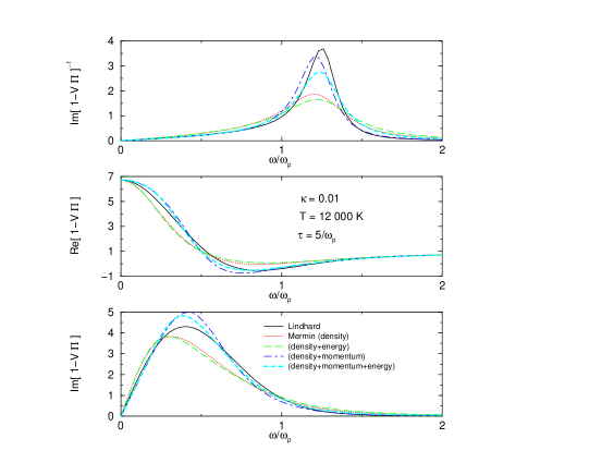
FIG. 1.: The dielectric function $\varepsilon=1-V\Pi$ for a one component plasma system in different approximations. The inverse Debye length is $\kappa^{2}={4\pi ne^{2}\over T}$ and the energy $\omega$ is scaled in plasma frequencies $\omega_{p}^{2}=\kappa^{2}T/m$. The relaxation time is chosen arbitrarily as $\tau=5/\omega_{p}$ and the wave vector $q=0.384\kappa$. The upper most panel shows the excitation function.

B Polarization with collisions: inclusion of density and momentum conservation

Next we consider the special case that the density and momentum are conserved. Then the matrices ${\cal A}$ and ${\cal B}$ reduces again to 2x2 matrices and the calculation of (62) leads to

$$\Pi^{\rm n,J}(\omega) = (1-i\omega\tau){g_{1}(\omega+{i\over\tau})-{\left(g_{\bf pq}(\omega+{i\over\tau})\right)^{2}\over h_{({\bf pq})^{2}}}\over h_{1}-{\left(g_{\bf pq}(\omega+{i\over\tau})\right)^{2}\over h_{({\bf pq})^{2}}}}g_{1}(0).$$ (87)

We have used the fact that according to (72) $g_{\bf pq}(0)=g_{\epsilon{\bf pq}}(0)=0$ and $h_{\phi}$ is defined as in (84). With the help of (1) we obtain by this way a slightly modified Mermin dielectric function (85).

C Polarization with collisions: inclusion of density, momentum and energy conservation

Considering all three conservation laws the result from (65) is

$$\Pi^{\rm n,J,E}(\omega)=(i\omega\tau-1)\left(i\omega\tau{N\over D}-g_{1}[0]\right),$$ (88)

with

$$N= -\left\{g_{\epsilon{\bf pq}}[\omega+{i\over\tau}]g_{1}[0]-g_{\epsilon}[0]g_{\bf pq}[\omega+{i\over\tau}]\right\}^{2}$$ (91)

$$+h_{({\bf pq})^{2}}\left\{g_{1}[0]\left(h_{\epsilon^{2}}g_{1}[0]-h_{\epsilon}g_{\epsilon}[0]\right)\right.$$

$$\left.\quad\qquad+g_{\epsilon}[0]\left(h_{1}g_{\epsilon}[0]-h_{\epsilon}g_{1}[0]\right)\right\}$$

$$D = g_{\epsilon{\bf pq}}[\omega+{i\over\tau}]\left\{h_{1}g_{\epsilon{\bf pq}}[\omega+{i\over\tau}]-h_{\epsilon}g_{\bf pq}[\omega+{i\over\tau}]\right\}$$ (92)

$$+ g_{\bf pq}[\omega+{i\over\tau}]\left\{h_{\epsilon\epsilon}g_{\bf pq}[\omega+{i\over\tau}]-h_{\epsilon}g_{\epsilon{\bf pq}}[\omega+{i\over\tau}]\right\}$$ (93)

$$+ h_{({\bf pq})^{2}}\left\{h_{\epsilon}^{2}-h_{\epsilon\epsilon}h_{1}\right\}.$$ (94)

This result together with the former special cases (85,83,87) are compared in figure 1. One sees that the first approximation of Mermin (85) is almost identical with the result (83) where density and energy is conserved. The inclusion of density and momentum conservation (87) brings the curves towards the Lindhard result without collisions compared with the inclusion of density conservation only. Finally, the complete result with the inclusion of density, momentum and energy conservation (88) changes the results again in the direction of the result for density and energy conservation but less pronounced. This qualitative behavior of the different approximations are observed for other relaxation times too.

The effect of relaxation times within the complete result (88) is seen in figure 2. One recognizes that with decreasing relaxation time or increasing collision frequency the plasmon peak is shifted towards smaller energies. For collision frequencies around the inverse plasma frequency there occurs a resonance seen in the real part of the dielectric function (middle part of 2). This translates into an enhanced single particle damping (lower panel) and the system becomes optical thick. At the same time the collective mode, the plasma frequency, becomes enhanced. One can consider this as an effect of transferring collisional energy into collective motion. We have here a coherent superposition between collision frequency and collective frequency resulting into an enhancement of collective motion. Compared with the general effect of collisions to increase the damping of collective motion, see figure 1, this is the inverse effect which narrows the collective peak again.

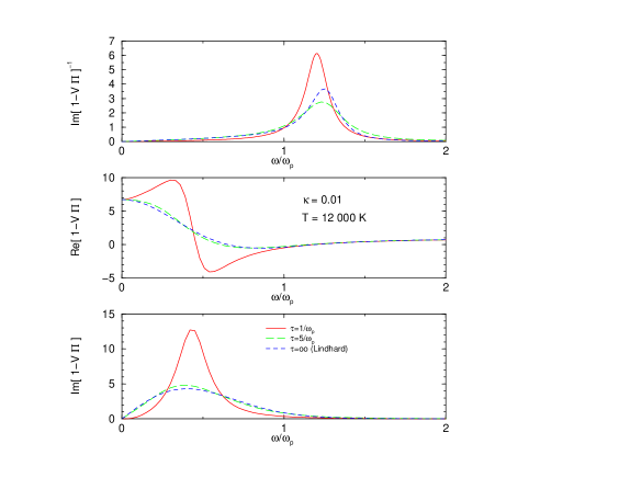
FIG. 2.: The dielectric function $\varepsilon=1-V\Pi$ for a one component plasma system with the inclusion of density, momentum and energy conservation (88) for different relaxation times. The parameter are the same as in figure 1.

D Response with collisions: simple mean field

For the case of simple but density - dependent mean fields $V_{0}\neq 0$ and $V_{1}=V_{2}=V_{4}=0$ we obtain for the density response from (65)

$$\chi={\Pi\over 1-V_{0}\Pi}.$$ (95)

Here $\Pi$ is the polarization function without mean field but with collisions. Dependent on the choice one may use (83), (87) or (88) for the latter one.

Since the imaginary part of the response function (95) is related to the photoabsorbtion yield on nuclei we like to apply the different approximations (83), (87) or (88) for nuclear isovector oscillations. We use first a simplified Skyrme parameterization [14] for $V_{0}$ according to (107) and a relaxation time $\tau$ within a Fermi liquid model [15, 16]. From Fig. 3 we see the same qualitative behavior of the different approximations as found in Fig. 1. The difference between the density (density-momentum) and density-energy (density-energy- momentum) result is very small (inlays of Fig. 3). An increase of temperature leads to larger damping of all approximations (bottom of Fig. 3). While the density or density-energy result leads to a pronounced damping of the giant resonance the inclusion of momentum conservation diminishes this effect again towards the free result.

Let us note that the energy-weighted sum rule (EWSR)

$$-\frac{1}{\pi}\int_{0}^{\infty}d\omega\,\omega\,{\rm Im}\chi=\frac{q^{2}}{2m}n_{0}$$ (96)

is fulfilled numerically for all approximations, however, the convergence is very bad for response including density or density and energy conservation. The inclusion of momentum conservation in turn improves the convergence of the sum rule appreciable.

FIG. 3.: The imaginary part of the response function ${\rm Im}\chi$ for nuclear giant dipole resonances in different approximations (comp. Fig. 1). The wave vector $q=0.23\,{\rm fm}^{-1}$ ($\approx 0.17\,{\rm k}_{F}$) corresponds to the inverse diameter of the nucleus ²⁰⁸Pb according to [17]. The inlays show an enlarged view of the difference between the density (n),density- energy (n-E) and density-momentum (n-p), density-momentum-energy (n-p-E) approximation, respectively.

E Response without collisions: Skyrme mean field

First we consider the case that we have only Skyrme - mean fields. Then the matrix equation (55) is solved with the result for the density response function

$$\chi_{\rm MF}(\omega,V_{i})=$$ (97)

$${\Pi_{0}\over 1-\Pi_{0}{\bar{V}_{0}}+{V_{2}V_{4}\over 2m}\left[\Pi_{2}^{2}-\Pi_{0}\Pi_{4}\right]-\Pi_{2}\left[{V_{2}\over 2m}+V_{4}\right]}$$ (98)

(99)

with

$${\bar{V}_{0}}=V_{0}+{m\omega(m\omega V_{1}+V_{3})\over 2{n\over s}mq^{2}V_{1}+1}.$$ (100)

For isovectorial oscillations one has

$$V_{0} = {\delta\varepsilon_{0}\over\delta n}=V_{0}^{s}-V_{1}^{s}{q^{2}\over 2}$$ (101)

$$V_{1} = {\delta\varepsilon_{0}\over\delta{J_{q}}}=-{2\over q^{2}}V_{1}^{s}$$ (102)

$$V_{2} = {\delta\varepsilon_{0}\over\delta E}=2mV_{1}^{s}$$ (103)

$$V_{4} = V_{1}^{s}$$ (104)

where the $V_{i}^{s}$ are representing the Skyrme parameterization in nuclear matter [1]

$$V_{0}^{s} = -t_{0}(x_{0}+\frac{1}{2})-{t_{3}\over 6}(x_{3}+\frac{1}{2})n^{\alpha}_{0}$$ (106)

$$-{q^{2}\over 16}[3t_{1}(1+2x_{1})+t_{2}(1+2x_{2})]$$

$$V_{1}^{s} = {1\over 8}[t_{2}(1+2x_{2})-t_{1}(1+2x_{1})].$$ (107)

If we use the definitions of [1] which are related to ours as

$$\tilde{\Pi}_{0} = \Pi_{0}$$ (108)

$$\tilde{\Pi}_{2} = \Pi_{2}-{q^{2}\over 4}\Pi_{0}$$ (109)

$$\tilde{\Pi}_{4} = \Pi_{4}-{q^{2}\over 2}\Pi_{2}+{q^{4}\over 16}\Pi_{0}$$ (110)

we obtain the result of [1] which was slightly misprinted

$$\chi_{\rm MF}={\Pi_{0}\over 1-\tilde{\Pi}_{0}\tilde{V}_{0}^{s}-2V_{1}^{s}\tilde{\Pi}_{2}+{(V_{1}^{s})^{2}}\left[\tilde{\Pi}_{2}^{2}-\tilde{\Pi}_{0}\tilde{\Pi}_{4}\right]}$$ (111)

with

$$\tilde{V}_{0}^{s}=V_{0}^{s}-{m^{2}\omega^{2}\over q^{2}}{2V_{1}^{s}\over 1-n_{0}mV_{1}^{s}}$$ (112)

for nuclear matter density $n_{0}$ and $s=4$.

F Response with collisions: inclusion of density conservation and Skyrme mean field

Now we derive the combined result from the mean field response (99) and collisions. We restrict first only on density balance conservation [first term of (83)] to get from (23)

$$\delta\mu=-{\delta n\over a_{1}}=-{\delta J_{q}\over a_{\bf pq}}=-{\delta E\over a_{\epsilon}}$$ (113)

and in (54)

$${\cal BA}^{-1}=\left(\matrix{{d_{1}\over a_{1}}&0&0\cr 0&{d_{\bf pq}\over a_{\bf pq}}&0\cr 0&0&{d_{\epsilon}\over a_{\epsilon}}}\right).$$ (114)

Therefore we can solve (65) and obtain similar to (99)

$$\chi^{\rm n}(\omega)=$$ (115)

$$(1-i\omega\tau){g_{1}(0)\over h_{1}}\chi_{\rm MF}(\omega+{i\over\tau},\tilde{V}_{i})$$ (116)

with

$$\tilde{V}_{0} = (1-i\omega\tau){g_{1}(0)\over h_{1}}V_{0}$$ (117)

$$\tilde{V}_{1} = (1-i\omega\tau){g_{\bf pq}(0)\over h_{\bf pq}}V_{1}=\left\{\matrix{V_{1}+o(\omega\tau)^{-1}\cr 0+o(\omega\tau)}\right.$$ (118)

$$\tilde{V}_{2} = (1-i\omega\tau){g_{\epsilon}(0)\over h_{\epsilon}}V_{2}$$ (119)

$$\tilde{V}_{4} = (1-i\omega\tau){g_{1}(0)\over h_{1}}V_{4}.$$ (120)

We should note that the mean field potential $V_{1}$ arising from current and effective mass is of a different level of approximation than the collisional contribution which we restricted in (114) to the density conservation. This inconsistency is visible in the final result for $\tilde{V}_{1}$ in (120) where the limit of vanishing collisions $\tau\to\infty$ does not agree with the limit of finite collisions since $g_{\bf pq}(0)\equiv 0$, see (72). Therefore $\tilde{V}_{1}=V$ is proposed to ensure the limit of vanishing collisions.

FIG. 4.: The imaginary part of the response function ${\rm Im}\chi$ for nuclear giant dipole resonances (see Fig. 4) in different approximations. Considering the Skyrme interactions SGII [1, 18] we compare the full mean field response with collisional correlations in density (dotted line) and density, momentum and energy approximation (dashed line), respectively, with the collision-free mean field response (solid line) for two different temperatures.

G Response with collisions: inclusion of density, momentum and energy conservation and Skyrme mean field

The Skyrme response can be given also for the other cases including energy and momentum conservation. However this leads not to a more transparent form than the general matrix structure (65). Considering the standard effective Skyrme interaction SGII [18] in figure 4 we compare the complete result (54) including energy, momentum and density conservation (dashed line) with the result including only density conservation (116) (dotted line). In the latter one we have proposed for $\tilde{V}_{1}$ the collision-free value $V_{1}$ in order to ensure the correct limiting case.

We find again the same behavior for the different approximations as in the case of the simplified mean field (Fig. 3). The inclusion of collisions leads to an enhanced damping and a shift of the collective peak towards smaller energies. This effect of collisions is less pronounced by the full mean field result including density, momentum and energy conservation (solid line). The increase of temperature leads to a broadening of the resonance structure (lower part of Fig. 3) in any case.

Again we have checked our results to satisfy the EWSR

$$-\frac{1}{\pi}\int_{0}^{\infty}d\omega\,\omega\,{\rm Im}\chi=\frac{q^{2}}{2m}n_{0}(1+\kappa),$$ (121)

with the enhancement factor $\kappa$

$$\kappa=\frac{m}{4}\left[t_{1}(2+x_{1})+t_{2}(2+x_{2})\right]n_{0}.$$ (122)

Here $\kappa$ occurs as a consequence of the momentum-dependent terms in the Skyrme interaction and is defined as the deviation from the Thomas-Reiche-Kuhn sum rule in the case of isovector giant dipole resonance [19, 20].

The result (99) which contains the full Skyrme mean field but no collisions is in excellent agreement with (121). The approximation (116) including collisions but only density conservation conserves the sum rule only $\approx 75\%$ which is a consequence of the inconsistency of (120). The inclusion of density, momentum and energy conservation (54) conserves the sum rule (121) again completely.

IV Summary

In this paper we have derived the unifying response function including nonlinear mean fields (Skyrme) and collisional correlations. Within this approach one can share correlations between an energy functional of mean field (Skyrme) parameterization and explicit dissipative correlations condensed in the relaxation time. This allows to treat also dissipative effects in density functional approaches. We see that the known limiting cases are reproduced neglecting either collisions or mean fields. Special transparent cases of the unifying response are discussed.

For a nondegenerate plasma numerical results are presented. The first order correction given by the Mermin response, incorporating only the density balance, is similar to the approximation where density and energy are conserved. The plasmon peak is shifted towards smaller frequencies. This is accompanied by an enhanced damping. The incorporation of momentum balance diminishes this effect of collisions.

We observe that an enhancement of the collective mode occurs for collision frequencies near the collective (plasma) frequency. This is the inverse effect of damping due to collisions in that the collisions become resonant and the collective mode is enhanced. We consider this as collisional narrowing. Since the momentum conservation is responsible for that effect we suggest that the physical origin is the same as sometimes discussed with motional narrowing. We like to stress that this narrowing is observed relative to the broadened mode due to collisions and did not reach the collision - free value. Consequently we have collisional damping every time but near the resonant situation this collisional damping is diminished.

Similar behavior is found for the case of nuclear matter, where the collective mode is the giant resonance. For isovectorial giant resonances we checked the extended energy weighted sum rules and find excellent completion. The response due to nonlocal mean fields is derived including the effect of collisional correlations.

REFERENCES

• [1] F. Braghin, D. Vautherin, and A. Abada, Phys. Rev. C 52, 2504 (1995).
• [2] E. Hernández, J. Navarro, A.Polls, and J. Ventura, Nucl. Phys. A597, 1 (1996).
• [3] N. Mermin, Phys. Rev. B 1, 2362 (1970).
• [4] H. Heiselberg, C. J. Pethick, and D. G. Ravenhall, Ann. Phys. 223, 37 (1993).
• [5] D. Kiderlen and H. Hofmann, Phys. Lett. B 332, 8 (1994).
• [6] G. Röpke and A. Wierling, Phys. Rev. E 57, 7075 (1998).
• [7] K. Morawetz, R. Walke, and U. Fuhrmann, Phys. Rev. C 57, R 2813 (1998).
• [8] F. Braghin, Phys. Lett. B 446, 1 (1999).
• [9] T. H. R. Skyrme, Phil. Mag. 1, 1043 (1956).
• [10] T. H. R. Skyrme, Nucl. Phys. 9, 615 (1959).
• [11] P. Lipavský, V. Špička, and K. Morawetz, Phys. Rev. E 52, R1291 (1999).
• [12] Y. Engel et al., Nucl. Phys. A 249, 215 (1975).
• [13] H. S. Köhler, Nucl. Phys. A 258, 301 (1976).
• [14] F. Braghin and D. Vautherin, Phys. Lett. B 333, 289 (1994).
• [15] U. Fuhrmann, K. Morawetz, and R. Walke, Phys. Rev. C. 58, 1473 (1998).
• [16] K. Morawetz and U. Fuhrmann, in Proceedings of the Riken Symposium on Nuclear Collective Excitations,Saitama, March 1999.
• [17] H. Steinwedel and J. Jensen, Z. Naturforsch. 5, 413 (1950).
• [18] N. V. Giai and N. Sagawa, Nucl. Phys. A 371, 1 (1981).
• [19] P. Q. J. Meyer and B. K. Jennings, Nucl. Phys. A 385, 103 (1982).
• [20] J. M. P. Gleissl, M. Brack and P. Quentin, Ann. Phys. (NY) 197, 205 (1990).