ISGDR- bulk or surface mode ?

The existence of isoscalar giant dipole resonance (ISGDR) in nuclear matter is considered as a spurious mode in most text books since one associates with it a center of mass motion. The more surprising was the experimental justification of a giant resonance carrying the quantum numbers of a isoscalar and dipole mode¹⁾²⁾. Consequently one has to consider higher harmonics as explanation of such a mode¹⁾³⁾⁴⁾. Usually this mode is associated with a squeezing mode analogous to a sound wave¹⁾²⁾⁵⁾.

In this letter we want to discuss the influence of surface effects on the ISGDR compression mode. We will show that even in the frame of the Fermi liquid model such mode can be understood. Moreover we claim that the surface effects are not negligible for reproducing the strength function. Consequently we give first a short derivation of response function including surface effects. This will result into a new formula on the level of temperature dependent extended Thomas Fermi approximation⁶⁾.

The starting point is the semiclasssical Vlasov equation

$$\partial_{t}f+{{\bf p}\over m}{\bf\nabla}_{R}{\bf\nabla}_{p}f-{\bf\nabla}_{R}(U^{\rm ext}+U^{\rm ind}){\bf\nabla}_{p}f=0$$ (1)

where $U^{\rm ext}$ is the external perturbation and $U^{\rm ind}$ the selfconsistent meanfield. Provided we know the response to the external potential without selfconsistent meanfield, which is described by the polarization function $\Pi$

$$\delta n({\bf x},t)=\int d{\bf x}^{\prime}\Pi({\bf x,x^{\prime}},t)U^{\rm ext}({\bf x^{\prime}},t).$$ (2)

The response including meanfield $\chi$, is given by

$$\chi({\bf x,x^{\prime}},t)=\Pi({\bf x,x^{\prime}},t)$$

$$+\int d{\bf x}_{1}d{\bf x}_{2}\Pi({\bf x},{\bf x}_{1},t){\delta U^{\rm ind}({\bf x}_{1},t)\over\delta n({\bf x}_{2},t)}\chi({\bf x}_{2},{\bf x^{\prime}},t).$$ (3)

Therefore we concentrate first on the calculation of the polarization function $\Pi$ and linearize the Vlasov equation (1) according to

$$f({\bf p,R},t)=f_{0}({\bf p,R})+\delta f({\bf p,R},t)$$ (4)

such that the induced density variation $\delta n({\bf R},t)=$
$\int\frac{d{\bf p}}{(2\pi\hbar)^{3}}\delta f$ reads

$$\delta n({\bf x},\omega)=\int{d{\bf q}\over(2\pi\hbar)^{3}}{\rm e}^{i{\bf qx}}$$

$$\times\int{d{\bf p}d{\bf x^{\prime}}\over(2\pi\hbar)^{6}}{\rm e}^{-i{\bf qx^{\prime}}}{{\bf\nabla}_{p}f_{0}({\bf p,x^{\prime}}){\bf\nabla}_{x^{\prime}}U^{\rm ext}({\bf x^{\prime}},t)\over i(\omega-{{\bf pq}\over m})}.$$

(5)

Here we have employed the Fouriertransform of space and time coordinates of (1) to solve for $\delta f$ and inverse transform the momentum into the form (5). Comparing (5) with the definition of the polarization function (2) we extract with one partial integration

$$\Pi({\bf x,x^{\prime}},\omega)=-{\bf\nabla}_{x^{\prime}}\int{d{\bf p}d{\bf q}\over(2\pi\hbar)^{6}}{\rm e}^{i{\bf q}({\bf x-x^{\prime}})}{{\bf\nabla}_{p}f_{0}({\bf p,x^{\prime}})\over i(\omega-{{\bf pq}\over m})}.$$ (6)

With (6) and (3) we have given the polarization and response functions for a finite system.

In the following we are interested in the gradient expansion since we believe that the first order gradient terms will bear the information about surface effects. Therefore we change to center of mass and difference coordinates ${\bf R}=({\bf x}_{1}+{\bf x}_{2})/2$, ${\bf r}={\bf x}_{1}-{\bf x}_{2}$ and retaining only first order gradients we get from (6) after Fourier transform of ${\bf r}$ into ${\bf q}$

$$\Pi({\bf R,q})=-\int{d{\bf p}\over(2\pi\hbar)^{3}}{{\bf q\nabla}_{p}f_{0}({\bf p,R})\over\omega-{{\bf pq}\over m}}$$

$$+{i\over 2}{\bf\nabla}_{R}\int{d{\bf p}\over(2\pi\hbar)^{3}}\biggl{(}{{\bf\nabla}_{p}f_{0}({\bf p,R})\over\omega-{{\bf pq}\over m}}-{{\bf p}\over m}{{\bf q.\nabla}_{p}f_{0}({\bf p,R})\over(\omega-{{\bf pq}\over m})^{2}}\biggr{)}$$

$$=-\int{d{\bf p}\over(2\pi\hbar)^{3}}[{\bf q}-i{\bf\nabla}_{R}(1+{\omega\over 2}\partial_{\omega})]{{\bf\nabla}_{p}f_{0}({p^{2}\over 2m},{\bf R})\over\omega-{{\bf pq}\over m}}$$ (7)

where in the last equality we have assumed radial momentum dependence of the distribution function $f_{0}$. We recognize that besides the usual Lindhard polarization function as the first part of (7) we obtain a second part which is expressed by a gradient in space. The first part corresponds to the Thomas Fermi result where we have to use the spatial dependence in the distribution functions and the second part represents the extended Thomas Fermi approximation. So far we did not assume any special form of the distribution function. Therefore the expression (7) is as well valid for any high temperature polarization of finite systems.

What remains is to show that the response function (3) does not contain additional gradients. This is easily confirmed by two equivalent formulations of (3), $\Pi^{-1}\chi=1+V\chi$ and $\chi\Pi^{-1}=1+\chi V$, which by adding yield the anticommutator

$$[\Pi^{-1},\chi]_{+}=2+[V,\chi]_{+}.$$ (8)

This anticommutator does not contain any gradients up to second order. Therefore we have [$V={\delta U^{\rm ind}/\delta n}$]

$$\chi({\bf R,q},\omega)={\Pi({\bf R,q},\omega)\over 1-V({\bf R,q},\omega)\Pi({\bf R,q},\omega)}+{\cal O}(\partial_{R}^{2}).$$ (9)

Equation (9) and (7) give the response and polarization functions of finite systems in first order gradient approximation.

Now we are ready to derive approximate formulae for spherical nuclei. In this case we can assume ${\bf q}||{\bf R}$ and we have

$$\Pi(R,{\bf q},\omega)=\Pi^{0}(R,{\bf q},\omega)-{i\over q}\partial_{R}\left[1+{\omega\over 2}\partial_{\omega}\right]\Pi^{0}(R,{\bf q},\omega)$$

(10)

where $\Pi_{0}$ is the usual Lindhard polarization with spatial dependent distributions (chemical potentials, density). We use now further approximations. In the case of giant resonances we are in the regime where ${\rm Im}\Pi^{0}\sim\omega$ such that

$$\left[1+{\omega\over 2}\partial_{\omega}\right]\Pi^{0}=i\frac{3}{2}{\rm Im}\Pi^{0}$$ (11)

and for small $q$ the real part vanishes for ${\rm Re}\Pi^{0}\sim 1-c^{2}q^{2}/\omega^{2}$. Within the local density approximation we know that the spatial dependence is due to the density $n(R)=n_{0}\Theta(R_{0}-R)$. Since we have for zero temperature ${\rm Im}\Pi^{0}\propto p_{f}(n)$ we evaluate

$$\partial_{R}{\rm Im}\Pi^{0} = -n_{0}\delta(R_{0}-R)\partial_{n}{\rm Im}\Pi^{0}$$ (12)

$$= -\frac{1}{3}\delta(R_{0}-R){\rm Im}\Pi^{0}$$

where we assumed the density dependence carried only by the Fermi momentum. Now it is straight forward to spatially average (10) with the help of (12)

$$\Pi({\bf q},\omega) = {3\over R_{0}^{3}}\int\limits_{0}^{R_{0}}dRR^{2}\Pi(R,{\bf q},\omega)$$ (13)

$$\approx \Pi^{0}({\bf q},\omega)+i{3\over qR_{0}}\left[1+{\omega\over 2}\partial_{\omega}\right]\frac{1}{3}\Pi^{0}({\bf q},\omega)$$

$$= \Pi^{0}+\Pi^{\rm surf}.$$

Consequently the surface contribution to the polarization function reads finally with (11)

$$\Pi^{\rm surf}({\bf q},\omega)=-{3\over 2qR_{0}}{\rm Im}\Pi^{0}({\bf q},\omega)$$ (14)

which is real. With (13), (14) and (9) we obtain finally for the structure function

$$S(q,\omega)=\frac{1}{\pi}{{\rm Im}\Pi^{0}\over\left[1-V({\rm Re}\Pi^{0}+\Pi^{\rm surf})\right]^{2}+(V{\rm Im}\Pi^{0})^{2}}.$$ (15)

For small $q$ expansion we see that the pole of the structure function becomes renormalized similar as known from the Mie mode or surface plasmon mode⁷⁾⁸⁾

$$\omega^{2}={\omega_{0}^{2}\over 1-V\Pi^{\rm surf}}.$$ (16)

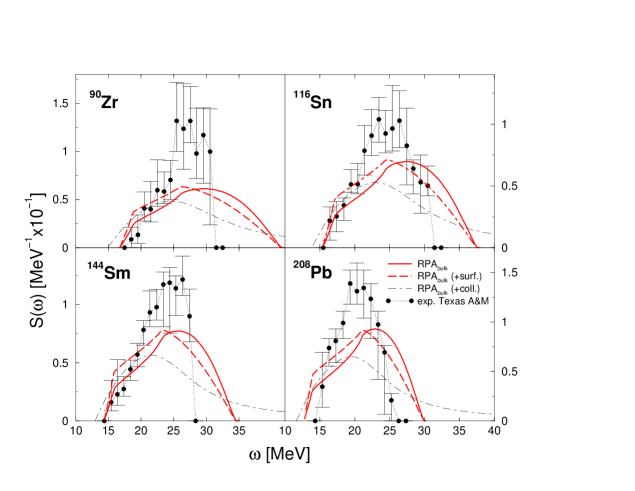
Fig. 1: The experimental structure function (T=0) versus theoretical values. The bulk RPA result (solid lines) is compared with the extended Thomas Fermi approximation (surface corrections, dashed lines) and the inclusion of collisions (dot-dashed lines). The latter one should be of less importance due to symmetry of isoscalar mode. The data suggest this case and support surface contributions. Circles: Normalized data from Ref.¹⁴⁾

After establishing the structure function including surface contribution we specify the model for actual calculations. We choose as mean field parameterization a Skyrme force following Vautherin and Brink⁹⁾ which leads to the isoscalar potential

$$V=\frac{3t_{0}}{4}+\frac{3t_{3}}{8}n_{0}$$ (17)

with $t_{0}=-983.4$ MeV fm³, $t_{3}=13106$ MeV fm⁶, $x_{0}=0.48$ at nuclear saturation density $n_{0}=0.16$ fm^-3 and the incompressibility of $K=318$ MeV. Further we employ the Steinwedel-Jensen model¹⁰⁾ where the basic mode inside a sphere of radius $R_{0}$ is given by a wave vector

$$q_{sp}={\pi\over 2R_{0}}.$$ (18)

This would correspond to the first order isovector mode¹¹⁾. Since this mode is spurious¹²⁾ we have to consider the next higher harmonics¹³⁾ which is

$$q_{isgdr}={\pi\over R_{0}}.$$ (19)

Since the polarization function with this second order mode contains still contributions from the spurious mode we have to subtract this part³⁾⁴⁾

$$\Pi^{0}_{\rm ISGDR}(\omega)=\Pi^{0}(q_{isgdr},\omega)-\Pi^{0}(q_{sp},\omega).$$ (20)

In Fig.1 we have plotted the experimental structure function together with different theoretical estimates according to (20) and (15). The inclusion of surface corrections (dashed lines) shifts the structure function towards the experimental values. The inclusion of collisions (dot-dashed lines), which should be of minor importance for isoscalar dipole mode due to cancellation of backscattering, leads to worse results. The results support also that the mode is of isoscalar dipole type.

References

1) M. N. Harakeh and A. E. L. Dieperink: Phys. Rev. C 23, 2329 (1981).

2) B. F. Davis et al.: Phys. Rev. Lett. 79, 609 (1997).

3) T. J. Deal: Nucl. Phys. A217, 210 (1973).

4) I. Hamamoto, H. Sagawa, and X. Z. Zhang: Phys. Rev. C 57, R1064 (1998).

5) N. V. Gai and H. Sagawa: Nucl. Phys. A371, 1 (1981).

6) P. Ring and P. Schuck: The Nuclear Many-Body Problem (Springer-Verlag, New York, 1980).

7) G. F. Bertsch and R. A. Broglia: Oscillations in Finite Quantum Systems (Cambridge Mongraphs, New York, 1994).

8) U. Kreibig and M. Vollmer: Optical Properties of Metal Cluster (Springer-Verlag, Berlin, 1995).

9) D. Vautherin and D. M. Brink: Phys. Rev. C 5, 626 (1972).

10) H. Steinwedel and J. Jensen: Z. f. Naturforschung 5, 413 (1950).

11) F. Braghin and D. Vautherin: Phys. Lett. B 333, 289 (1994).

12) K. Morawetz, R. Walke, and U. Fuhrmann: Phys. Rev. C 58, 1473 (1998).

13) K. Morawetz, U. Fuhrmann, and R. Walke: Nucl. Phys. A649, 348 (1999).

14) U. Garg: private communication.