Flavor content of nucleon form factors

Abstract

The flavor content of nucleon form factors is analyzed using two different theoretical approaches. The first is based on a phenomenological two-component model in which the external photon couples to both an intrinsic three-quark structure and a meson cloud via vector-meson dominance. The flavor content of the nucleon form factors is extracted without introducing any additional parameter. A comparison with recent data from parity-violating electron scattering experiments shows a good overall agreement for the strange form factors.

A more microscopic approach is that of an unquenched quark model proposed by Geiger and Isgur which is based on valence quark plus glue dominance to which quark-antiquark pairs are added in perturbation. In the original version the importance of $s\bar{s}$ loops in the proton was studied. Here we present the formalism for a new generation of unquenched quark models which, among other extensions, includes the contributions of $u\bar{u}$ and $d\bar{d}$ loops. Finally, we discuss some preliminary results in the closure limit.

Keywords: Baryons, strange form factors, vector meson dominance, quark models.

Se analiza el contenido de extrañeza de los factores de forma del nucleón usando dos métodos teóricos distintos. El primero está basado en un modelo fenomenológico de dos componentes en que el fotón se acopla tanto a una estructura intrínseca de tres cuarks como a una nube mesónica a través de la dominancia de mesones vectoriales. Se determina el contenido de sabor de los factores de forma del nucleón sin la necesidad de introducir algún parámetro adicional. Una comparación con datos recientes de experimentos de dispersión de electrones con violación de paridad muestra un buen ajuste para los factores de forma con extrañeza.

Un método más microscópico es el de un modelo de cuarks ’unquenched’ propuesto por Geiger e Isgur con base en la dominancia de cuarks de valencia más gluones al cual se agregan pares de cuark-anticuark en perturbación. En la versión original se estudió la importancia de los lazos $s\bar{s}$ para el protón. En este trabajo se presenta el formalismo de una nueva generación de modelos de cuarks ’unquenched’ que, entre otras extensiones, incluye las contribuciones de los lazos $u\bar{u}$ y $d\bar{d}$. Finalmente, se discuten algunos resultados preliminares en el límite de cerradura.

Descriptores: Bariones, factores de forma extraños, dominancia de mesones vectoriales, modelos de cuarks.

I Introduction

Recent experimental developments have made it possible to determine the flavor content of nucleon form factors. In particular the strange form factors of the proton can be obtained by combining asymmetry measurements in parity-violating electron scattering (PVES) Spayde ; Maas ; Happex ; Armstrong with either the electromagnetic form factors of the nucleon or with neutrino-proton scattering data Pate . The first results from the SAMPLE, PVA4, HAPPEX and G0 collaborations have shown evidence for a nonvanishing strange quark contribution, albeit small, to the charge and magnetization distributions of the proton Young .

In the constituent quark model (CQM), the proton is described in terms of a $uud$ three-quark configuration. Therefore, nonvanishing strange form factors provide direct evidence for the presence of higher Fock components in the proton wave function (such as $uud-s\bar{s}$ configurations). The contribution of strange quarks to the nucleon is of special interest because it is exclusively part of the quark-antiquark sea. There is a wide variety of CQMs: e.g. the Isgur-Karl model IK , the Capstick-Isgur model capstick , the algebraic $U(7)$ model bil1 ; bil2 , the hypercentral model pl , the chiral boson exchange model olof and the Bonn instanton model bn . Any of these models is able to reproduce the mass spectrum of baryon resonances reasonably well, but all of them show very similar deviations for other properties, such as for example the electromagnetic and strong decay widths of $\Delta(1232)$ and $N(1440)$, the spin-orbit splitting of $\Lambda(1405)$ and $\Lambda(1520)$, the transition form factors of $\Delta(1232)$, $N(1440)$, $N(1520)$, $N(1535)$ and $N(1680)$, and the large $\eta$ decay widths of the $N(1535)$, $\Lambda(1670)$ and $\Sigma(1750)$ resonances which are very close to the threshold for $\eta$ decay. In bil2 it was found that the main discrepancies occur for the low-lying $S$-wave states, specifically $N(1535)$, $\Lambda(1405)$, $\Lambda(1670)$, $\Lambda(1800)$ and $\Sigma(1750)$, which have masses close to the threshold of a meson-baryon decay channel. All of these results point towards the need to include exotic degrees of freedom (i.e. other than $qqq$), such as multiquark $q^{4}\bar{q}$ or gluonic $q^{3}g$ configurations. Another piece of evidence for quark-antiquark components in the proton comes from measurements of the $\bar{d}/\bar{u}$ asymmetry in the nucleon sea sea .

The role of higher Fock components in the CQM has been studied theoretically in a series of papers by Riska et al. riska in which it was shown that an appropriate admixture of some $q^{4}\bar{q}$ configurations may reduce the observed discrepancies between experiment and theory for several low-lying baryon resonances. In another CQM based approach by Isgur and collaborators, the effects of quark-antiquark pairs were included in a flux-tube breaking model based on valence-quark plus glue dominance to which $q\bar{q}$ pairs are added in perturbation mesons ; baryons . It was found necessary to sum over a large set of intermediate states in order to preserve the successes of the CQM, such as for example the OZI hierarchy OZI . In deMelo , a possible change of sign in the proton form factor ratio $\mu_{p}G_{E}^{p}/G_{M}^{p}$ is attributed to the interplay between the contribution from the elastic quark-photon vertex and the one from the pair production process, i.e. higher Fock components.

The aim of the present contribution is to study the importance of quark-antiquark pairs in baryon spectroscopy. We start by analyzing the available experimental data on strange form factors in a phenomenological approach RB1 based on a two-component model of nucleon form factors in terms of an intrinsic structure ($qqq$ configuration) surrounded by a meson cloud ($q\bar{q}$ pairs) BI from which the flavor content is extracted according to a procedure first introduced by Jaffe Jaffe . Next we present an unquenched quark model which is a generalization of the flux-tube breaking model proposed by Geiger and Isgur baryons . As a first application, we discuss the flavor decomposition of the spin of the ground state octet and decuplet baryons in the closure limit.

II Two-component model

First we study the strange form factors of the nucleon in a phenomenological two-component model IJL ; BI in which it is assumed that the external photon couples both to an intrinsic three-quark structure described by the dipole form factor $g(Q^{2})=1/(1+\gamma Q^{2})^{2}$, and to a meson cloud via vector-meson ($\rho$, $\omega$ and $\phi$) dominance (VMD). In the original VMD calculation IJL , the Dirac form factor was attributed to both the intrinsic structure and the meson cloud, and the Pauli form factor entirely to the meson cloud. In BI , it was shown that the addition of an intrinsic part to the isovector Pauli form factor, as suggested by studies of relativistic constituent quark models in the light-front approach frank , considerably improves the results for the neutron electric and magnetic form factors.

II.1 Strange form factors

Electromagnetic and weak form factors contain the information about the distribution of electric charge and magnetization inside the nucleon. These form factors arise from matrix elements of the corresponding vector current operators

$$\left<N\left|V_{\mu}\right|N\right>=\bar{u}_{N}\left[F_{1}(Q^{2})\,\gamma_{\mu}+\frac{i}{2M_{N}}F_{2}(Q^{2})\,\sigma_{\mu\nu}q^{\nu}\right]u_{N}~{}.$$ (1)

Here $F_{1}$ and $F_{2}$ are the Dirac and Pauli form factors, which are functions of the squared momentum transfer $Q^{2}=-q^{2}$. The electric and magnetic form factors, $G_{E}$ and $G_{M}$, are obtained from $F_{1}$ and $F_{2}$ by the relations $G_{E}=F_{1}-\tau F_{2}$ and $G_{M}=F_{1}+F_{2}$ with $\tau=Q^{2}/4M_{N}^{2}$.

Since the intrinsic part is associated with the valence quarks of the nucleon, the strange quark content of the nucleon form factors arises from the (isoscalar) meson wave functions

$$\left|\omega\right> = \cos\epsilon\left|\omega_{0}\right>-\sin\epsilon\left|\phi_{0}\right>,$$

$$\left|\phi\right> = \sin\epsilon\left|\omega_{0}\right>+\cos\epsilon\left|\phi_{0}\right>,$$ (2)

where $\left|\omega_{0}\right>=\left(u\bar{u}+d\bar{d}\right)/\sqrt{2}$ and $\left|\phi_{0}\right>=s\bar{s}$ are the ideally mixed states. Under the assumption that the strange form factors have the same form as the isoscalar ones, the strange Dirac and Pauli form factors are expressed as the product of an intrinsic part $g(Q^{2})$ and a contribution from the meson cloud as RB1

$$F_{1}^{s}(Q^{2}) = \frac{1}{2}g(Q^{2})\left[\beta_{\omega}^{s}\frac{m_{\omega}^{2}}{m_{\omega}^{2}+Q^{2}}+\beta_{\phi}^{s}\frac{m_{\phi}^{2}}{m_{\phi}^{2}+Q^{2}}\right]~{},$$

$$F_{2}^{s}(Q^{2}) = \frac{1}{2}g(Q^{2})\left[\alpha_{\omega}^{s}\frac{m_{\omega}^{2}}{m_{\omega}^{2}+Q^{2}}+\alpha_{\phi}^{s}\frac{m_{\phi}^{2}}{m_{\phi}^{2}+Q^{2}}\right]~{},$$ (3)

where the $\beta$’s and $\alpha$’s are related to the two independent isoscalar couplings $\beta_{\omega}$ and $\alpha_{\phi}$ RB1 ; RB2

$$\beta_{\omega}^{s} = -\beta_{\phi}^{s}=-\sqrt{6}\,\frac{\sin\epsilon}{\sin(\theta_{0}+\epsilon)}\beta_{\omega}~{},$$

$$\alpha_{\omega}^{s} = -\sqrt{6}\,\frac{\sin\epsilon}{\sin(\theta_{0}+\epsilon)}\left(\mu_{p}+\mu_{n}-1-\alpha_{\phi}\right)~{},$$

$$\alpha_{\phi}^{s} = -\sqrt{6}\,\frac{\cos\epsilon}{\cos(\theta_{0}+\epsilon)}\alpha_{\phi}~{}.$$ (4)

Here $\tan\theta_{0}=1/\sqrt{2}$. The Dirac form factor $F_{1}^{s}$ is small due to canceling contributions of the $\omega$ and $\phi$ couplings which arise as a consequence of the fact that the strange (anti)quarks do not contribute to the electric charge $G_{E}^{s}(0)=F_{1}^{s}(0)=\beta_{\omega}^{s}+\beta_{\phi}^{s}=0$.

The mixing angle $\epsilon$ can be determined from the decay properties of the $\omega$ and $\phi$ mesons as $\epsilon=0.053$ rad Jain . Since the mixing angle is very small, it is worth examining the results for the strange Dirac and Pauli form factors in the absence of mixing. In the limit of zero mixing, the strangeness contribution arises entire from the Pauli coupling of the $\phi$ meson $\alpha^{s}_{\phi}$

$$F_{1}^{s}(Q^{2}) \rightarrow 0~{},$$

$$F_{2}^{s}(Q^{2}) \rightarrow \frac{1}{2}g(Q^{2})\,\alpha_{\phi}^{s}\frac{m_{\phi}^{2}}{m_{\phi}^{2}+Q^{2}}~{}.$$ (5)

II.2 Results

In the present calculation of the strange form factors, the coefficient $\gamma$ in the intrinsic form factor and the isoscalar couplings, $\beta_{\omega}$ and $\alpha_{\phi}$, are taken from a study of the electromagnetic form factors of the nucleon. According to Eq. (4), the strange couplings can be determined from the isoscalar couplings: $\beta_{\phi}^{s}=-\beta_{\omega}^{s}=0.202$, $\alpha_{\phi}^{s}=0.648$ and $\alpha_{\omega}^{s}=-0.018$ RB1 .

Figs. 1 and 2 show the strange electric and magnetic form factors as a function of $Q^{2}$. The qualitative features can be understood in the limit of ideally mixed mesons, i.e. zero mixing angle (in comparison with the value of $\epsilon=3.0^{\circ}$ used in Figs. 1 and 2). In this case, according to Eq. (5) the Dirac form factor vanishes. Hence the strange electric and magnetic form factors reduce to

$$G_{E}^{s} \rightarrow -\tau F_{2}^{s}~{},$$

$$G_{M}^{s} \rightarrow F_{2}^{s}~{}.$$ (6)

The strange electric form factor is small since, for the range of $Q^{2}$ in Fig. 1, the contribution from the Pauli form factor is suppressed by the factor $\tau=Q^{2}/4M_{N}^{2}$.

The theoretical values are in good agreement with the recent experimental results of the HAPPEX Collaboration in which $G_{E}^{s}$ was determined in PVES from a ⁴He target Happex , as well as with the result from an analysis of the world data $G_{E}^{s}(Q^{2}=0.1)=-0.005\pm 0.019$ Happex and from a lattice QCD calculation $G_{E}^{s}(0.1)=-0.009\pm 0.005\pm 0.003\pm 0.027$ leinweber2 .

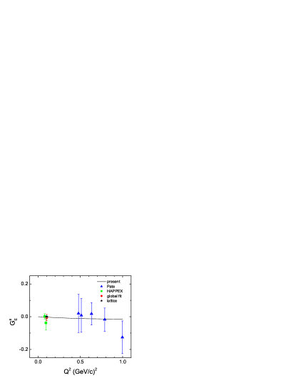
Figure 1: Comparison between theoretical and experimental values of the strange electric form factor. The experimental values are taken from Happex (squares), a global fit Happex (circle) and Pate (triangles). The result from lattice QCD is indicated by a star leinweber2 .

The strange magnetic form factor $G_{M}^{s}=F_{1}^{s}+F_{2}^{s}$ is positive, since it is dominated by the contribution from the Pauli form factor. The SAMPLE experiment measured the parity-violating asymmetry at backward angles, which allowed the strange magnetic form factor at $Q^{2}=0.1$ (GeV/c)² to be determined as $G_{M}^{s}=0.37\pm 0.20\pm 0.26\pm 0.07$. An analysis of the world data at the same value of $Q^{2}$ gives $G_{M}^{s}=0.18\pm 0.27$ Happex . The other experimental values of $G_{E}^{s}$ and $G_{M}^{s}$ in Figs. 1 and 2 were obtained Pate by combining the (anti)neutrino data from E734 Ahrens with the parity-violating asymmetries from HAPPEX Happex and G0 Armstrong . The theoretical values are in good overall agreement with the experimental ones for the entire range $0<Q^{2}<1.0$ (GeV/c)².

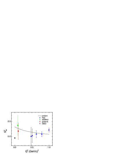
Figure 2: Comparison between theoretical and experimental values of the strange magnetic form factor. The experimental values are taken from Spayde (square), a global fit Happex (circle) and Pate (triangles). The result from lattice QCD is indicated by a star leinweber1 .

The strange magnetic moment is calculated to be positive

$$\mu_{s}=G_{M}^{s}(0)=\frac{1}{2}(\alpha_{\omega}^{s}+\alpha_{\phi}^{s})=0.315\,\mu_{N}~{},$$ (7)

in units of the nuclear magneton, $\mu_{N}=e\hbar/2M_{N}c$. This value is in agreement with that of a recent analysis of the world data on strange form factors in the range of $0<Q^{2}<3$ (GeV/c)² which gives $\mu_{s}=0.37\pm 0.79$ $\mu_{N}$ Young . We note that the latter evaluation did not include the new HAPPEX data from Happex . Theoretical calculations of the strange magnetic moment show a large variation, although most QCD-inspired models seem to favor a negative value in the range $-0.6\lesssim\mu_{s}\lesssim 0.0$ $\mu_{N}$ beck . Recent lattice-QCD calculations give small values, e.g. $0.05\pm 0.06$ lewis and $-0.046\pm 0.019$ leinweber1 .

Most experimental data on strange form factors correspond to a linear combination of electric and magnetic form factors $G_{E}^{s}+\eta G_{M}^{s}$. In RB1 ; RB2 it was shown that the calculated values in the two-component model are in good overall agreement with the experimental data from the PVA4 Maas , HAPPEX Happex and G0 collaborations Armstrong . Finally, a flavor decomposition of the nucleon electromagnetic form factors shows that the contribution of the strange quarks to the proton form factors is small, being of the order of a few percent of the total RB2 .

Another recent extension of the two-component model of the nucleon has been to the transition form factors of baryon resonances Wan . The two-component model has the disadvantage that its applicability depends on the availability of a good and reliable set of experimental data to be able to determine the coefficients in the Dirac and Pauli form factors. The couplings between the intrinsic structure and the quark-antiquark pairs are obtained in a phenomenological rather than a dynamical way, in which these couplings would be the result of a specific interaction term. In the next section, we discuss the flux-tube breaking model, in which the effects of the higher Fock components are included via a ${}^{3}P_{0}$ coupling mechanism.

III Flux-tube breaking model

In the flux-tube model for hadrons, the quark potential model arises from an adiabatic approximation to the gluonic degrees of freedom embodied in the flux tube flux . The impact of quark-antiquark pairs in meson spectroscopy has been studied in an elementary flux-tube breaking model mesons in which the $q\bar{q}$ pair is created with the ${}^{3}P_{0}$ quantum numbers of the vacuum. Subsequently, it was shown by Geiger and Isgur OZI that a "miraculous" set of cancellations between apparently uncorrelated sets of intermediate states occurs in such a way that they compensate each other and do not destroy the good CQM results for the mesons. In particular, the OZI hierarchy is preserved and there is a near immunity of the long-range confining potential, since the change in the linear potential due to the creation of quark-antiquark pairs in the string can be reabsorbed into a new strength of the linear potential, i.e. in a new string tension. As a result, the net effect of the mass shifts from pair creation is smaller than the naive expectation of the order of the strong decay widths. However, it is necessary to sum over large towers of intermediate states to see that the spectrum of the mesons, after unquenching and renormalizing, is only weakly perturbed. An important conclusion is that no simple truncation of the set of meson loops is able to reproduce such results OZI .

Figure 3: Quark line diagrams for $A\rightarrow BC$ with $q_{1}q_{2}q_{3}=uud$ and $q\bar{q}=s\bar{s}$

The extension of the flux-tube breaking model to baryons requires a proper treatment of the permutation symmetry between identical quarks. As a first step, Geiger and Isgur investigated the importance of $s\bar{s}$ loops in the proton by taking into account the contribution of the six different diagrams of Fig. 3 with $q\bar{q}=s\bar{s}$ and $q_{1}q_{2}q_{3}=uud$, and by using harmonic oscillator wave functions for the baryons and mesons baryons . In the conclusions, the authors emphasized: It also seems very worthwhile to extend this calculation to $u\bar{u}$ and $d\bar{d}$ loops. Such an extension could reveal the origin of the observed violations of the Gottfried sum rule and also complete our understanding of the origin of the spin crisis. In this contribution, we take up this challenge and present the first results for some generalizations of the formalism of baryons which make it now possible to study the quark-antiquark contributions

• for any initial baryon resonance

• for any flavor of the quark-antiquark pair

• for any model of baryons and mesons, as long as their wave functions are expressed on the basis of the harmonic oscillator.

The problem of the permutation symmetry between identical quarks has been solved by means of group-theoretical techniques. In this way, the quark-antiquark contribution can be calculated for any initial baryon $q_{1}q_{2}q_{3}$ (ground state or resonance) and for any flavor of the quark-antiquark pair $q\bar{q}$ (not only $s\bar{s}$, but also $u\bar{u}$ and $d\bar{d}$).

Figure 4: One-loop diagram

Here we adopt the unquenched quark model of baryons , which is based on an adiabatic treatment of the flux-tube dynamics to which the $q\bar{q}$ pair creation with vacuum quantum numbers is added as a perturbation. The pair-creation mechanism is inserted at the quark level and the one-loop diagrams are calculated by summing over a complete set of intermediate states (see Fig. 4). Under these assumptions, the baryon wave function is, to leading order in pair creation, given by

$$\mid\psi_{A}\rangle\;=\;{\cal N}\left[\mid A\rangle+\sum_{qBClJ}\int d\vec{k}\,\mid BC\vec{k}\,lJ\rangle\,\frac{\langle BC\vec{k}\,lJ\mid h_{q\bar{q}}^{\dagger}\mid A\rangle}{M_{A}-E_{B}-E_{C}}\right]~{},$$ (8)

where $h_{q\bar{q}}^{\dagger}$ is the ${}^{3}P_{0}$ quark-antiquark pair-creation operator baryons , $A$ is the initial baryon, $B$ and $C$ denote the intermediate baryon and meson, $\vec{k}$ and $l$ the relative radial momentum and orbital angular momentum of $B$ and $C$, and $J$ is the total angular momentum $\vec{J}=\vec{J}_{BC}+\vec{l}=\vec{J}_{B}+\vec{J}_{C}+\vec{l}$. The sum over $q$ denotes the sum over all flavors of the $q\bar{q}$ pair.

In general, matrix elements of an observable $\hat{\cal O}$ can be expressed as

$${\cal O}\;=\;\langle\psi_{A}\mid\hat{\cal O}\mid\psi_{A}\rangle\;=\;{\cal O}_{\rm valence}+{\cal O}_{\rm sea}~{},$$ (9)

where the first term denotes the contribution from the valence quarks

$${\cal O}_{\rm valence} = {\cal N}^{2}\langle A\mid\hat{\cal O}\mid A\rangle$$ (10)

and the second term that from the quark-antiquark pairs

$${\cal O}_{\rm sea} = {\cal N}^{2}\sum_{qBClJ}\int d\vec{k}\,\sum_{q^{\prime}B^{\prime}C^{\prime}l^{\prime}J^{\prime}}\int d\vec{k}^{\,\prime}\,\frac{\langle A\mid h_{q^{\prime}\bar{q}^{\prime}}\mid B^{\prime}C^{\prime}\vec{k}^{\,\prime}\,l^{\prime}J^{\prime}\rangle}{M_{A}-E_{B^{\prime}}-E_{C^{\prime}}}$$ (11)

$$\hskip 56.9055pt\langle B^{\prime}C^{\prime}\vec{k}^{\,\prime}\,l^{\prime}J^{\prime}\mid\hat{\cal O}\mid BC\vec{k}\,lJ\rangle\,\frac{\langle BC\vec{k}\,lJ\mid h_{q\bar{q}}^{\dagger}\mid A\rangle}{M_{A}-E_{B}-E_{C}}~{}.$$

The sum in Eq. (11) is over a complete set of intermediate states, rather than just a few low-lying states. Not only does this have a significant impact on the numerical result, but it is necessary for consistency with the OZI-rule and the success of CQM’s in hadron spectroscopy. We have developed an algorithm based upon group-theoretical techniques to generate the intermediate states with the correct permutational symmetry for any model of hadrons. Therefore, the sum over intermediate states can be perfomed up to saturation, and not just for the first few shells as in baryons .

III.1 Closure limit

The evaluation of the contribution of the quark-antiquark pairs simplifies considerably in the closure limit, which arises when the energy denominators do not depend strongly on the quantum numbers of the intermediate states in Eq. (11). In this case, the sum over the complete set of intermediate states can be solved by closure and the contribution of the quark-antiquark pairs to the matrix element reduces to

$${\cal O}_{\rm sea} \propto \sum_{qq^{\prime}}\langle A\mid h_{q^{\prime}\bar{q}^{\prime}}\,\hat{\cal O}\,h_{q\bar{q}}^{\dagger}\mid A\rangle~{}.$$ (12)

Especially when combined with symmetries, the closure limit not only provides simple expressions for the relative flavor content of physical observables, but also can give further insight into the origin of cancellations between the contributions from different intermediate states.

Figure 5: Ground state decuplet baryons

As an example, we discuss some preliminary results for the operator

$$\Delta q\;=\;2\langle S_{z}(q)+S_{z}(\bar{q})\rangle~{},$$ (13)

which determines the fraction of the baryon’s spin carried by each one of the flavors $u$, $d$ and $s$. First, we consider the ground state decuplet baryons with ${}^{4}10[56,0^{+}]_{3/2}$ of Fig. 5. Since the three-quark configuration of the $\Delta$ resonances does not contain strange quarks, the contribution of the $s\bar{s}$ pairs to the spin $\Delta s$ vanishes in the closure limit. The same holds for the contribution of $d\bar{d}$ pairs to the $\Delta^{++}$, $\Sigma^{\ast\,+}$, $\Xi^{\ast\,0}$ and $\Omega^{-}$ resonances, and that of $u\bar{u}$ pairs to the $\Delta^{-}$, $\Sigma^{\ast\,-}$, $\Xi^{\ast\,-}$ and $\Omega^{-}$ resonances. Moreover, in the closure limit the relative contribution of the quark flavors from the quark-antiquark pairs to the baryon spin is the same as that from the valence quarks

$$\Delta u_{\rm sea}:\Delta d_{\rm sea}:\Delta s_{\rm sea}\;=\;\Delta u_{\rm valence}:\Delta d_{\rm valence}:\Delta s_{\rm valence}~{}.$$ (14)

This property is a consequence of the spin-flavor symmetry of the ground state baryons and holds for both the decuplet with quantum numbers ${}^{4}10[56,0^{+}]_{3/2}$ and the octet with ${}^{2}10[56,0^{+}]_{1/2}$. Table 1 shows the relative contributions of $\Delta u$, $\Delta d$ and $\Delta s$ to the spin of the ground state baryons in the closure limit. At a qualitative level, a vanishing closure limit explains the phenomenological success of CQMs. As an example, the strange content of the proton which vanishes in the closure limit is expected to be small, in agreement with the experimental data from PVES (for the most recent data see Happex ; Armstrong ). Moreover, the results in Table 1 impose very stringent conditions on the numerical calculations, since each entry involves the sum over a complete set of intermediate states. Therefore, the closure limit provides a highly nontrivial test which involves both the spin-flavor sector, the permutation symmetry, the construction of a complete set of intermediate states and the implementation of the sum over all of these states.

Table 1: Relative contributions of $\Delta u$, $\Delta d$ and $\Delta s$ in the closure limit to the spin of the ground state octet and decuplet baryons

$qqq$	${}^{2}8[56,0^{+}]$	$\Delta u$	:	$\Delta d$	:	$\Delta s$	${}^{4}10[56,0^{+}]$	$\Delta u$	:	$\Delta d$	:	$\Delta s$
$uuu$							$\Delta^{++}$	9	:	0	:	0
$uud$	$p$	4	:	$-1$	:	0	$\Delta^{+}$	6	:	3	:	0
$udd$	$n$	$-1$	:	4	:	0	$\Delta^{0}$	3	:	6	:	0
$ddd$							$\Delta^{-}$	0	:	9	:	0
$uus$	$\Sigma^{+}$	4	:	0	:	$-1$	$\Sigma^{\ast\,+}$	6	:	0	:	3
$uds$	$\Sigma^{0}$	2	:	2	:	$-1$	$\Sigma^{\ast\,0}$	3	:	3	:	3
	$\Lambda$	0	:	0	:	3
$dds$	$\Sigma^{-}$	0	:	4	:	$-1$	$\Sigma^{\ast\,-}$	0	:	6	:	3
$uss$	$\Xi^{0}$	$-1$	:	0	:	4	$\Xi^{\ast\,0}$	3	:	0	:	6
$dss$	$\Xi^{-}$	0	:	$-1$	:	4	$\Xi^{\ast\,-}$	0	:	3	:	6
$sss$							$\Omega^{-}$	0	:	0	:	9

IV Summary, conclusions and outlook

In summary, we have discussed the importance of quark-antiquark pairs in baryon spectroscopy. A direct handle on these higher Fock components is provided by PVES experiments, which have shown evidence for a nonvanishing strange quark contribution, albeit small, to the charge and magnetization distributions of the proton.

In the first part of this contribution, we reviewed an analysis of the recent data on strange form factors in a phenomenological two-component model which consists of an intrinsic (valence quark) structure surrounded by a meson cloud (quark-antiquark pairs) RB1 . It is important to note that the flavor content of the nucleon form factors is extracted without introducing any additional parameter. All couplings were determined from a previous study of a simultaneous fit to the electromagnetic form factors of the nucleon (as a matter of fact, the static condition on the strange electric form factor $G_{E}^{s}(0)=0$ puts an additional constraint on the parameters, thus effectively reducing the number of independent parameters by one RB1 ). A comparison with recent data from PVES experiments shows a good overall agreement for both the strange electric and magnetic form factors for the range of $0<Q^{2}<1$ (GeV/c)². Therefore, one may conclude that the two-component model provides a simultaneous and consistent description of the electromagnetic and weak vector form factors of the nucleon. Future experiments on parity-violating electron scattering at backward angles (PVA4 and G0 g0back ) and neutrino scattering (FINeSSE finesse ) will make it possible to disentangle the contributions of the different quark flavors to the electric, magnetic and axial form factors, and thus to gain new insight into the complex internal structure of the nucleon.

In the second part, we discussed the first results from a more microscopic approach to include the effects of the quark-antiquark pairs. The method is based on the dominance of valence quarks and gluon dynamics to which the $q\bar{q}$ pairs are added as a perturbation. The ensuing flux-tube breaking model was originally introduced by Kokoski and Isgur for mesons mesons and later extended by Geiger and Isgur to $s\bar{s}$ loops in the proton baryons . In this contribution, we presented a new generation of unquenched quark models for baryons by including, in addition to $s\bar{s}$ loops, the contributions of $u\bar{u}$ and $d\bar{d}$ loops as well. As an illustration, we applied the closure limit of the model - in which all intermediate states are assumed to be degenerate - to the flavor decomposition of the spin of the ground state octet and decuplet baryons. In this case, it was found that the relative contributions of the quark flavors from the $q\bar{q}$ pairs are the same as that from the valence quarks.

The present formalism is, obviously within the assumptions of the approach, valid for any initial baryon, any flavor of the $q\bar{q}$ pairs and any model of hadron structure. In future work, it will be applied systematically to study several problems in light baryon spectroscopy, such as the spin crisis of the proton, the electromagnetic and strong couplings, the electromagnetic elastic and transition form factors of baryon resonances, their sea quark content and their flavor decomposition new .

References

-
(1)
D.T. Spayde et al., Phys. Lett. B 583, 79 (2004);
E.J. Beise, M.L. Pitt and D.T. Spayde, Prog. Part. Nucl. Phys. 54, 289 (2005). - (2) F.E. Maas et al., Phys. Rev. Lett. 93, 022002 (2004); ibid., 94, 152001 (2005).
-
(3)
K.A. Aniol et al., Phys. Rev. C 69, 065501 (2004);
K.A. Aniol et al., Phys. Lett. B 635, 275 (2006);
K.A. Aniol et al., Phys. Rev. Lett. 96, 022003 (2006);
A. Acha et al., Phys. Rev. Lett. 98, 032301 (2007). - (4) D.S. Armstrong et al., Phys. Rev. Lett. 95, 092001 (2005).
-
(5)
S.F. Pate, Phys. Rev. Lett. 92, 082002 (2004);
S.F. Pate, G. MacLachlan, D. McKee and V. Papavassiliou, AIP Conf. Proc. 842, 309 (2006). - (6) R.D. Young, J. Roche, R.D. Carlini and A.W. Thomas, Phys. Rev. Lett. 97, 102002 (2006).
- (7) N. Isgur and G. Karl, Phys. Rev. D 20, 1191 (1979).
- (8) S. Capstick and N. Isgur, Phys. Rev. D 34, 2809 (1986).
-
(9)
R. Bijker, F. Iachello and A. Leviatan,
Ann. Phys. (N.Y.) 236, 69 (1994);
R. Bijker, F. Iachello and A. Leviatan, Phys. Rev. C 54, 1935 (1996). - (10) R. Bijker, F. Iachello and A. Leviatan, Ann. Phys. (N.Y.) 284, 89 (2000).
-
(11)
M. Ferraris, M.M. Giannini, M. Pizzo, E. Santopinto and L. Tiator,
Phys. Lett. B 364, 231 (1995);
M. Aiello, M. Ferraris, M.M. Giannini, M. Pizzo and E. Santopinto, Phys. Lett. B 387, 215 (1996);
M. Aiello, M.M. Giannini and E. Santopinto, J. Phys. G: Nucl. Part. Phys. 24, 753 (1998). -
(12)
L.Ya. Glozman and D.O. Riska,
Phys. Rep. 268, 263 (1996);
L.Ya. Glozman, Z. Papp, W. Plessas, K. Varga and R.F. Wagenbrunn, Phys. Rev. C 57, 3406 (1998);
L.Ya. Glozman, W. Plessas, K. Varga and R.F. Wagenbrunn, Phys. Rev. D 58, 094030 (1998). -
(13)
U. Löring, K. Kretzschmar, B.Ch. Metsch, H.R. Petry,
Eur. Phys. J. A 10, 309 (2001);
U. Löring, B.Ch. Metsch, H.R. Petry, Eur. Phys. J. A 10, 395 (2001); ibid. 10, 447 (2001). - (14) G.T. Garvey and J.-C. Peng, Progr. Part. Nucl. Phys. 47, 203 (2001).
-
(15)
C. Helminen and D.O. Riska, Nucl. Phys. A 699, 624 (2002);
Q.B. Li and D.O. Riska, Nucl. Phys. A 766, 172 (2006);
B. Juliá-Díaz and D.O. Riska, Nucl. Phys. A 780, 175 (2006);
Q.B. Li and D.O. Riska, Phys. Rev. C 73, 035201 (2006); ibid. 74, 015202 (2006);
Q.B. Li and D.O. Riska, arXiv:nucl-th/0702049. - (16) R. Kokoski and N. Isgur, Phys. Rev. D 35, 907 (1987).
- (17) P. Geiger and N. Isgur, Phys. Rev. D 55, 299 (1997).
-
(18)
P. Geiger and N. Isgur,
Phys. Rev. Lett. 67, 1066 (1991);
P. Geiger and N. Isgur, Phys. Rev. D 44, 799 (1991); ibid. 47, 5050 (1993). - (19) J.P.B.C. de Melo, T. Frederico, E. Pace, S. Pisano and G. Salmè, Nucl. Phys. A 782, 69c (2007).
- (20) R. Bijker, J. Phys. G: Nucl. Part. Phys. 32, L49 (2006) [arXiv:nucl-th/0511060].
- (21) R. Bijker and F. Iachello, Phys. Rev. C 69, 068201 (2004).
- (22) R.L. Jaffe, Phys. Lett. B 229, 275 (1989).
- (23) F. Iachello, A.D. Jackson and A. Lande, Phys. Lett. B 43, 191 (1973).
-
(24)
M.R. Frank, B.K. Jennings and G.A. Miller,
Phys. Rev. C 54, 920 (1996);
E. Pace, G. Salmè, F. Cardarelli and S. Simula, Nucl. Phys. A 666, 33c (2000). -
(25)
R. Bijker, Eur. Phys. J. A, in press [arXiv:nucl-th/0607058];
R. Bijker, Rev. Mex. Fís. S 52 (4), 1 (2006). - (26) P. Jain, R. Johnson, U.-G. Meissner, N.W. Park and J. Schechter, Phys. Rev. D 37, 3252 (1988).
- (27) D.B. Leinweber, S. Boinepalli, A.W. Thomas, P. Wang, A.G. Williams, R.D. Young, J.M. Zanotti and J.B. Zhang, Phys. Rev. Lett. 97, 022001 (2006).
- (28) L.A. Ahrens et al., Phys. Rev. D 35, 785 (1987).
-
(29)
K.S. Kumar and P.A. Souder,
Progr. Part. Nucl. Phys. 45, S333 (2000);
D.H. Beck and B.R. Holstein, Int. J. Mod. Phys. E 10, 1 (2001);
D.H. Beck and R.D. McKeown, Annu. Rev. Nucl. Part. Sci. 51, 189 (2001). - (30) R. Lewis, W. Wilcox and R.M. Woloshyn, Phys. Rev. D 67, 013003 (2003).
- (31) D.B. Leinweber, S. Boinepalli, I.C. Cloet, A.W. Thomas, A.G. Williams, R.D. Young, J.M. Zanotti and J.B. Zhang, Phys. Rev. Lett. 94, 212001 (2005).
-
(32)
Q. Wan and F. Iachello, Int. J. Mod. Phys. A 20, 1846 (2005);
Q. Wan, Ph.D. Thesis, Yale University, 2006. - (33) N. Isgur and J. Paton, Phys. Rev. D 31, 2910 (1985).
- (34) D.H. Beck, JLab Experiment E-04-115.
- (35) B.T. Fleming and R. Tayloe, FINeSSE proposal, arXiv:hep-ex/0502014.
- (36) R. Bijker and E. Santopinto, work in progress.