Initial Parton Distribution just after Heavy Ion Collisions

Abstract

We study the initial distribution of a parton system which is formed just after relativistic heavy ion collision by the elastic scattering among the constituent partons in details and analyze the baryon and strangeness contents of the primary parton system. We present the rapidity and energy distributions of the system.

I Introduction

The relativistic heavy ion collision at RHIC or LHC energy liberates lots of constituent partons of nuclei by primary collisions and those partons evolve according to quantum theory and may become a quark-gluon plasma which has been searched intensively by AGS and RHIC. The study of the early system of those partons thus are very important and we somehow have to know the momentum distribution as well as the space distribution to understand in details the dynamics of the system as a function of time.

There are several schemes to obtain the initial (phase space) distribution of partons: The constituent partons of a nucleus can be characterized by the Feynman x where the soft parton has small x and the hard one large x. The soft parton can be identified as the non-abelian Weizsacker-Williams field radiated from the hard partons and is dominant in number. While the two nuclei pass through each other in collision, the high x partons of one nucleus can be scattered off from those high x partons of the other nucleus and the non-abelian Weicsacker-Williams field lose the coherence of the parent parton and become particles. This initial parton information has been studied by Krasnitz et alknv03 and Lappilap03 based on CGCmcl94 ; am00 , namely, shattering of the color glass condensates of two colliding nuclei, and the analytic distribution function has been proposed. It however can be applicable to the central rapidity region only and the production of quarks or antiquarks can not be calculated from the scheme.

Another theory to produce dynamically the partons after a heavy ion collision is that while the colliding nuclei is passing through each other, they rapidly decelerate and produce Schwinger-like radiation already in thermal spectrumkha06 . The background field are the pulse-like CGC of McLerran-Venugopalan model of the other nucleus. This theory could provide the scenario to explain the fast thermalization of the parton system.

Even though we can understand the gluon production from these studies, those do not provide the initial baryon density which is shown in RHIC experimentsstar05 ; phen05 . To understand this phenomena we certainly have to include quarks as well as antiquarks from the primary collision. Consider the CM frame of two colliding nuclei at high energy. The colliding nuclei are Lorentz contracted to become disks and the transversal motion of constituent partons can be ignored since the longitudinal momentum is dominant at high energy. When the colliding nuclei pass through each other, the constituents of a projectile nucleus make scattering with those of a target nucleus(note that the partons in the same nucleus do not collide with each other since the time delation) and become particles if the momentum transfer is large enough. This, so-called, factorization method, has been used to calculate jets or minijetseks96 ; nayak ; ham99 ; coo02 from early 80s. There are many schemes to obtain the parton distribution of a hadron or a nucleusszc : for examples, we can fold the parton distribution of a nucleon and the nucleon distribution of a nucleusgrv98 ; eks99 . The wave function of a high energy nucleus has been studied extensively and we use GRV98, CTEQ and an emperical distribution in our study. Since this method only gives relatively high $p_{\perp}$ partons but soft partons can not be obtained so that it gives a reasonable distribution at higher energy but does not give good at RHIC energy. The studies on this direction had been persuited by Eskolaeks96 , by Hammon et al.ham99 , by Nayak et al.nayak and by Cooper et al.coo02 . We however think it is worth to extend the study to include baryon and strangeness contents at RHIC and LHC energy. We also briefly note here that the spatial distribution of produced partons can be understood assuming that the quanta becomes particle after the time $1/E_{T}$, which $E_{T}$ is the transversal energy of the quanta and at the place where the quanta travels ${\vec{p}}/EE_{T}$ from the scattering point.

We rewrite the basic formulas to calculate the production of partons in Section II. We present the numerical results in Section III. We summarize and conclude in Section IV.

II Initial parton production

We assume that partons are produced at relativistic heavy-ion collisions by elastic scattering between the constituent of a projectile nucleus and that of a target nucleus. Since the scattering cross section gives the number of collision events per unit overlap area, we can write the total number of events eks96 ; ham99 ; coo02 ; book :

$${N^{event}} = KT(b)\int dy_{3}dy_{4}d^{2}p_{T}\sum_{ij,\,kl}x_{1}f_{i/A}(x_{1},Q_{0}^{2})x_{2}f_{j/B}(x_{2},Q_{0}^{2}){{d\sigma^{ij\rightarrow kl}(\hat{s},\hat{t},\hat{u})}\over{d{\hat{t}}}},$$ (1)

where a parton $i$ of the nucleus $A$ makes a collision with a parton $j$ of the nucleus $B$ and produces partons $k$ and $l$. Each parton has rapidity $y_{1}$, $y_{2}$, $y_{3}$ and $y_{4}$, respectively. $x_{1}$ and $x_{2}$ are the Bjorken scaling variables of parton $i$ and $j$. The relations between the variables before and after the collision are given by

$$x_{1} = p_{T}(e^{y_{1}}+e^{y_{2}})/\sqrt{s},$$ (2)

$$x_{2} = p_{T}(e^{-y_{1}}+e^{-y_{2}})/\sqrt{s},$$ (3)

$$\hat{s} = x_{1}x_{2}s,$$ (4)

$$\hat{t} = -p_{T}^{2}(1+e^{y_{2}-y_{1}}),$$ (5)

$$\hat{u} = -p_{T}^{2}(1+e^{y_{1}-y_{2}}).$$ (6)

We also rewrite the available kinematic region for convenience ham99 ; shin02 ; shin03 ,

$$Q_{0}\,^{2}\leq p_{T}\,^{2}\leq({{\sqrt{s}}\over{2\cosh y}})^{2},$$ (7)

$$-\log({{\sqrt{s}}\over{p_{T}}}-e^{-y})\leq y_{4}\leq\log({{\sqrt{s}}\over{p_{T}}}-e^{-y}),$$ (8)

$$|y|\leq\log({{\sqrt{s}}\over{2Q_{0}}}+\sqrt{{{s}\over{4Q_{0}\,^{2}}}-1}).$$ (9)

$K$ is the K-factor to include the higher-order diagrams; we will set $K=2$ throughout our study. $Q_{0}$ is the momentum scale which we are looking at the nucleus and is a minimum momentum transfer. The hat on the Mandelstan variables means that those are the variables of a parton.

$T(b)$ is the nuclear geometric factor at a given impact parameter $b$. Assuming that the density of nucleus is constant over the sphere of radius $R$ with the sharp edge, we can write

$$T(\vec{b}) = \int d\vec{r}T_{AB}(\vec{r};\vec{b})$$

$$= 4\rho_{0}^{A}\rho_{0}^{B}\int d{\vec{r}}\sqrt{R_{A}^{2}-(\vec{r}-\vec{b}/2)^{2}}\sqrt{R_{B}^{2}-(\vec{r}+\vec{b}/2)^{2}},$$

where $T_{AB}$ is the nuclear thickness function. Note that we assume there is no correlation between the position and the momentum of a given parton.

Since each event gives two partons, we can write the distribution of produced partons as follows

$${dN^{jet}}\over{dp_{T}dy} = KT(b)\int dy_{4}{{2\pi p_{T}}\over{\hat{s}}}\sum_{ij,\,kl}x_{1}f_{i/A}(x_{1},p_{T}^{2})x_{2}f_{j/B}(x_{2},p_{T}^{2}){1\over 2}{{d\sigma^{ij\rightarrow kl}(\hat{s},\hat{t},\hat{u})}\over{d{\hat{t}}}},$$ (11)

Note also that a quark minijet of $(y,p_{T})$ from a process, for example, $gq\rightarrow gq$, comes from the scattering of a quark of the nucleus A and a gluon of the nucleus B via the t-channel or from the scattering of a gluon of the nucleus A and a quark of the nucleus B via the u-channel so that we have to include both the $\sigma_{gq\rightarrow gq}(\hat{t},\hat{u})$ and the $\sigma_{gq\rightarrow gq}(\hat{u},\hat{t})$ processes multiplied by an approperate distribution, respectively.

The processes we consider in our study are

$$gg \leftrightarrow gg,q\bar{q},$$ (12)

$$gq \leftrightarrow gq,$$ (13)

$$g\bar{q} \leftrightarrow g\bar{q},$$ (14)

$$q^{a}q^{b} \leftrightarrow q^{c}q^{d},$$ (15)

$$q\bar{q} \leftrightarrow q\bar{q},$$ (16)

$$\bar{q}^{a}\bar{q}^{b} \leftrightarrow \bar{q}^{c}\bar{q}^{d}.$$ (17)

We however ignore some of basic channels such as $qg\rightarrow q\gamma$, $q\bar{q}\rightarrow\gamma\gamma$, $q\bar{q}\rightarrow g\gamma$, which could provide important information on the system.

The cross sections for the processes up to the leading order (LO) are

$${{d\sigma^{gg\rightarrow gg}}\over{d\hat{t}}} = {{9\pi\alpha_{s}^{2}}\over{2{\hat{s}}^{2}}}(3-{{{\hat{t}}{\hat{u}}}\over{\hat{s}}^{2}}-{{{\hat{s}}{\hat{u}}}\over{{\hat{t}}^{2}}}-{{{\hat{s}}{\hat{t}}}\over{{\hat{u}}^{2}}})$$ (18)

$${{d\sigma^{gg\rightarrow q_{a}\bar{q}_{b}}}\over{d{\hat{t}}}} = {{\pi\alpha_{s}^{2}}\over{6{\hat{s}}^{2}}}\delta_{ab}({{\hat{u}}\over{\hat{t}}}+{{\hat{t}}\over{\hat{u}}}-{9\over 4}{{{\hat{t}}^{2}+{\hat{u}}^{2}}\over{{\hat{s}}^{2}}})$$ (20)

$${{d\sigma^{gq\rightarrow gq}}\over{d{\hat{t}}}} = {{4\pi\alpha_{s}^{2}}\over{9{\hat{s}}^{2}}}(-{{\hat{u}}\over{\hat{s}}}-{{\hat{s}}\over{\hat{u}}}+{9\over 4}{{{\hat{s}}^{2}+{\hat{u}}^{2}}\over{{\hat{t}}^{2}}})$$ (22)

$${{d\sigma^{q_{a}q_{b}\rightarrow q_{a}q_{b}}}\over{d{\hat{t}}}} = {{4\pi\alpha_{s}^{2}}\over{9{\hat{s}}^{2}}}[{{{\hat{s}}^{2}+{\hat{u}}^{2}}\over{{\hat{t}}^{2}}}+\delta_{ab}({{{\hat{t}}^{2}+{\hat{s}}^{2}}\over{{\hat{u}}^{2}}}-{2\over 3}{{{\hat{s}}^{2}}\over{{\hat{u}}{\hat{t}}}})]$$ (24)

$${{d\sigma^{q_{a}\bar{q}_{b}\rightarrow q_{c}\bar{q}_{d}}}\over{d{\hat{t}}}} = {{4\pi\alpha_{s}^{2}}\over{9{\hat{s}}^{2}}}[\delta_{ac}\delta_{bd}{{{\hat{s}}^{2}+{\hat{u}}^{2}}\over{{\hat{t}}^{2}}}+\delta_{ab}\delta_{cd}{{{\hat{t}}^{2}+{\hat{u}}^{2}}\over{{\hat{s}}^{2}}}-\delta_{abcd}{2\over 3}{{\hat{u}}^{2}\over{{\hat{s}}{\hat{t}}}}]$$ (26)

$${{d\sigma^{q_{a}\bar{q}_{b}\rightarrow gg}}\over{d{\hat{t}}}} = {{32\pi\alpha_{s}^{2}}\over{27{\hat{s}}^{2}}}\delta_{ab}[{{\hat{u}}\over{\hat{t}}}+{{\hat{t}}\over{\hat{u}}}-{9\over 4}{{{\hat{t}}^{2}+{\hat{u}}^{2}}\over{{\hat{s}}^{2}}}]$$ (28)

and

$${{d\sigma^{g\bar{q}\rightarrow g\bar{q}}}\over{d{\hat{t}}}} = {{d\sigma^{gq\rightarrow gq}}\over{d{\hat{t}}}},$$ (29)

$${{d\sigma^{\bar{q}\bar{q}\rightarrow\bar{q}\bar{q}}}\over{d{\hat{t}}}} = {{d\sigma^{qq\rightarrow qq}}\over{d{\hat{t}}}}.$$ (30)

We consider a head-on collision ($b=0$) and use the running coupling constant $\alpha_{s}={{4\pi}\over{b_{0}\log(Q/\Lambda_{QCD})}}$ where $Q$ is the momentum transfer, $b_{0}=11-{2\over 3}n_{f}$, and $\Lambda_{QCD}=200$ MeV.

The production of partons strongly depends on the minimum momentum transfer $Q_{0}$. We will set in between $Q_{0}=1.2$ and $2.0$ $GeV/c$ at RHIC energy and $Q_{0}=2.0$ and $4.0$ $GeV/c$ at LHC energy. These partons have quite high energy so that they will be called minijets in this study. Since the nucleons in a nucleus are treated independently, we can write the parton distribution of the nucleus A as follows;

$$f_{i/A}(x,Q^{2})=f_{i/N}(x,Q^{2})R_{A}(x,Q^{2}),$$ (31)

where $f_{i/N}(x,Q^{2})$ is the parton distribution within a free nucleon and $R_{A}(x,Q^{2})$ is the the nucleus ratio function, which is the distribution of a nucleon within the nucleus.

We use the CTEQ4cteq or the GRV98grv98 distribution function for a free nucleon parton distribution and the EKS98 parametrization for the ratio function eks99 . We also use the emperical distribution of a nucleusbaier ; hirano ,

$$xG(x,Q^{2})=A\log({{Q^{2}+\Lambda^{2}}\over\Lambda_{0}^{2}})x^{-\lambda}{(1-x)^{n}}$$ (32)

where we set $A=0.3$, $\Lambda=\Lambda_{0}=0.2$, $n=4$ and $\lambda=0.2$.

We compare our data with those of Krasnitz et al.knv03 ;

$${{dN}\over{dyd^{2}k_{\perp}}} = {{\pi R^{2}}\over{g^{2}}}f(k_{\perp}/\Lambda_{s})$$ (33)

where

$$f = {1\over g^{2}}\left\{\begin{array}[]{l}a_{1}[\exp(\sqrt{k_{\perp}^{2}+m^{2}}/T_{eff})-1]^{-1},~{}k_{\perp}/\Lambda_{s}<1.5\\ a_{2}\Lambda_{s}^{4}\log(4\pi k_{\perp}/\Lambda_{s})k_{\perp}^{-4},~{}k_{\perp}/\Lambda_{s}>1.5\end{array}\right.$$ (36)

and $a_{1}=0.137,a_{2}=0.0087,m=0.0358\Lambda_{s},T_{eff}=0.465\Lambda_{s}$

III Results and Discussions

Fig. 1 shows the total energy liberated after collision at RHIC energy. Hirano distribution gives less energy since the distribution does not include quarks and antiquarks. GRV and CTEQ function give almost the same results. The available total energy is about 39.4 TeV for the head-on collision at RHIC. There should be lots of soft partons and they will take substantial amount of energy. If we estimate that the total energy liberated to the minijets is 50-60% of total available CM energybrahms , we can set the minimum momentum transfer to be in-between 1.8 and 2.0 GeV/c, and for 60-70% liberated energy, $Q_{0}$ is in-between 1.7 and 1.9 and for 70-80% about 1.7 GeV/c. These number are larger than those of theoretically predicted, $Q_{0}^{2}=1-2GeV^{2}/c^{2}$. We further notice that the Hirano distribution predictes much lower values than those of GRV and CTEQ distribution but gives reasonable theoretical value for the minimum momentum transfer scale, $Q_{0}$.

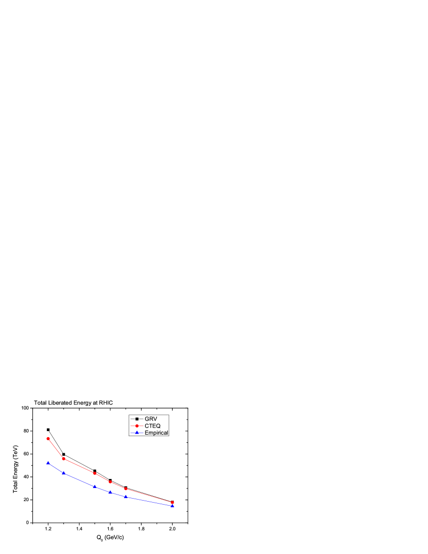
Figure 1: Total energy liberated from Au-Au at 200 GeV/pair.

Fig. 2 shows the total energy liberated at LHC which has 1140 TeV available CM energy. GRV simulation gives more energy deposition than the other two distributions. Assuming that the liberated energy into minijets is about 70-80%, we can estimate the minimum momentum transfer is 3.5-3.7 GeV/c for CTEQ distribution and 3.7-3.9 GeV/c for GRV model. These numbers are much larger than those of educated theoretical prediction, $Q_{0}^{2}=2-3GeV^{2}/c^{2}$.

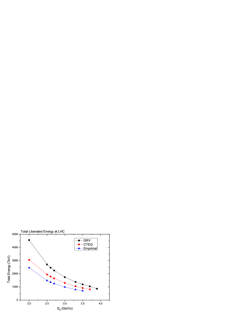
Figure 2: Total energy liberated from Pb-Pb at 5.5 TeV/pair.

Fig. 3 shows the total number of produced partons at RHIC as a function of $Q_{0}$ and the number of produced partons is about 3700 with CTEQ at $Q_{0}=1.7$ GeV/c, which liberates about 70% of total energy. Fig. 4 shows the total number of produced partons at LHC as function of $Q_{0}$. The total number of partons with CTEQ is about 11700 at $Q_{0}=3.5$ GeV/c which liberates about 80% of CM energy at LHC. CTEQ predicts more parton production than the others at RHIC but GRV gives far more partons at LHC, which means GRV distribution have more increasement than the others as $x$ gets smaller.

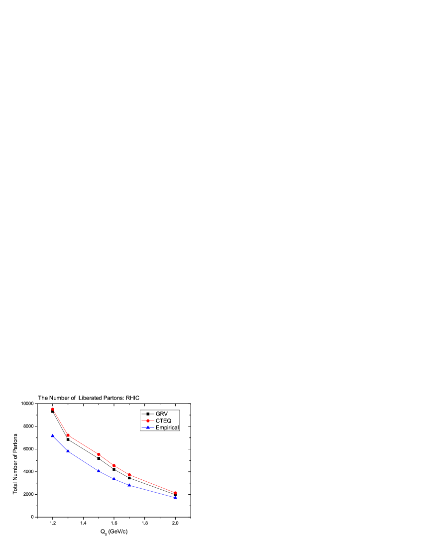
Figure 3: Total number of partons produced at RHIC energy.

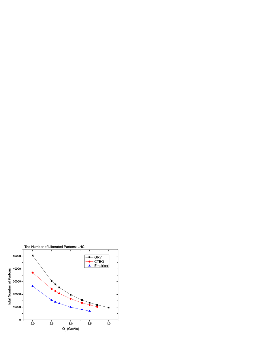
Figure 4: Total number of partons produced at LHC energy.

Table 1 gives the total numbers and the average energy in GeV of partons after a Au-Au collision at 200A GeV and a Pb-Pb collision at 5.5A TeV.

	RHIC: $Q_{0}$ = 1.7 GeV		LHC: $Q_{0}$ = 3.5 GeV
parton	N	$\bar{E}$	N	$\bar{E}$
g	3062	7.01	10380	66.8
u	230	13.9	356	235.7
d	255	14.5	384	253.3
s	33	7.9	122	79.9
$\bar{u}$	62	8.1	170	90.2
$\bar{d}$	61	8.2	168	92.0

Table 1: Initial distribution data: using CTEQ distribution function.

The table shows that most of partons produced at LHC energy are jets and the liberated valence quarks have extremely high energy. 30% of valence quarks are liberated from the colliding nuclei at RHIC and 32% at LHC so that substantial amount of baryons are provided into the parton system from the very beginning. We also note that the strangeness is produced from the primary collisions. These initial baryon and stageness contents should be imprinted in further evolution of the system.

Fig. 5 shows the number of gluons produced and energy distribution as a function of rapidity at RHIC energy.

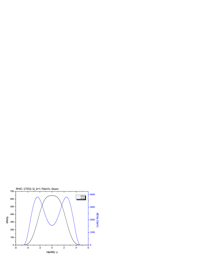
Figure 5: Gluon distribution as a function of rapidity at RHIC energy.

Even though the gluons are flat and high at central rapidity region, those gluons are strongly oriented in forward and backward direction energetically. We estimate the ${{dE}\over{dy}}/{{dN}\over{dy}}$ $\approx 2.3$ GeV at central rapidity region. This average energy of parton at central rapidity region is much lower than that of minijets. Fig. 6 shows the number of u-quarks produced and the energy distribution as a function of rapidity at RHIC energy. We can see clearly majority of partons move forward or backward in number and energy, which are mostly valence quarks.

Figure 6: u-quark distribution as a function of rapidity at RHIC.

On the other hand, fig. 7 shows the number of gluons produced and the energy distribution as a function of rapidity at LHC energy. The average energy per gluon is ${{dE}\over{dy}}/{{dN}\over{dy}}$ $\approx 5.7$ GeV at central rapidity region. This average energy is more than 10 times smaller compared to those of jets.

Figure 7: Gluon distribution as a function of rapidity at LHC energy.

Fig. 8 shows the number of u-quarks produced and the energy distribution as a function of rapidity at LHC energy.

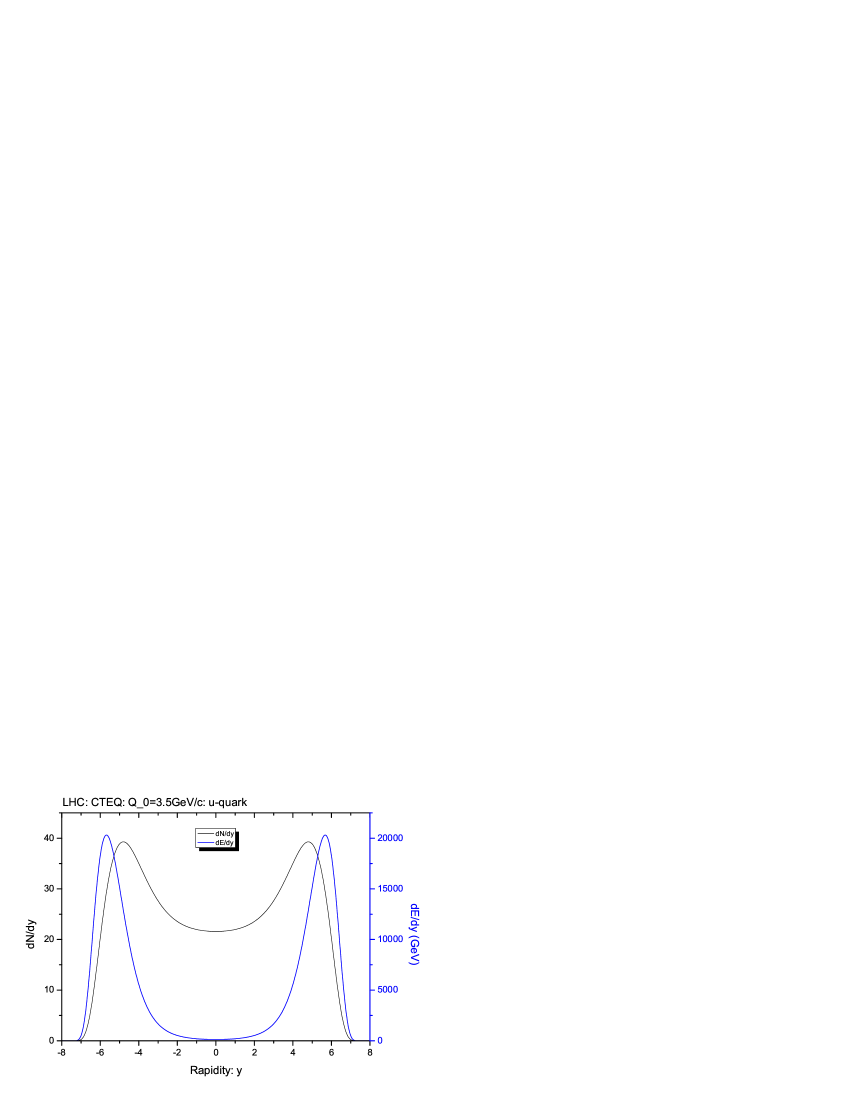
Figure 8: u-quark distribution as a function of rapidity at LHC.

Fig. 9 shows the number density $dN/dy$ at central rapidity region using the KNV function as a function of the saturation momentum, $Q_{s}$, where the saturation momentum $Q_{s}$ is different from the minimum momentum transfer $Q_{0}$. Assuming that the distribution is flat inbetween -2.5 and +2.5 and falls off to zero at $\pm 5$ linearly, the number of parton produced can be obtained by integration over transverse momentum and rapidity. This number however depends on the saturation momentum, $Q_{s}$, which is introduced in CGC scheme and estimated to be 1 GeV/c $<$ $Q_{s}$ $<$ 2 GeV/c at RHIC energy. The total number of initial partons is about 5400 for the $Q_{s}=1.7$ GeV/c and 4200 for the $Q_{s}=1.5$ GeV/c. We can see that the gluon density at central rapidity region at $Q_{0}=1.7$ GeV/c is compared to that of KNV results with $Q_{s}=1.7$ GeV/c at RHIC energy and that at $Q_{0}=3.5$ GeV/c compared to $Q_{s}=2.3$ GeV/c at LHC energy.

Figure 9: Number distribution of KNV distribution.

Fig. 10 and 11 show the rapidity distribution of quarks and antiquarks at RHIC and at LHC, respectively. We have more d-quarks than u-quarks since the Au or Pb have more neutrons than protons. The difference between a quark and its antiquark is the valence quark.

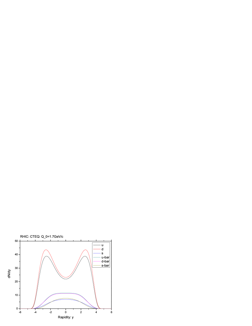
Figure 10: Number distribution of quarks and antiquarks.

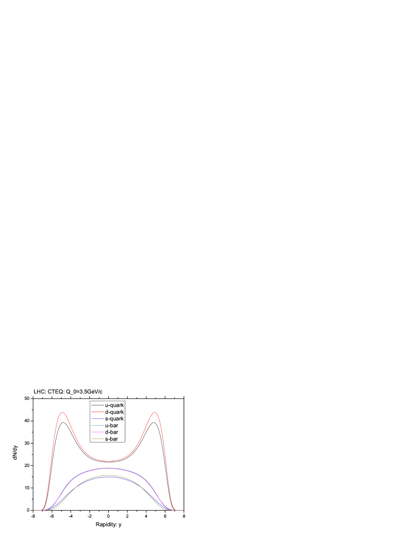
Figure 11: Rapidity distribution of quarks and antiquarks at LHC.

Fig. 12 and 13 give the energy and $p_{T}$ distributions of produced gluons and u-quarks at LHC.

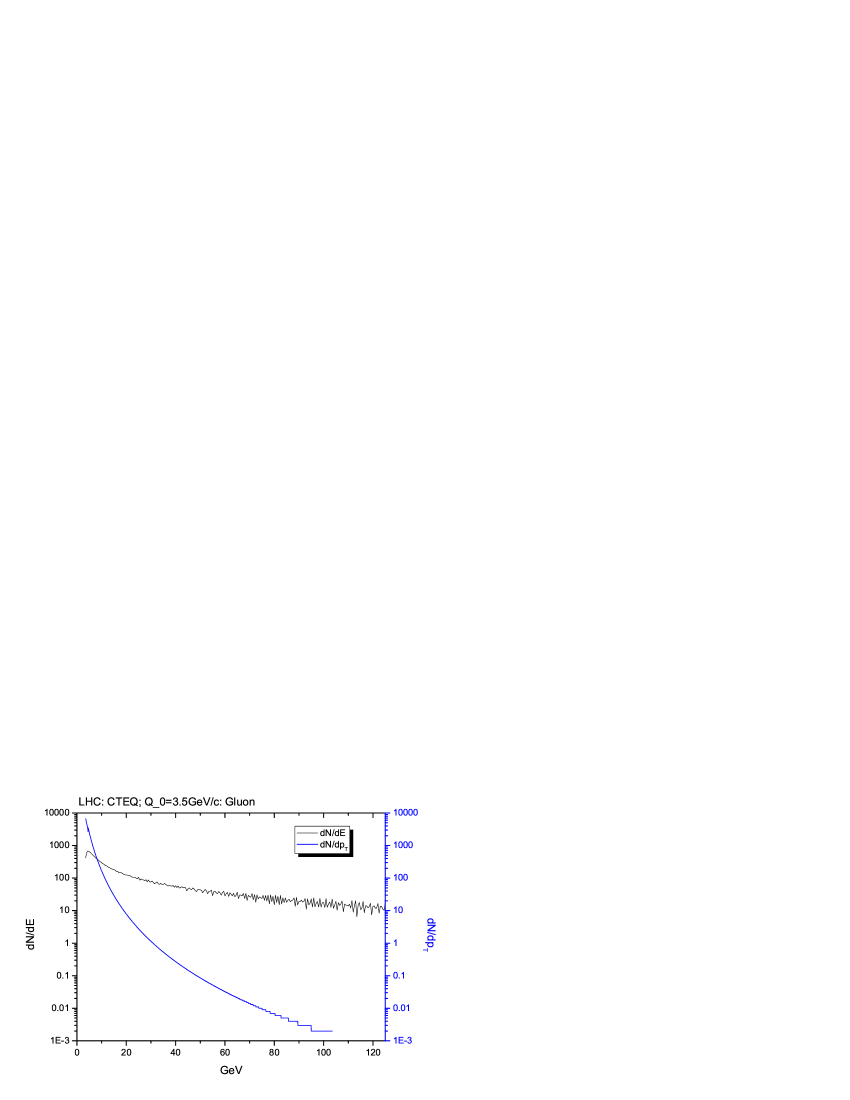
Figure 12: Energy and $p_{T}$ distribution of gluons at LHC.

Figure 13: Energy and $p_{T}$ distribution of quarks and antiquarks at LHC.

Fig. 14 and 15 give the energy and $p_{T}$ distributions of produced gluons and u-quarks at RHIC.

Figure 14: Energy and $p_{T}$ distribution of gluons at RHIC.

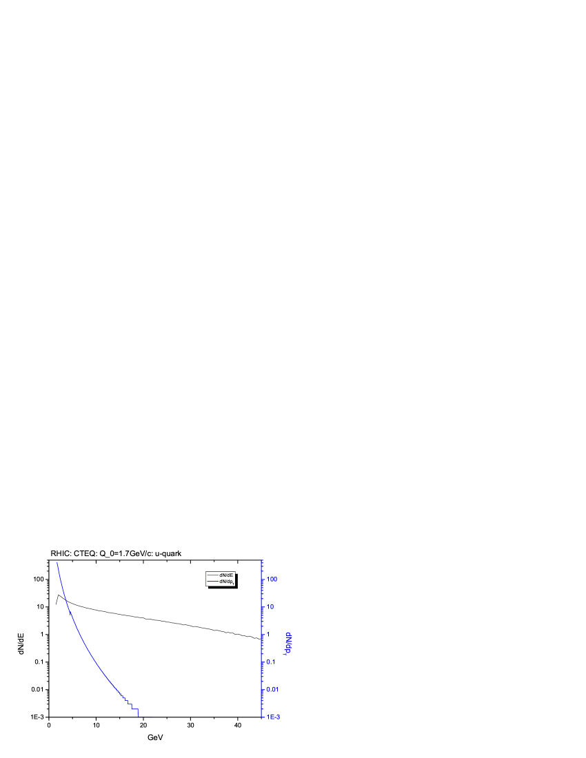
Figure 15: Energy and $p_{T}$ distribution of quarks and antiquarks at RHIC.

IV Summary and Conclusions

We showed total energy liberated from heavy ion collisions at RHIC and LHC energy and estimated the minimum momentum transfer, $Q_{0}$. We calculated the number of partons in detail produced from the collisions. We presented the rapidity distribution, energy distribution and $p_{T}$ distribution.

These distributions can be used as initial states to evolve the system. The partonic transport theory will be ideal to study the evolution of the system shin02 ; shin03 ; bla87 ; elze ; gyu97 ; gei92 as a function of time. We further note that these initial distributions could provide the initial condition for the hydrodynamic equation of motions.

Acknowledgement: This work was supported by the Korea Science and Engineering Foundation(KOSEF) under contract R01-2005-000-10334-0 and Kang Seog Lee is supported by the post-BK21 program.

References

- (1) Krasnitz A, Nara Y and Venugopalan R. Phys. Lett. B 554, 21 (2003); Nucl. Phys. A 717, 268 (2003).
- (2) Lappi T. Phys. Rev. C 67, 054903 (2003).
- (3) L. McLerran and R. Venugopalan, Phys. Rev. D49, 2233 (1994); 49, 3352 (1994); 50, 2225 (1994)
- (4) A. Mueller, Nucl. Phys. B572, 227 (2000).
- (5) D. Kharzeev, E. Levin and K. Tuchin, arXiv:hep-ph/0602063; D. Kharzeev and K. Tuchin, Nucl. Phys. A 753 (2005) 315 [arXiv:hep-ph/0501234].
- (6) STAR Collaboration, Nucl. Phys. A757, 102 (2005)
- (7) PHENIX Collaboration, Nucl. Phys. A757, 184 (2005)
- (8) J. Eskola, hep-ph/0210391.
- (9) G. C. Nayak, A. Dumitru, L. McLerran, and W. Greiner, Nucl. Phys. A687 457 (2001).
- (10) N. Hammon, H. Stocker, and W. Greiner, hep-ph/9903527.
- (11) F. Cooper, E. Mottola, and G. Nayak, hep-ph/0210391.
- (12) M. E. Peskin, D. V. Schroeder, Introduction to Quantum Field Theory, Addison-Wesley, 1995.
- (13) A. Szczuruk, arXiv:hep-ph/0304129.
- (14) G. R. Shin and B. Mueller, J. Phys. G 28, 2643 (2002).
- (15) G. R. Shin and B. Mueller, J. Phys. G 29, 2485 (2003); E. J. Chae, D. Y. Kim and Ghi R. Shin, JKPS 43, 473 (2003).
- (16) M. Glueck, E. Reya, and A. Vogt, hep-ph/9806404.
- (17) H. L. Lai, J. Huston, S. Kuhlmann, J. Morfin, F. Olness, J. F. Owens, J. Pumplin, W. K. Tung, Eur. Phys.J. C 12 (2000) 375; H. L. Lai, J. Huston, S. Kuhlmann, F. Olness, J. F. Owens, D. Soper, W. K. Tung, H. Weerts, Phys. Rev. D55 (1997) 1280.
- (18) J. Eskola, V.J. Kolhinen, and C.A. Salgado, Eur. Phys. J. C9 61 (1999), hep-ph/9807297; K. J. Eskola, V. J. Kolhinen, and P. V. Ruuskanen, Nucl. Phys. B535 351 (1998), hep-ph/9802350.
- (19) R. Baier, A. Kovner, U. Wiedemann, Phys. Rev. D68 (2003) 054009.
- (20) T. Hirano, Y. Nara, Nucl. Phys. A743 (2004) 305-328.
- (21) I. Arsene et al., Phys. Rev. Lett. 93 (2004) 102301; nucl-ex/0410020.
- (22) J. P. Blaizot and A. Mueller, Nucl. Phys. B289, 847 (1987).
- (23) B. Zhang, M. Gyulassy and Y. Pang, Phys.Rev. C58 (1998) 1175-1182
- (24) H.-Th. Elze and U. Heinz, Phys. Rep. 183 (1989) 81 and references therein.
- (25) K. Geiger and B. Müller, Nucl. Phys. B 369, 600 (1992); K. Geiger, Phys. Rev. D 46, 4965, and 4986 (1992); K. Geiger and J. I. Kapusta, Phys. Rev. D 47, 4905 (1993).