Long-range chiral dynamics of $\Lambda$-hyperon in nuclear media

Abstract

We extend a chiral effective field theory approach to the $\Lambda$-nuclei interaction with the inclusion of the decuplet baryons. More precisely, we study the contributions due to the long-range two-pion exchange, with $\Sigma$ and $\Sigma^{*}$ baryons in the internal baryonic lines considering Nh and $\Delta$h excitations. In particular, central and spin-orbit potentials are studied. For the former, regularization is needed and physical values of the cut-off give a large attraction, becoming necessary to include the repulsion of other terms not considered here. For the latter, in a model-independent framework, the inclusion of the decuplet supports the natural explanation of the smallness of the $\Lambda$-nuclear spin-orbit term and shows the importance of the $\Sigma^{*}$ and $\Delta$ degrees of freedom for the hyperon-nucleus interactions.

1 Introduction and framework

One of the most striking features of the $\Lambda$-nucleus potential is the weakness of the spin-orbit piece Bouyssy:1977jj ; Bruckner:1978ix . Several theoretical approaches have tried to explain it, ranging from one boson exchange (OBE) potentials Noble:1980kg with the couplings sometimes motivated by the underlying quark dynamics, to the consideration of two meson exchange pieces Brockmann:1977es or to quark based models Pirner:1979mb . Recently, a novel approach to the $\Lambda$-nucleus interaction based on effective field theory has attempted to explain this fact as a natural cancellation of short and long-range pieces Kaiser:2004fe . The main contribution to the $\Lambda$ mean field in that work comes from the first diagram in Fig.1, which is related to the nucleon-hole excitation contribution to the pion self-energy. However, we know from pion physics the importance of $\Delta$-hole excitation even at very low energy well below the $\Delta$ peak Oset:1981ih . Also, in Refs. Holzenkamp:1989tq ; Sasaki:2006cx it was shown the importance of the decuplet baryons as intermediate states in the two meson exchange terms of the $YN$ bare potential. The aim of this work is to extend the Ref. Kaiser:2004fe considering also the interaction with the relevant baryons of the decuplet ($\Delta$ and $\Sigma^{*}$) and its contribution to the two pion exchange potential. In particular, we will study whether the natural explanation of the weakness of the spin-orbit $\Lambda$-nucleus potential is still valid after the inclusion of the new terms. This paper reports briefly the results obtained in Camalich:2006is .

The coupling between the pseudoscalar meson octet and the baryon octet is given by

$${\cal L_{\rm oct}}=D\,{\rm Tr}\big{(}\bar{B}\gamma_{\mu}\gamma_{5}\{u^{\mu},B\}\big{)}+F\,{\rm Tr}\big{(}\bar{B}\gamma_{\mu}\gamma_{5}\big{[}u^{\mu},B\big{]}\big{)},$$ (1)

where $B$ is the traceless flavour matrix accounting for the spinors fields of baryons while $u^{\mu}=i[\xi^{\dagger},\partial^{\mu}\xi]/2$ introduce the SU(3) matrix of meson fields $\Phi$ since $\xi=Exp(i\Phi/\sqrt{2}f_{\pi})$. The interaction between the baryon octet, the baryon decuplet and the meson octet is described by Butler:1992pn :

Figure 1: Two pion exchange diagrams with $\Sigma$, $\Sigma^{*}$ in intermediate states and with 1Nh and 1$\Delta$h excitations of nuclear matter. Nucleon in-medium propagators are used.

$${\cal L_{\rm dec}}=\frac{{\cal C}}{\sqrt{2}f_{\pi}}\big{(}\bar{T_{\mu}}\partial^{\mu}\phi B+{\rm h.c.}\big{)},$$ (2)

where T${}^{\mu}_{abc}$ is the SU(3) representation for the 3/2⁺ spinor fields and where we have expanded the axial current up to one meson field. The parameter $f_{\pi}$=92.4 MeV is the weak pion decay constant and D=0.84, F=0.46 are the SU(3) axial-vector coupling constants for the octet baryons. The analysis of the partial decay widths of the decuplet shows a breaking of the SU(3) symmetry  Butler:1992pn ; Doring:2006ub of the order of 30%. In our calculation we need the $\Sigma^{*}\pi\Lambda$ and $\Delta\pi N$ vertices and we will use for each case as coupling constant ${\cal C}$ the value fitted to the decay widths of $\Sigma^{*}\rightarrow\pi\Lambda$ and $\Delta\rightarrow\pi N$ respectively (${\cal C}_{\Sigma*}=1.7,\,{\cal C}_{\Delta}=2.0$).

2 $\Lambda$-nucleus central potential depth

We focus on the obtainment of the density dependence of the mean-field $U_{\Lambda}(k_{f})$ for a zero-momentum $\Lambda$-hyperon interacting with an infinite isospin-symmetric nuclear matter via the long-range terms represented in Fig.1, (OPE interaction is prohibited by isospin conservation). The nucleon lines represent in medium nucleon propagators

$$G(p)=\frac{\theta(|\vec{p}|-k_{f})}{\gamma\cdot p-m+i\epsilon}+\frac{\theta(k_{f}-|\vec{p}|)}{\gamma\cdot p-m-i\epsilon}\,,$$ (3)

where $k_{f}$ is the Fermi momentum. We start with the first diagram of Fig.1 reproducing the procedure of Kaiser:2004fe . Two pieces, direct and crossed, appear in the pion self-energy after the N-hole loop energy integration. Moreover, each of them can be split into two other pieces, linear and quadratic in the occupation number $n(k)=\theta(k_{f}-|\vec{k}|)$.

A non-relativistic reduction is performed expanding the potentials in power series of a variable representative of the average mass of baryons, $M_{B}\equiv(2\,M_{N}+M_{\Lambda}+M_{\Sigma})/4$. Other relevant magnitudes are the mass splittings either on the internal-baryon line or on the 1ph excitation, expressed in a convenient way; $M_{\Sigma}-M_{\Lambda}\equiv\Delta^{2}/M_{B}\simeq 77$ MeV, $M_{\Sigma^{*}}-M_{\Lambda}\equiv{\Delta^{*}}^{2}/M_{B}\simeq 292$ MeV for the internal-line and $M_{\Delta}-M_{N}\equiv\Delta_{f}^{2}/M_{B}\simeq 270$ MeV for the 1ph.

Once integrated the energy in both loops, the direct term proportional to occupation number in the first diagram of Fig.1 gives to leading order the following contribution to the mean-field:

$${\small U_{\Lambda}(k_{f})^{\rm Nh-l}=-\frac{D^{2}g_{A}^{2}}{f_{\pi}^{4}}\int_{\mid\vec{p_{1}}\mid<k_{f}}\frac{d^{3}p_{1}d^{3}l}{(2\pi)^{6}}\times}$$

$${\small\times\frac{M_{B}\,\vec{l}^{4}}{(m_{\pi}^{2}+\vec{l}^{2})^{2}(\Delta^{2}+\vec{l}^{2}-\vec{l}\cdot\vec{p_{1}})},}$$ (4)

where $g_{A}=D+F=1.3$, $m_{\pi}$=138 MeV, $\vec{l}$ is the trimomentum of the pion and $\vec{p_{1}}$ is the trimomentum of the nucleon. The $d^{3}l$ loop is linearly ultraviolet divergent and we regularize it with a cut-off $\bar{\Lambda}=0.6$ GeV. The direct term, quadratic in occupation number in Fig.1 is a repulsive piece that, at leading order, gives

$${\small U_{\Lambda}(k_{f})^{\rm Nh-q}=\frac{D^{2}g_{A}^{2}}{f_{\pi}^{4}}\int_{\mid\vec{p}_{1,2}\mid<k_{f}}\frac{d^{3}p_{1}d^{3}p_{2}}{(2\pi)^{6}}\times}$$

$${\small\times\frac{M_{B}\,(\vec{p_{1}}-\vec{p_{2}})^{4}}{[m_{\pi}^{2}+(\vec{p_{1}}-\vec{p_{2}})^{2}]^{2}[\Delta^{2}+\vec{p_{2}}^{2}-\vec{p_{1}}\cdot\vec{p_{2}}]},}$$ (5)

where we have introduced a suitable change of variables $\vec{p_{1}}+\vec{l}=\vec{p_{2}}$. On the other hand, crossed terms are ignored since their leading order contributions are ${\cal O}$(1).

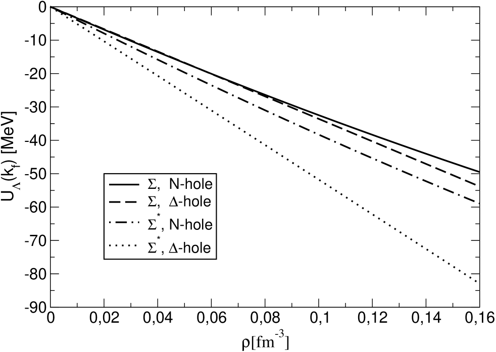
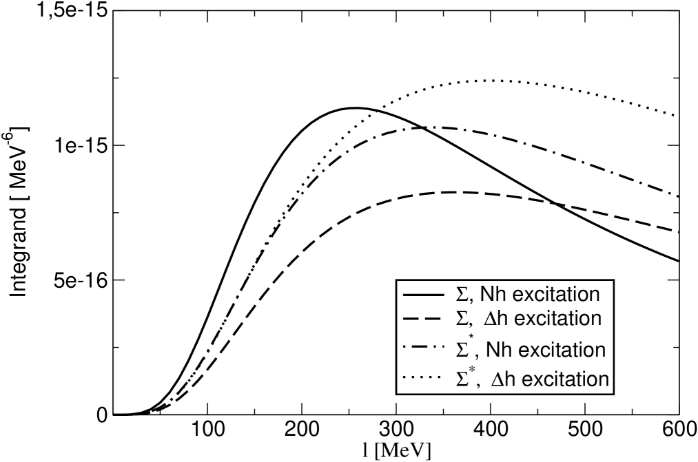
Figure 2: Left: Central potential dependence on nuclear medium density for diagrams presented in Fig.1. Right: Integrands of divergent pieces for a particular angular configuration ($\vec{l}\cdot\vec{p_{1}}=0$) and where a factor $\vec{l}^{2}$ has been omitted.

We compute now the second diagram of Fig.1, which considers a $\Delta$-h instead of a N-h excitation, integrating the loop energies and expanding to leading order in $M_{B}$. We find that its unique contribution is

$${\small U_{\Lambda}(k_{f})^{\rm\Delta h}=-\frac{8\,D^{2}{\cal C}_{\Delta}^{2}}{9\,f_{\pi}^{4}}\int_{\mid\vec{p_{1}}\mid<k_{f}}\frac{d^{3}p_{1}d^{3}l}{(2\pi)^{6}}\times}$$

$${\small\times\frac{M_{B}\,\vec{l}^{4}}{(m_{\pi}^{2}+\vec{l}^{2})^{2}(\Delta^{2}+\Delta_{f}^{2}+\vec{l}^{2}-\vec{l}\cdot\vec{p_{1}})}}.$$ (6)

The analytical structure of this piece is the same as in (4) but with a new splitting term in the denominator and a different coefficient. The integral diverges and the previous regulator $\bar{\Lambda}$ is used.

Third and fourth diagrams consider the hyperon $\Sigma^{*}(1385)$ instead of $\Sigma$ as intermediate state. A calculation using the procedure shown above leads to similar equations as (4), (5) and (6) but with different mass splittings in the denominator and different coefficients in front of them:

$${\small U^{*}_{\Lambda}(k_{f})^{\rm Nh-l}=-\frac{{\cal C}_{\Sigma*}^{2}g_{A}^{2}}{2\,f_{\pi}^{4}}\int_{\mid\vec{p_{1}}\mid<k_{f}}\frac{d^{3}p_{1}d^{3}l}{(2\pi)^{6}}\times}$$ (7)

$${\small\times\frac{M_{B}\,\vec{l}^{4}}{(m_{\pi}^{2}+\vec{l}^{2})^{2}({\Delta^{*}}^{2}+\vec{l}^{2}-\vec{l}\cdot\vec{p_{1}})},}$$ (8)

$${\small U^{*}_{\Lambda}(k_{f})^{\rm Nh-q}=\frac{{\cal C}_{\Sigma*}^{2}g_{A}^{2}}{2\,f_{\pi}^{4}}\int_{\mid\vec{p}_{1,2}\mid<k_{f}}\frac{d^{3}p_{1}d^{3}p_{2}}{(2\pi)^{6}}\times}$$

$${\small\times\frac{M_{B}\,(\vec{p_{1}}-\vec{p_{2}})^{4}}{[m_{\pi}^{2}+(\vec{p_{1}}-\vec{p_{2}})^{2}]^{2}[{\Delta^{*}}^{2}+\vec{p_{2}}^{2}-\vec{p_{1}}\cdot\vec{p_{2}}]},}$$ (9)

$${\small U^{*}_{\Lambda}(k_{f})^{\rm\Delta h}=-\frac{{4\,\cal C}_{\Sigma*}^{2}{\cal C}_{\Delta}^{2}}{9\,f_{\pi}^{4}}\int_{\mid\vec{p_{1}}\mid<k_{f}}\frac{d^{3}p_{1}d^{3}l}{(2\pi)^{6}}\times}$$

$${\small\times\frac{M_{B}\,\vec{l}^{4}}{(m_{\pi}^{2}+\vec{l}^{2})^{2}({\Delta^{*}}^{2}+\Delta_{f}^{2}+\vec{l}^{2}-\vec{l}\cdot\vec{p_{1}})}.}$$ (10)

Again, the integral of Eq. (9) is convergent, while the integration of (8), (10) are regularized with the momentum cut-off $\bar{\Lambda}$.

A simple estimation of the amplitudes being integrated can give a hint of the relative importance of the different contributions of Fig.1 to the low-momenta interaction. At first glance, decuplet-baryon diagrams are suppressed by heavier terms in the denominator, but they are also enhanced, on the other hand, by the stronger couplings introduced by the $MBB^{*}$ vertices. That would give, from $\frac{1}{\Delta^{2}+l^{2}}$ to $\frac{2.0}{\Delta^{2}+\Delta^{2}_{f}+l^{2}}$, $\frac{3.1}{{\Delta^{*}}^{2}+l^{2}}$ or $\frac{6.3}{{\Delta^{*}}^{2}+\Delta^{2}_{f}+l^{2}}$ for the comparison between the first diagram (Fig.1) and the second, the third or the fourth respectively. This comparison is illustrated also in Fig.2 (Right) where the integrands of the dominant pieces for a particular angular configuration are drawn along the interval of integration. All this shows how the extra damping in the new diagrams introduced by the larger mass splittings is compensated by the stronger couplings of the pion to the decuplet.

The density dependence of the different pieces of the potential is presented in Fig.2 (Left)). The value given by these diagrams at saturation density is strongly attractive

$$U^{\rm l-r}_{\Lambda}(\rho_{0})\simeq-250,{\rm MeV}$$ (11)

and consequently short-range terms have to be introduced in order to get a realistic central-potential depth. See, for instance, Ref. Tolos:2006ny where the inclusion of short range correlations in these pieces leads to reasonable total potentials.

3 $\Lambda$-nucleus spin-orbit potential

The spin-orbit coupling is described by the spin-dependent part of the self-energy produced when we consider the interaction of the corresponding particle (in our case a $\Lambda$-hyperon) with a weakly inhomogeneous medium. This is achieved Kaiser:2004fe considering that the $\Lambda$-hyperon scatters from an initial trimomentum $\vec{p}-\vec{q}/2$ to a final trimomentum $\vec{p}+\vec{q}/2$. Then, the dominant spin-dependent part for such weak inhomogeneity arises as

$$\Sigma_{\rm spin}=\frac{i}{2}\vec{\sigma}\cdot(\vec{q}\times\vec{p})U_{\Lambda ls}(k_{f0}).$$ (12)

The spin-orbit strength is identified with the shell-model spin-orbit potential when we multiply by a normalized density profile $f(r)$ and express the result in coordinate space by a Fourier transform:

$${\cal H}_{\Lambda ls}=U_{\Lambda ls}(k_{f0})\frac{1}{2r}\frac{df(r)}{dr}\,\vec{\sigma}\cdot{\vec{L}},$$ (13)

where $\vec{L}$ is the orbital angular momentum of the $\Lambda$-hyperon.

The antisymmetric vectorial structure of (12) can be obtained manipulating the expression $\vec{\sigma}\cdot(\vec{l}+\vec{q}/2)\vec{\sigma}\cdot(\vec{l}+\vec{q}/2)$ coming from the $\pi\Sigma\Lambda$ vertices in the two first diagrams of Fig.1, and also $\vec{S}\cdot(\vec{l}+\vec{q}/2)\vec{S}^{\dagger}\cdot(\vec{l}+\vec{q}/2)$ from the $\pi\Sigma^{*}\Lambda$ vertices of the two last diagrams of Fig.1. Using the known relations

$$\sigma_{i}\sigma_{j}=\delta_{ij}+i\epsilon_{ijk}\sigma_{k}$$ (14)

and

$$S_{i}S^{\dagger}_{j}=2/3\,\delta_{ij}-i/3\,\epsilon_{ijk}\sigma_{k}$$ (15)

we obtain the antisymmetric tensorial structure which characterizes the spin-dependent part of the self-energy of Eq. (12). Notice that these terms have a different sign depending on the SU(3)-multiplet which the internal-line baryon belongs to, circumstance that produces cancellations between the diagrams with $\Sigma$ and the diagrams with $\Sigma^{*}$. The other factor $\vec{p}$  is in the denominator and comes up after expanding the amplitude in a power series and keeping the linear term. Finally, we obtain the following $\Lambda$-nucleus spin-orbit potentials for the different diagrams:

$${\small U_{\Lambda ls}(k_{f})^{\rm Nh-l}=-\frac{2D^{2}g_{A}^{2}}{3f_{\pi}^{4}}\int_{\mid\vec{p_{1}}\mid<k_{f}}\frac{d^{3}p_{1}d^{3}l}{(2\pi)^{6}}\times}$$

$${\small\times\frac{M_{B}\,\vec{l}^{4}}{(m_{\pi}^{2}+\vec{l}^{2})^{2}(\Delta^{2}+\vec{l}^{2}-\vec{l}\cdot\vec{p_{1}})^{2}},}$$ (16)

$${\small U_{\Lambda ls}(k_{f})^{\rm Nh-q}=\frac{2D^{2}g_{A}^{2}}{3f_{\pi}^{4}}\int_{\mid\vec{p}_{1,2}\mid<k_{f}}\frac{d^{3}p_{1}d^{3}p_{2}}{(2\pi)^{6}}\times}$$

$${\small\times\frac{M_{B}\,(\vec{p_{1}}-\vec{p_{2}})^{4}}{[m_{\pi}^{2}+(\vec{p_{1}}-\vec{p_{2}})^{2}]^{2}[\Delta^{2}+\vec{p_{2}}^{2}-\vec{p_{1}}\cdot\vec{p_{2}}]^{2}},}$$ (17)

$${\small U_{\Lambda ls}(k_{f})^{\rm\Delta h}=-\frac{16\,D^{2}{\cal C}_{\Delta}^{2}}{27\,f_{\pi}^{4}}\int_{\mid\vec{p_{1}}\mid<k_{f}}\frac{d^{3}p_{1}d^{3}l}{(2\pi)^{6}}\times}$$

$${\small\times\frac{M_{B}\,\vec{l}^{4}}{(m_{\pi}^{2}+\vec{l}^{2})^{2}(\Delta^{2}+\Delta_{f}^{2}+\vec{l}^{2}-\vec{l}\cdot\vec{p_{1}})^{2}},}$$ (18)

$${\small U^{*}_{\Lambda ls}(k_{f})^{\rm Nh-l}=\frac{\,{\cal C}_{\Sigma*}^{2}g_{A}^{2}}{6\,f_{\pi}^{4}}\int_{\mid\vec{p_{1}}\mid<k_{f}}\frac{d^{3}p_{1}d^{3}l}{(2\pi)^{6}}\times}$$

$${\small\times\frac{M_{B}\,\vec{l}^{4}}{(m_{\pi}^{2}+\vec{l}^{2})^{2}({\Delta^{*}}^{2}+\vec{l}^{2}-\vec{l}\cdot\vec{p_{1}})^{2}},}$$ (19)

$${\small U^{*}_{\Lambda ls}(k_{f})^{\rm Nh-q}=-\frac{{\cal C}_{\Sigma*}^{2}g_{A}^{2}}{6\,f_{\pi}^{4}}\int_{\mid\vec{p}_{1,2}\mid<k_{f}}\frac{d^{3}p_{1}d^{3}p_{2}}{(2\pi)^{6}}\times}$$

$${\small\times\frac{M_{B}\,(\vec{p_{1}}-\vec{p_{2}})^{4}}{[m_{\pi}^{2}+(\vec{p_{1}}-\vec{p_{2}})^{2}]^{2}[{\Delta^{*}}^{2}+\vec{p_{2}}^{2}-\vec{p_{1}}\cdot\vec{p_{2}}]^{2}},}$$ (20)

$${\small U^{*}_{\Lambda ls}(k_{f})^{\rm\Delta h}=\frac{4\,{\cal C}_{\Sigma*}^{2}{\cal C}_{\Delta}^{2}}{27\,f_{\pi}^{4}}\int_{\mid\vec{p_{1}}\mid<k_{f}}\frac{d^{3}p_{1}d^{3}l}{(2\pi)^{6}}\times}$$

$${\small\times\frac{M_{B}\,\vec{l}^{4}}{(m_{\pi}^{2}+\vec{l}^{2})^{2}({\Delta^{*}}^{2}+\Delta_{f}^{2}+\vec{l}^{2}-\vec{l}\cdot\vec{p_{1}})^{2}}.}$$ (21)

All these integrations are convergent and therefore don’t depend in other input parameters than the coupling constants and particle masses. Notice also that these contributions account for non-relativistic effects since they arise at leading order in $M_{B}$ expansion. This is a different situation to that which emerges in mean-field models with OBE interactions, where the spin-orbit interaction is a relativistic effectBrockmann:1977es2 .We have checked numerically that the expansion in the $M_{B}$ is good, even when the mass splittings are almost 300 MeV. The difference at $\rho=\rho_{0}$ is less than 10% for all diagrams. In Fig. 3, it is shown the density dependence of the spin-orbit potentials calculated in this manner. The $\Delta$-hole diagram (second diagram of Fig.1) gives a contribution similar in size and of the same sign as the $N$-hole diagram (first). This would spoil the result of Kaiser:2004fe and produce a too large negative contribution. However, the processes with a $\Sigma^{*}$ have a positive contribution giving a total result quite similar to that obtained previously including only the first diagram. As explained before, this different sign comes from the opposite sign of the antisymmetric parts of Eqs. (14) and (15), which correspond to octet-octet and octet-decuplet spin transition operators respectively.

We also show in Fig. 3 a rough estimate of the total result by using the same approach as in Ref. Kaiser:2004fe to account for the missing short range pieces. A full discussion justifying this approach can be found there. We take

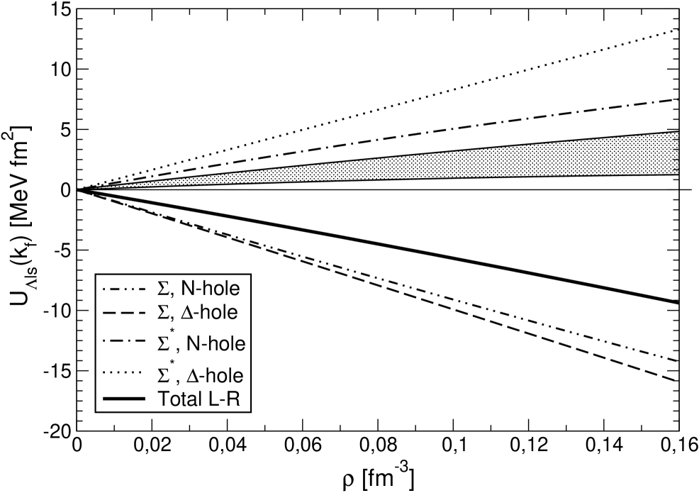
Figure 3: Spin-Orbit potential $U_{\Lambda ls}(k_{f})$ of a $\Lambda$-hyperon in isospin-symmetric nuclear matter for the Fig.1 diagrams and for the full model added to the short-range parametrization (shaded area). The short-range parametrization is $U_{\Lambda ls}^{\rm shell}(k_{f})$=21.3$C_{l}$ MeV fm² $\rho$/$\rho_{0}$ where $C_{l}$ lies between 1/2 and 2/3.

$$U_{\Lambda ls}^{\rm shell}(k_{f})=C_{l}\frac{M_{N}^{2}}{M_{\Lambda}^{2}}U_{Nls}^{\rm shell}(k_{f})$$ (22)

where the factor $M_{N}^{2}/M_{\Lambda}^{2}$ comes from the replacement of the nucleon by the $\Lambda$-hyperon in these relativistic spin-orbit terms. For $U_{Nls}^{\rm shell}(k_{f})$ we suppose a linear dependence in $\rho$ that takes the value 30 MeV fm³ at saturation density Chabanat:1997un . For $C_{l}$ we take the band between the values 1/2 and 2/3.

References

• (1) A. Bouyssy, Nucl. Phys. A 290 (1977) 324.
• (2) W. Bruckner et al. [Heidelberg-Saclay-Strasbourg Collaboration], Phys. Lett. B 79 (1978) 157; M. May et al., Phys. Rev. Lett.  47 (1981) 1106; M. May et al., Phys. Rev. Lett.  51 (1983) 2085; S. Ajimura et al., Phys. Rev. Lett.  86 (2001) 4255.
• (3) J. V. Noble, Phys. Lett. B 89 (1980) 325; C. B. Dover and A. Gal, Prog. Part. Nucl. Phys.  12 (1985) 171. B. K. Jennings, Phys. Lett. B 246 (1990) 325; E. Hiyama, M. Kamimura, T. Motoba, T. Yamada and Y. Yamamoto, Phys. Rev. Lett.  85 (2000) 270.
• (4) R. Brockmann and W. Weise, Phys. Lett. B 69 (1977) 167.
• (5) H. J. Pirner, Phys. Lett. B 85 (1979) 190; K. Tsushima, K. Saito, J. Haidenbauer and A. W. Thomas, Nucl. Phys. A 630, 691 (1998) [arXiv:nucl-th/9707022]; Y. Fujiwara, M. Kohno, T. Fujita, C. Nakamoto and Y. Suzuki, Nucl. Phys. A 674, 493 (2000) [arXiv:nucl-th/9912047].
• (6) N. Kaiser and W. Weise, Phys. Rev. C 71 (2005) 015203 [arXiv:nucl-th/0410062].
• (7) E. Oset, H. Toki and W. Weise, Phys. Rept.  83 (1982) 281.
• (8) B. Holzenkamp, K. Holinde and J. Speth, Nucl. Phys. A 500 (1989) 485.
• (9) K. Sasaki, E. Oset and M. J. Vicente Vacas, accepted in Phys. Rev. C, arXiv:nucl-th/0607068.
• (10) J. M. Camalich and M. J. V. Vacas, arXiv:nucl-th/0611082.
• (11) M. N. Butler, M. J. Savage and R. P. Springer, Nucl. Phys. B 399 (1993) 69 [arXiv:hep-ph/9211247].
• (12) M. Doring, E. Oset and S. Sarkar, accepted in Phys. Rev. C, arXiv:nucl-th/0601027.
• (13) L. Tolos, A. Ramos and E. Oset, Phys. Rev. C 74 (2006) 015203 [arXiv:nucl-th/0603033].
• (14) R. Brockmann and W. Weise, Phys. Rev. C 16 (1977) 1282.
• (15) E. Chabanat, P. Bonche, P. Haensel, J. Meyer and R. Schaeffer, Nucl. Phys. A 635 (1998) 231.