Four-nucleon scattering: ab initio calculations in momentum space

Abstract

The four-body equations of Alt, Grassberger and Sandhas are solved for $n\text{-}{}^{3}\mathrm{H}$ scattering at energies below three-body breakup threshold using various realistic interactions including one derived from chiral perturbation theory. After partial wave decomposition the equations are three-variable integral equations that are solved numerically without any approximations beyond the usual discretization of continuum variables on a finite momentum mesh. Large number of two-, three- and four-nucleon partial waves are considered until the convergence of the results is obtained. The total $n\text{-}{}^{3}\mathrm{H}$ cross section data in the resonance region is not described by the calculations which confirms previous findings by other groups. Nevertheless the numbers we get are slightly higher and closer to the data than previously found and depend on the choice of the two-nucleon potential. Correlations between the $A_{y}$ deficiency in $n\text{-}d$ elastic scattering and the total $n\text{-}{}^{3}\mathrm{H}$ cross section are studied.

I Introduction

The four-nucleon $(4N)$ scattering problem gives rise to the simplest set of nuclear reactions that shows the complexity of heavier systems. The neutron-${}^{3}\mathrm{H}$ $(n\text{-}{}^{3}\mathrm{H})$ and proton-${}^{3}\mathrm{He}$ $(p\text{-}{}^{3}\mathrm{He})$ scattering is dominated by the total isospin $\mathcal{T}=1$ states while deuteron-deuteron $(d\text{-}d)$ scattering by the $\mathcal{T}=0$ states; the reactions $n\text{-}{}^{3}\mathrm{He}$ and $p\text{-}{}^{3}\mathrm{H}$ involve both $\mathcal{T}=0$ and $\mathcal{T}=1$ and are coupled to $d\text{-}d$ in $\mathcal{T}=0$. Due to the charge dependence of the hadronic and electromagnetic interaction a small admixture of $\mathcal{T}=2$ states is also present. In $4N$ scattering the Coulomb interaction is paramount not only to treat $p\text{-}{}^{3}\mathrm{He}$ but also to separate the $n\text{-}{}^{3}\mathrm{He}$ threshold from $p\text{-}{}^{3}\mathrm{H}$ and at the same time avoid a second excited state of the $\alpha$ particle a few keV bellow the lowest scattering threshold. All these complex features make the $4N$ scattering problem not only a natural theoretical laboratory to test different force models of the nuclear interaction, but also the next step in the pursuit of very accurate ab initio calculations of the $N$-body scattering problem after the extensive work on the three-nucleon $(3N)$ system that has taken place in the past twenty years by several groups gloeckle:96a ; golak:05a ; kievsky:01a .

In Refs. fonseca:99a ; fonseca:02a all the reactions mentioned above were studied in the framework of Alt, Grassberger, and Sandhas (AGS) equations grassberger:67 using the rank one representation of realistic two-nucleon $(2N)$ force models together with a high rank representation of all $3N$ subsystem amplitudes; the Coulomb interaction was neglected. This led to one-variable integral equations whose predictive power was limited to the quality of the involved approximations. The calculations showed large discrepancies with data, namely nucleon analyzing power $A_{y}$ in $n\text{-}{}^{3}\mathrm{He}$ scattering, tensor observables in ${}^{2}\mathrm{H}(\vec{d},n){}^{3}\mathrm{He}$ and ${}^{2}\mathrm{H}(\vec{d},d)^{2}\mathrm{H}$ and the differential cross section for ${}^{2}\mathrm{H}(d,n){}^{3}\mathrm{He}$, but one surprising success in describing the total cross section $\sigma_{t}$ for $n\text{-}{}^{3}\mathrm{H}$ scattering in the resonance region where at neutron lab energy $E_{n}\simeq 3.5$ MeV $\sigma_{t}$ rises to about 2.45 b phillips:80 . Calculations by the Grenoble group cieselski:99 using coordinate-space solutions of the Faddeev-Yakubovsky equations yakubovsky:67 showed, on the contrary, that realistic interactions missed the total cross section peak by at least 0.2 b. Although these calculations carried out no approximation on the treatment of the $2N$ interaction, they were limited vis-á-vis LABEL:~fonseca:99a on the number of $3N$ and $4N$ partial waves.

Although the issue was recently clarified lazauskas:04a ; lazauskas:05a by comparing to an independent calculation by the Pisa group that uses the Kohn variational method, together with hyperspherical harmonics, further studies based on the AGS equations are needed to settle this important problem because some of the results by the Grenoble and Pisa groups may be still of limited accuracy given the number of included $2N$, $3N$, and $4N$ partial waves. Further investigations are also needed for the understanding of other $4N$ reactions such as $p\text{-}{}^{3}\mathrm{He}$, $n\text{-}{}^{3}\mathrm{He}$ and $d\text{-}d$ where large discrepancies with data were previously found. One fundamental issue underlying four-nucleon physics is the existence of correlations between $3N$ and $4N$ observables. One of the best known is the Tjon line tjon:75 which correlates the binding energies of ${}^{3}\mathrm{H}$ with ${}^{4}\mathrm{He}$; another one involves the triton binding energy and the singlet (triplet) $n\text{-}{}^{3}\mathrm{H}$ scattering length viviani:98a . Nevertheless, other correlations may exist: one could ask if the persistent $A_{y}$ problem in $n\text{-}d$ scattering is in any way related to the failure to reproduce $\sigma_{t}$ in $n\text{-}{}^{3}\mathrm{H}$ scattering in the resonance region, or to the $A_{y}$ problem in $p\text{-}{}^{3}\mathrm{He}$ viviani:01a ; does resolving the former also solves the latter?

Therefore we present here a new numerical approach to the solution of the AGS equations that is both numerically exact and extremely fast in terms of CPU-time demand. Since the $2N$ transition matrix (t-matrix) is treated exactly, the equations we solve are, after partial wave decomposition, three-variable integral equations. The three Jacobi momentum variables in $1+3$ and $2+2$ configurations are discretized on a finite mesh and the number of $2N$, $3N$ and $4N$ partial waves increased up to what is needed for the full convergence of the observables. The present approach also allows for the inclusion of charge-dependent interactions as well as $\Delta$ degrees of freedom that lead to an effective $3N$ force. Furthermore, using the method recently proposed to treat the Coulomb force in $p\text{-}d$ elastic scattering and breakup deltuva:05a ; deltuva:05c ; deltuva:05d , we have already obtained preliminary results for $p\text{-}{}^{3}\mathrm{He}$ elastic scattering observables fonseca:fb18 with the Coulomb potential between the three protons included.

In Sec. II we discuss the integral equations we solve for $n\text{-}{}^{3}\mathrm{H}$ scattering and in Sec. III we show the results of our most complete calculations, leaving tests of benchmark to the Appendix. Finally conclusions come in Sec. IV.

II Equations

As initially proposed by Alt, Grassberger and Sandhas grassberger:67 and later reviewed for the purpose of practical applications in LABEL:~fonseca:87 , the four-particle scattering equations may be written in a matrix form

$$\mathcal{U}={} \mathcal{V}+\mathcal{V}\,\mathcal{G}_{0}\,\mathcal{U},$$ (1a)

$$\mathcal{U}|\Phi_{\rho_{0}}\rangle={} \mathcal{V}|\Psi_{\rho_{0}}\rangle,$$ (1b)

$$|\Psi_{\rho_{0}}\rangle={} |\Phi_{\rho_{0}}\rangle+\mathcal{G}_{0}\,\mathcal{V}|\Psi_{\rho_{0}}\rangle,$$ (1c)

where $|\Phi_{\rho_{0}}\rangle$ is the initial channel state, $|\Psi_{\rho_{0}}\rangle$ the full scattering state, and $\rho_{0}$ defines the two-body entrance channel. Both of them have 18 components, and the transition operator $\mathcal{U}$ as well as $\mathcal{V}$ and $\mathcal{G}_{0}$ are $18\times 18$ matrix operators with components

$$[\mathcal{V}]^{\sigma\rho}_{ij}={} (G_{0}\,t_{i}\,G_{0})^{-1}\,\bar{\delta}_{\sigma\rho}\,\delta_{ij},$$ (2a)

$$[\mathcal{G}_{0}]^{\sigma\rho}_{ij}={} G_{0}\,t_{i}\,G_{0}\,U^{\sigma}_{ij}G_{0}\,t_{j}\,G_{0}\,\delta_{\sigma\rho}.$$ (2b)

As usual, $\sigma(\rho)$ denotes two-cluster partitions of $1+3$ or $2+2$ type and $i(j)$ the pair interactions. $G_{0}$ is the four free particle Green’s function, $t_{i}$ is the two-particle t-matrix embedded in four-particle space, $\bar{\delta}_{\sigma\rho}=1-\delta_{\sigma\rho}$, and $U^{\sigma}_{ij}$ are the subsystem transition operators

$$U^{\sigma}_{ij}=G^{-1}_{0}\,\bar{\delta}_{ij}+\sum_{k}\bar{\delta}_{ki}\,t_{k}\,G_{0}\,U^{\sigma}_{kj}$$ (3)

of $1+3$ or $2+2$ type, depending on $\sigma$. If $\sigma$ is a $1+3$ partition, $U^{\sigma}_{ij}$ corresponds to the usual AGS transition matrix for the three interacting particles that are internal to $\sigma$. For $\sigma$ of $2+2$ type $U^{\sigma}_{ij}$ does not correspond to any physical process. The components of the initial/final two-cluster states $[|\Phi_{\rho_{0}}\rangle]^{\rho}_{i}=|\phi^{\rho_{0}}_{i}\rangle\delta_{\rho\rho_{0}}$ are the Faddeev components of the cluster bound state wave function times a plane wave of momentum ${\mathbf{p}}_{\rho_{0}}$ between clusters whose dependence is suppressed in our notation,

$$|\phi^{\rho_{0}}_{i}\rangle=G_{0}\,t_{i}\sum_{k}\bar{\delta}_{ki}|\phi^{\rho_{0}}_{k}\rangle.$$ (4)

The great advantage of AGS equations over the Yakubovsky equations is that on-shell matrix elements of $\mathcal{U}$ between initial $|\Phi_{\rho_{0}}\rangle$ and final $|\Phi_{\sigma_{0}}\rangle$ states with relative two-cluster momenta ${\mathbf{p}}_{\rho_{0}}$ and ${\mathbf{p}}^{\prime}_{\sigma_{0}}$ lead automatically to the corresponding scattering amplitudes

$$\langle{\mathbf{p}}^{\prime}_{\sigma_{0}}|T^{\sigma_{0}\rho_{0}}|{\mathbf{p}}_{\rho_{0}}\rangle={} \langle\Phi_{\sigma_{0}}|\mathcal{U}|\Phi_{\rho_{0}}\rangle$$ (5a)

$$={} \sum_{ij}\langle\phi^{\sigma_{0}}_{j}|\mathcal{U}^{\sigma_{0}\rho_{0}}_{ji}|\phi^{\rho_{0}}_{i}\rangle.$$ (5b)

For four identical particles the AGS equations reduce to $2\times 2$ matrix equations since there are only two distinct partitions, one of $1+3$ type and one of $2+2$ type, which we choose to be (12,3)4 and (12)(34); in the following we denote them by $\alpha=1$ and $\alpha=2$, respectively. In this case the equations may be conveniently written using the permutation operators $P_{ab}$ of particles $a$ and $b$ as it was done first in Refs. kamada:92a ; gloeckle:93a for the four-nucleon bound state. After the symmetrization of the four-nucleon scattering equations (1) we obtain equations of the same form but with new definitions for the symmetrized operators

$$\mathcal{V}^{\alpha\beta}={} (G_{0}\,t\,G_{0})^{-1}\,(\bar{\delta}_{\alpha\beta}-\delta_{\beta 1}P_{34}),$$ (6a)

$$\mathcal{G}_{0}^{\alpha\beta}={} G_{0}\,t\,G_{0}\,U^{\alpha}G_{0}\,t\,G_{0}\,\delta_{\alpha\beta}.$$ (6b)

Here $t$ is the pair (12) t-matrix, $U^{\alpha}$ the symmetrized 1+3 or 2+2 subsystem transition operators

$$U^{\alpha}=P_{\alpha}G_{0}^{-1}+P_{\alpha}t\,G_{0}\,U^{\alpha},$$ (7)

and $P_{\alpha}$ the permutation operators given by

$$P_{1}={} P=P_{12}\,P_{23}+P_{13}\,P_{23},$$ (8a)

$$P_{2}={} \tilde{P}=P_{13}\,P_{24}.$$ (8b)

The basis states are antisymmetric under exchange of two particles in subsystem (12) for $1+3$ partition and in (12) and (34) for $2+2$ partition. The symmetrized initial/final two-cluster state components are

$$|\phi^{\beta}\rangle=G_{0}\,tP_{\beta}|\phi^{\beta}\rangle.$$ (9)

The scattering amplitudes are obtained as

$$\langle{\mathbf{p}}^{\prime}_{\alpha}|T^{\alpha\beta}|{\mathbf{p}}_{\beta}\rangle=S_{\alpha\beta}\langle\phi^{\alpha}|\mathcal{U}^{\alpha\beta}|\phi^{\beta}\rangle,$$ (10)

where $S_{\alpha\beta}$ is a symmetrization factor; $S_{\alpha\alpha}=S_{\alpha}$ is the number of pairs internal to the partition $\alpha$, i.e., $S_{1}=3$ and $S_{2}=2$, and $S_{12}=2S_{21}=2\sqrt{3}$.

Since the present paper is confined to $n\text{-}{}^{3}\mathrm{H}$ scattering, we write down explicitly only the equations for the $1+3\to 1+3$ and $1+3\to 2+2$ transition operators

$$\mathcal{U}^{11}={} -(G_{0}\,t\,G_{0})^{-1}P_{34}-P_{34}U^{1}G_{0}\,t\,G_{0}\,\mathcal{U}^{11}$$

$$+U^{2}G_{0}\,t\,G_{0}\,\mathcal{U}^{21},$$ (11a)

$$\mathcal{U}^{21}={} (G_{0}\,t\,G_{0})^{-1}(1-P_{34})+(1-P_{34})U^{1}G_{0}\,t\,G_{0}\,\mathcal{U}^{11}.$$ (11b)

The equations coupling $\mathcal{U}^{12}$ and $\mathcal{U}^{22}$ share an identical kernel but different inhomogeneous terms.

After the partial wave expansion Eqs. (11) form a set of coupled integral equations with three variables corresponding to the Jacobi momenta $k_{x},\,k_{y}$ and $k_{z}$; the associated orbital angular momenta are denoted by $l_{x}$, $l_{y}$, and $l_{z}$, respectively. They are depicted in Fig. 1 for $1+3$ and $2+2$ configurations together with the pair total angular momentum $I$ and the the three-particle subsystem total angular momentum $J$. The states of total angular momentum $\mathcal{J}$ are defined as $|k_{x}\,k_{y}\,k_{z}[l_{z}(\{l_{y}[(l_{x}S_{x})I\,s_{y}]S_{y}\}Js_{z})S_{z}]\,\mathcal{JM}\rangle$ for the $1+3$ configuration and $|k_{x}\,k_{y}\,k_{z}(l_{z}\{(l_{x}S_{x})I\,[l_{y}(s_{y}s_{z})S_{y}]I^{\prime}\}S_{z})\mathcal{JM}\rangle$ for the $2+2$, where $s_{y}$ and $s_{z}$ are the spins of nucleons 3 and 4, and $S_{x}$, $S_{y}$, and $S_{z}$ are channel spins of two-, three-, and four-particle system. In all calculations $I$ and $I^{\prime}$ run over the same set of quantum numbers.

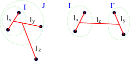
Figure 1: (Color online) Angular momentum quantum numbers for $1+3$ and $2+2$ basis states.

By the discretization of the momentum variables the integral equations may be turned into a system of linear equations but the direct solution is not possible because of the huge dimension. Therefore, in close analogy with three-nucleon scattering, we calculate the Neumann series for the on-shell matrix elements of the transition operators (11) and sum by the Padé method baker:75a . The Padé summation algorithm we use is described in LABEL:~chmielewski:03a . We work with the half-shell transition operators in the form

$$|X_{\alpha\beta}\rangle=G_{0}\,\mathcal{U}^{\alpha\beta}|\phi^{\beta}\rangle$$ (12)

such that the on-shell elements are $\langle\phi^{\alpha}|\mathcal{U}^{\alpha\beta}|\phi^{\beta}\rangle=\langle\xi_{\alpha}|X_{\alpha\beta}\rangle$ with the auxiliary states $|\xi_{\alpha}\rangle=G_{0}^{-1}|\phi^{\alpha}\rangle=tP_{\alpha}|\phi^{\alpha}\rangle$. Defining $Q_{\alpha}=G_{0}\,U^{\alpha}G_{0}\,t$ and using Eq. (9) for the inhomogeneous terms in order to eliminate $(G_{0}\,t\,G_{0})^{-1}$, Eqs. (11) become

$$|X_{11}\rangle={} -P_{34}P_{1}G_{0}|\xi_{1}\rangle-P_{34}Q_{1}|X_{11}\rangle+Q_{2}|X_{21}\rangle,$$ (13a)

$$|X_{21}\rangle={} (1-P_{34})P_{1}G_{0}|\xi_{1}\rangle+(1-P_{34})Q_{1}|X_{11}\rangle.$$ (13b)

In practical calculations, in order to accelerate the convergence of the Padé summation, it is advantageous to substitute Eq. (13b) into Eq. (13a) yielding the Neumann series

$$|X_{\alpha\beta}\rangle={} \sum_{n=0}^{\infty}|X_{\alpha\beta}^{(n)}\rangle,$$ (14a)

$$|X_{21}^{(0)}\rangle={} (1-P_{34})P_{1}G_{0}|\xi_{1}\rangle,$$ (14b)

$$|X_{11}^{(0)}\rangle={} -P_{34}P_{1}G_{0}|\xi_{1}\rangle+Q_{2}|X_{21}^{(0)}\rangle,$$ (14c)

$$|X_{21}^{(n)}\rangle={} (1-P_{34})Q_{1}|X_{11}^{(n-1)}\rangle,$$ (14d)

$$|X_{11}^{(n)}\rangle={} -P_{34}Q_{1}|X_{11}^{(n-1)}\rangle+Q_{2}|X_{21}^{(n)}\rangle,$$ (14e)

which requires $1+3$ and $2+2$ subsystem transition operators $U^{\alpha}$, contained in $Q_{\alpha}$, fully off-shell at different energies. Explicit calculation of $U^{\alpha}$ is not only very time consuming but also requires large storage devices. Therefore, except at the bound state poles, we do not calculate the full off-shell transition matrices $U^{\alpha}$ explicitly. Instead, we rewrite Eq. (7) as a Neumann series

$$U^{\alpha}=\sum_{r=0}^{\infty}(P_{\alpha}t\,G_{0})^{r}\,P_{\alpha}G_{0}^{-1}$$ (15)

resulting a corresponding Neumann series for the solution vectors in Eqs. (14), i.e.,

$$Q_{\alpha}|X_{\alpha\beta}^{(n)}\rangle={} \sum_{r=1}^{\infty}|X_{\alpha\beta}^{(n,r)}\rangle,$$ (16a)

$$|X_{\alpha\beta}^{(n,0)}\rangle={} |X_{\alpha\beta}^{(n)}\rangle,$$ (16b)

$$|X_{\alpha\beta}^{(n,r)}\rangle={} P_{\alpha}G_{0}\,t\,|X_{\alpha\beta}^{(n,r-1)}\rangle,$$ (16c)

where the summation again has to be performed using the Padé method. Usually, 6 to 18 Padé iteration steps are required for the convergence in Eqs. (14) - (16). At the bound state poles the subsystem transition operators are

$$U^{\alpha}=P_{\alpha}|\xi_{\alpha}\rangle\frac{S_{\alpha}}{E+i0-h_{0}^{z}-E_{B}}\langle\xi_{\alpha}|P_{\alpha},$$ (17)

where $E$ is the available four-nucleon energy, $E_{B}$ the binding energy, and $h_{0}^{z}$ the kinetic energy operator for the relative motion of the two clusters.

Thus, compared to the calculation of full off-shell $U^{\alpha}$, the method we are using avoids storage problems and also significantly reduces the number of required floating point operations, since it is essentially a calculation of half-shell matrix elements for a number of driving terms that are considerably fewer than the linear dimension of the discretized $U^{\alpha}$. A further advantage is that the matrices corresponding to the operators $P_{\alpha}$, $G_{0}$ and $t$ in Eq. (16c) have block-diagonal structure whereas $U^{\alpha}$ is a full matrix.

The calculation of the Neumann series (16) for $\alpha=1$ is what we are doing in three-nucleon scattering and is described in great detail in Refs. deltuva:03a ; deltuva:phd . The specific representation of the permutation operator $P_{1}$ where the initial and final state momenta $k_{y}$ are chosen as independent variables requires the interpolation in the momentum $k_{x}$ for the quantities on both sides of $P_{1}G_{0}$, i.e., for $t$ or $\langle\xi_{\alpha}|$. Two interpolation methods using Chebyshev polynomials and spline functions were used in LABEL:~deltuva:phd ; in the context of four-nucleon equations where one has to work with $1+3$ and $2+2$ basis states the spline interpolation is more convenient.

The calculation of the Neumann series (16) for $\alpha=2$ is straightforward because of the very simple form of the permutation operator $P_{2}$.

Finally, the application of the permutation operator $P_{34}$ as well as the transformation of $|X_{\alpha\beta}^{(n)}\rangle$ from $1+3$ basis to $2+2$ or vice versa has a structure similar to that of $P_{1}$, resulting in a similar treatment. The specific representation of $P_{34}$, i.e.,

$$\begin{split}\langle k_{x}k_{y}k_{z}|P_{34}|k^{\prime}_{x}k^{\prime}_{y}k^{\prime}_{z}\rangle={}&\frac{\delta(k_{x}-k^{\prime}_{x})}{k_{x}^{2}}\int_{-1}^{1}dy\;P_{34}(k_{z},k^{\prime}_{z},y)\\ &\times\frac{\delta(k_{y}-\bar{k}_{y}(k_{z},k^{\prime}_{z},y))}{k_{y}^{2}}\\ &\times\frac{\delta(k^{\prime}_{y}-\bar{k}^{\prime}_{y}(k_{z},k^{\prime}_{z},y))}{{k^{\prime}_{y}}^{2}},\end{split}$$ (18)

where the initial and final state momenta $k_{z}$ are chosen as independent variables, requires the interpolation in the momentum $k_{y}$ for the quantities on both sides of $P_{34}$ that are calculated on the mesh $\{k_{i_{y}}\}$. The dependence on the discrete quantum numbers is suppressed since it is irrelevant for the consideration as well as the explicit form of function $P_{34}(k_{z},k^{\prime}_{z},y)$. $\bar{k}^{\prime}_{y}(k_{z},k^{\prime}_{z},y)$ and and $\bar{k}_{y}(k_{z},k^{\prime}_{z},y)$ are the initial and final state Jacobi momenta $k_{y}$ expressed via $k^{\prime}_{z}$, $k_{z}$, and the angle between them $y=\hat{{\mathbf{k}}}^{\prime}_{z}\cdot\hat{{\mathbf{k}}}_{z}$. We use the spline interpolation again with the spline functions $S_{i_{y}}(k)$ boor:78a ; gloeckle:82a ; press:89a such that for the function $f(k)$, given on the mesh $\{k_{i_{y}}\}$, the values at any $k$ may be obtained by

$$f(k)\approx\sum_{i_{y}}f(k_{i_{y}})S_{i_{y}}(k).$$ (19)

For $P_{34}$ acting on the vector $|Y\rangle$ we obtain the following result (as a distribution)

$$\begin{split}\langle k_{x}k_{y}k_{z}|P_{34}|Y\rangle={}&\sum_{i_{y}}\frac{\delta(k_{y}-k_{i_{y}})}{k_{y}^{2}}\int_{0}^{\infty}{k^{\prime}_{z}}^{2}dk^{\prime}_{z}\int_{-1}^{1}dy\\ &\times S_{i_{y}}(\bar{k}_{y}(k_{z},k^{\prime}_{z},y))\,P_{34}(k_{z},k^{\prime}_{z},y)\\ &\times\sum_{j_{y}}S_{j_{y}}(\bar{k}^{\prime}_{y}(k_{z},k^{\prime}_{z},y))\,\langle k_{x}k_{j_{y}}k^{\prime}_{z}|Y\rangle\\ ={}&\sum_{i_{y}}\frac{\delta(k_{y}-k_{i_{y}})}{k_{y}^{2}}\tilde{Y}_{i_{y}}(k_{x},k_{z}),\end{split}$$ (20)

such that in the next step of the calculation, where the $\langle k_{x}k_{y}k_{z}|P_{34}|Y\rangle$ has to be multiplied by a smooth function $f(k_{y})$ and integrated over $k_{y}$, the result simply is the sum over the meshpoints $\{k_{i_{y}}\}$ for the involved quantities,

$$\int_{0}^{\infty}k_{y}^{2}dk_{y}\,f(k_{y})\langle k_{x}k_{y}k_{z}|P_{34}|Y\rangle=\sum_{i_{y}}f(k_{i_{y}})\,\tilde{Y}_{i_{y}}(k_{x},k_{z}).$$ (21)

The integrations in Eq. (20) are performed using Gaussian integration rules press:89a . The bound state pole (17) is treated by the subtraction technique much like the deuteron pole in the $n\text{-}d$ scattering deltuva:phd . Note that the representation of the operators $P_{1}$ and $P_{34}$ is different from the one used in Refs. kamada:92a ; nogga:02a where final state momenta $k_{y}$ and $k_{z}$ were chosen as independent variables.

III Results

In order to calibrate our work we start by reproducing results of previous calculations, in particular the binding energy of ${}^{4}\rm{He}$ obtained with different realistic $2N$ interactions by different groups nogga:02a ; kamada:01a ; lazauskas:04a ; viviani:06a as well as the $n\text{-}{}^{3}\mathrm{H}$ phase shifts obtained with Mafliet-Tjon potential by the Grenoble group lazauskas:phd . Furthermore, we check the numerical stability of our calculations. These results are presented in the Appendix and show that the present algorithm is numerically highly reliable and capable of reproducing previous published results.

Next we study the convergence of our calculations in terms of number of $2N$, $3N$, and $4N$ partial waves using the AV18 potential wiringa:95a for the $2N$ interaction. In the calculations presented here for the $n\text{-}{}^{3}\mathrm{H}$ scattering we include only the total isospin $\mathcal{T}=1$ states, but, within $\mathcal{T}=1$, we take into account all couplings resulting from the charge dependence of the interaction. Including $\mathcal{T}=2$ states would yield an effect that is of 2nd order in the charge dependence and, therefore, is expected to be extremely small much like the effect of the total $3N$ isospin $T=\frac{3}{2}$ states in elastic $n\text{-}d$ scattering. Coupling to $\mathcal{T}=2$ states is neglected also in all previous calculations, but in configuration-space treatments the isospin averaging within $\mathcal{T}=1$ states is performed for the potential, whereas we perform it for the t-matrix.

	$0^{+}\;(^{1}S_{0})$	$0^{-}\;(^{3}P_{0})$	$1^{+}\;(^{3}S_{1})$	$1^{-}\;(^{3}P_{1})$	$1^{-}\;(^{1}P_{1})$	$1^{-}\;(\epsilon)$	$2^{-}\;(^{3}P_{2})$	$\sigma_{t}$
$I\leq 1^{+}$	-69.54	20.97	-62.31	46.47	26.46	-37.74	36.19	2.106
$I\leq 1+{}^{3}P_{2}$	-70.60	22.82	-62.70	40.30	21.25	-44.00	43.53	2.151
$I\leq 2+{}^{3}D_{3}$	-70.02	24.43	-62.05	43.62	22.65	-44.46	47.06	2.301
$I\leq 3+{}^{3}F_{4}$	-69.68	23.52	-61.74	43.37	22.35	-44.71	46.71	2.277
$I\leq 4+{}^{3}G_{5}$	-69.63	23.62	-61.69	43.54	22.38	-44.69	47.03	2.288
$I\leq 5+{}^{3}H_{6}$	-69.61	23.56	-61.68	43.53	22.37	-44.73	47.00	2.286

Table 1: $n\text{-}{}^{3}\mathrm{H}$ phase shifts, $1^{-}$ mixing parameter $\epsilon$ (in degrees) and the total cross section $\sigma_{t}$ (in barns) at $E_{n}=4$ MeV neutron lab energy for increasing number of $2N$ partial waves and fixed $l_{y},l_{z}\leq 4$, $J\leq\frac{9}{2}$. The $2N$ potential is AV18.

	$0^{+}\;(^{1}S_{0})$	$0^{-}\;(^{3}P_{0})$	$1^{+}\;(^{3}S_{1})$	$1^{-}\;(^{3}P_{1})$	$1^{-}\;(^{1}P_{1})$	$1^{-}\;(\epsilon)$	$2^{-}\;(^{3}P_{2})$	$\sigma_{t}$
$l_{y},l_{z}\leq 0$	-69.70		-63.50					0.950
$l_{y},l_{z}\leq 1$	-69.59	22.62	-61.94	41.33	22.65	-44.49	43.35	2.163
$l_{y},l_{z}\leq 2$	-69.67	23.19	-61.75	42.65	22.05	-44.88	44.10	2.196
$l_{y},l_{z}\leq 3$	-69.62	23.65	-61.72	43.35	22.34	-44.84	46.82	2.279
$l_{y},l_{z}\leq 4$	-69.63	23.62	-61.69	43.54	22.38	-44.69	47.03	2.288

Table 2: Same as in Table 1 for increasing $l_{y},l_{z}$ and fixed $I\leq 4+{}^{3}G_{5}$ and $J\leq\frac{9}{2}$. The restriction on $l_{y}$ is not applied to $3N$ partial waves with total angular momentum and parity $J^{\pi}=\frac{1}{2}^{+}$.

	$0^{+}\;(^{1}S_{0})$	$0^{-}\;(^{3}P_{0})$	$1^{+}\;(^{3}S_{1})$	$1^{-}\;(^{3}P_{1})$	$1^{-}\;(^{1}P_{1})$	$1^{-}\;(\epsilon)$	$2^{-}\;(^{3}P_{2})$	$\sigma_{t}$
$J\leq\frac{1}{2}$	-69.84	23.95	-53.98	27.53	17.55	-9.48	17.56	1.268
$J\leq\frac{3}{2}$	-69.61	23.26	-62.41	43.05	22.34	-44.85	21.97	1.715
$J\leq\frac{5}{2}$	-69.63	23.61	-61.69	43.49	22.37	-44.63	46.97	2.285
$J\leq\frac{7}{2}$	-69.63	23.61	-61.69	43.53	22.38	-44.68	46.99	2.287
$J\leq\frac{9}{2}$	-69.63	23.62	-61.69	43.54	22.38	-44.69	47.03	2.288

Table 3: Same as in Table 1 for increasing $J$ and fixed $I\leq 4+{}^{3}G_{5}$ and $l_{y},l_{z}\leq 4$.

	$0^{+}\;(^{1}S_{0})$	$0^{-}\;(^{3}P_{0})$	$1^{+}\;(^{3}S_{1})$	$1^{-}\;(^{3}P_{1})$	$1^{-}\;(^{1}P_{1})$	$1^{-}\;(\epsilon)$	$2^{-}\;(^{3}P_{2})$	$\sigma_{t}$
AV18	-66.12	20.75	-58.48	40.09	20.73	-44.50	42.51	2.331
Ref. lazauskas:05a	-66.5	20.9	-58.5	37.3	20.7	-43.5	41.0	2.24
Ref. lazauskas:05a	-66.3	20.6	-58.7	38.6	20.5	-45.5	40.1	2.24
rank 1	-66.06	26.99	-58.55	42.36	22.15	-44.81	45.06	2.488
CD Bonn	-64.63	18.97	-57.40	39.44	20.20	-44.94	42.47	2.283
Nijmegen I	-65.61	19.64	-58.16	39.62	20.40	-44.91	42.13	2.297
Nijmegen II	-65.98	20.02	-58.42	39.69	20.44	-44.71	42.22	2.308
INOY04	-62.91	16.73	-56.00	38.75	19.47	-44.55	42.13	2.216
N3LO	-65.54	20.31	-57.99	40.94	20.74	-44.71	43.98	2.377

Table 4: $n\text{-}{}^{3}\mathrm{H}$ phase shifts, mixing parameter $\epsilon$, and total cross section $\sigma_{t}$ for AV18, CD-Bonn, Nijmegen I, Nijmegen II, INOY04, and N3LO potentials at $E_{n}=3.5$ MeV together with results from other calculations for AV18. We include $I\leq 4+{}^{3}G_{5}$, $l_{y},l_{z}\leq 4$, and $J\leq\frac{9}{2}$.

In Table 1 we show $n\text{-}{}^{3}\mathrm{H}$ phase shifts, $1^{-}$ mixing parameter $\epsilon$, and total cross section $\sigma_{t}$ at $E_{n}=4$ MeV neutron lab energy for increasing number of $2N$ partial waves. In all calculations we keep $l_{y},\,l_{z}\leq 4$ and $J\leq\frac{9}{2}$. We apply additional restrictions that are different for $1+3$ and $2+2$ states. We include all $1+3$ states with $l_{x}+l_{y}\leq 8$ plus the states coupled to them by the tensor force; the above restriction is not applied if $I\leq 2$. We include all $2+2$ states with $l_{x}+l_{y}+l_{z}\leq 10$ plus states coupled to them by the tensor force. One finds that at least $I\leq 3+{}^{3}F_{4}$ is needed for a well converged calculation. Likewise in Table 2 we show similar results for increasing $l_{y},\,l_{z}$ keeping $I\leq 4+{}^{3}G_{5}$ and $J\leq\frac{9}{2}$. At least $l_{y},\,l_{z}\leq 3$ is needed to get quite satisfactorily converged results for the $P$-wave phase shifts, particularly ${}^{3}P_{2}$. Finally in Table 3 we show results for increasing $J$, keeping $l_{y},\,l_{z}\leq 4$ and $I\leq 4+{}^{3}G_{5}$. We find that the inclusion of at least $J=\frac{5}{2}$   $3N$ states is necessary without which $A_{y}$ has the wrong sign. Compared with previous calculations the present work exceeds in the number of $2N$, $3N$, and $4N$ partial waves included, providing very accurate results for all observables.

In Table 4 we show the results of the other calculations for AV18 at $E_{n}=3.5$ MeV which were compiled in Ref. lazauskas:05a . The present calculation confirms the work of the Grenoble and Pisa groups (second and third lines, respectively) and clearly shows in the fourth line the shortcomings of the rank one representation of realistic interactions calculated again using the present numerical algorithm. As in the work of Ref. fonseca:99a the total cross section gets to be $\sigma_{t}=2.49$ b which even slightly overestimates the experimental value. Calculations with other potentials, i.e., charge-dependent (CD) Bonn machleidt:01a , Nijmegen I and II stoks:94a , inside-nonlocal outside-Yukawa (INOY04) potential by Doleschall doleschall:04a ; lazauskas:04a , and the one derived from chiral perturbation theory at next-to-next-to-next-to-leading order (N3LO) entem:03a , show similar results for all phases although N3LO gives the largest $P$-wave phases leading to $\sigma_{t}=2.38$ b, the closest to the experimental value at the resonance peak using two-body interactions alone.

In Fig. 2 we show the total cross section for $n\text{-}{}^{3}\mathrm{H}$ scattering as a function of the neutron lab energy; for clarity we skip the Nijmegen I and II predictions since they are between AV18 and CD Bonn. In the resonance region all potentials fail to reproduce the experimental data though some do better than others. As pointed out in Ref. lazauskas:04a the nonlocal potential INOY04 that, by itself alone, leads to the correct triton binding energy and slightly overbinds the $\alpha$ particle, shows the lowest total cross section at the peak. On the contrary CD Bonn and AV18 show higher total cross sections but also lower triton and $\alpha$ particle binding energies.

In Table 5 we give the values for the triton and $\alpha$ particle binding energies, singlet and triplet scattering lengths $a_{0}$ and $a_{1}$, and total cross section at $E_{n}=0$ and 3.5 MeV. The results we get for $a_{0}$ and $a_{1}$ agree with previous work for AV18 lazauskas:04a ; lazauskas:05a , and as shown in Fig. 3 correlate with the triton binding energy. Therefore interactions that lead to lower triton binding show the highest values for $a_{0}$ and $a_{1}$ and consequently the higher total cross sections at threshold. Nevertheless at $E_{n}=3.5$ MeV this correlation gets destroyed as the behavior of N3LO shows. Further studies are needed to understand the features of N3LO that give rise to this breaking of the correlation near the peak of the resonance.

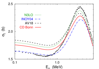
Figure 2: (Color online) Total cross section for $n\text{-}{}^{3}\mathrm{H}$ scattering as function of neutron lab energy calculated with CD Bonn (solid curve), AV18 (dashed curve), INOY04 (dash-dotted curve), and N3LO (dotted curve) potentials. Experimental data are from LABEL:~phillips:80 .

	$\varepsilon_{t}$	$\varepsilon_{\alpha}$	$a_{0}$	$a_{1}$	$\sigma_{t}$ (0)	$\sigma_{t}$ (3.5)
AV18	7.621	24.24	4.28	3.71	1.88	2.33
Nijmegen II	7.653	24.50	4.27	3.71	1.87	2.31
Nijmegen I	7.734	24.94	4.25	3.69	1.85	2.30
N3LO	7.854	25.38	4.23	3.67	1.83	2.38
CD Bonn	7.998	26.11	4.17	3.63	1.79	2.28
INOY04	8.493	29.11	4.02	3.51	1.67	2.22

Table 5: ${}^{3}\mathrm{H}$ and ${}^{4}\mathrm{He}$ binding energies $\varepsilon_{t}$ and $\varepsilon_{\alpha}$ (in MeV), $n\text{-}{}^{3}\mathrm{H}$ scattering lengths $a_{0}$ and $a_{1}$ (in fm), and $n\text{-}{}^{3}\mathrm{H}$ total cross section $\sigma_{t}$ (in barns) at $E_{n}=0$ and 3.5 MeV neutron lab energy for different $2N$ potentials.

Figure 3: Correlation between ${}^{3}\mathrm{H}$ binding energy $\varepsilon_{t}$ and $n\text{-}{}^{3}\mathrm{H}$ scattering lengths $a_{0}$ and $a_{1}$. The predictions for AV18 (diamonds), N3LO (triangles), CD Bonn (circles), and INOY04 (squares) are shown. The experimental data are from LABEL:~seagrave:80 (open circles), LABEL:~rauch:85 (open triangles), and LABEL:~hale:90a (open squares).

In Fig. 4 we show the differential cross section $d\sigma/d\Omega$ and the neutron analyzing power $A_{y}$ for $n\text{-}{}^{3}\mathrm{H}$ scattering at neutron lab energies of 1, 2, 3.5, and 6 MeV. In order to get fully converged results we take into account all $n\text{-}{}^{3}\mathrm{H}$ channel states with orbital angular momentum $L\leq 3$. The predictions of the four potentials differ mostly at forward and backward angles for the differential cross section and around the peak for the analyzing power. It is not obvious to us that the disagreement with the total cross section data shown in Fig. 2 is compatible with the discrepancies we observe relative to the differential cross section data. Therefore it would be recommended that some of the experiments be repeated at specific energies and $A_{y}$ measured in order to further understand the implications of the $2N$ force models.

One important observation that comes out of these calculations is the increased sensitivity of $4N$ observables to changes in the $2N$ interaction. The variations due to the $2N$ potential at the maximum of $n\text{-}{}^{3}\mathrm{H}$ $A_{y}$ lead to about 16% fluctuations which are larger than the 10% fluctuations observed at the peak of $A_{y}$ in low energy $n\text{-}d$ scattering. This indicates that the $4N$ system is more sensitive to off-shell differences of the $2N$ force than the $3N$ system.

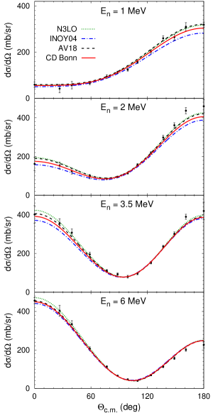
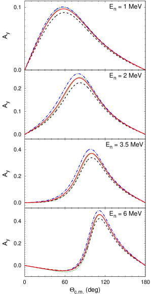
Figure 4: (Color online) Differential cross section and neutron analyzing power for $n\text{-}{}^{3}\mathrm{H}$ scattering at $E_{n}=1$, 2, 3.5, and 6 MeV neutron lab energies as functions of c.m. scattering angle. Curves as in Fig. 2. Experimental data are from LABEL:~seagrave:60 .

Finally, in Table 6 we investigate the possible correlations between the $A_{y}$-puzzle in low energy $n\text{-}d$ scattering and the underestimation of $\sigma_{t}$ in $n\text{-}{}^{3}\mathrm{H}$ scattering in the resonance region. The experimental data for $A_{y}$ in $n\text{-}d$ scattering can be accounted for by a calculation with modified interactions in $2N$ ${}^{3}P_{I}$ waves tornow:98a ; doleschall:04a . We use two models. The first one, AV18’, is taken from Ref. tornow:98a ; it corresponds to the AV18 potential that in ${}^{3}P_{I}$ waves is multiplied by strength factors 0.96, 0.98, and 1.06 for $I=0$, 1, and 2, respectively. The second one, INOY04’, is taken from Ref. doleschall:04a and differs from INOY04 by ${}^{3}P_{I}$ wave parameters. Although both modified potentials provide quite satisfactory description of vector analyzing powers in low energy $n\text{-}d$ scattering, they are incompatible with present day $2N$ data basis. E.g., the ${\chi}^{2}/\mathrm{datum}$ values with respect to the $pp$ data, estimated using the Nijmegen error matrix stoks:93a , i.e., by comparing to the Nijmegen phase shifts rather than to data directly, are 3.5 for INOY04’ and 4.4 for AV18’ potentials. However, those modifications of the potentials are unable to resolve the $\sigma_{t}$ discrepancy in $n\text{-}{}^{3}\mathrm{H}$ scattering. The $\sigma_{t}$ is slightly increased for AV18’ but it gets even lower for INOY04’, indicating that $\sigma_{t}$ depends on the $2N$ ${}^{3}P_{I}$ wave interaction in a different way than the $A_{y}$ in the $n\text{-}d$ scattering.

	$0^{+}\;(^{1}S_{0})$	$0^{-}\;(^{3}P_{0})$	$1^{+}\;(^{3}S_{1})$	$1^{-}\;(^{3}P_{1})$	$1^{-}\;(^{1}P_{1})$	$1^{-}\;(\epsilon)$	$2^{-}\;(^{3}P_{2})$	$\sigma_{t}$
AV18	-66.12	20.75	-58.48	40.09	20.73	-44.50	42.51	2.331
AV18’	-66.06	20.46	-58.39	40.50	20.86	-44.70	43.82	2.375
INOY04	-62.91	16.73	-56.00	38.75	19.47	-44.55	42.13	2.216
INOY04’	-63.04	15.67	-56.16	37.41	19.06	-43.06	42.21	2.191

Table 6: $n\text{-}{}^{3}\mathrm{H}$ phase shifts, $1^{-}$ mixing parameter $\epsilon$, and total cross section $\sigma_{t}$ at $E_{n}=3.5$ MeV for original AV18 and INOY04 potentials and their versions AV18’ and INOY04’ with modified $P$-waves.

IV Conclusions

In the present paper we developed a new numerical approach to solve four-nucleon scattering equations in momentum-space. The method uses no uncontrolled approximations, is numerically very efficient and therefore can include very large number of partial waves, thereby yielding well converged and very precise results. The developed approach is applied to $n\text{-}{}^{3}\mathrm{H}$ scattering below three-body breakup threshold. The calculations with various realistic $2N$ potentials underestimate the total $n\text{-}{}^{3}\mathrm{H}$ cross section data in the resonance region as already found by other groups. However, probably due to the inclusion of more partial waves, the numbers we get are slightly higher and closer to the data; they also depend on the choice of the $2N$ potential. The new results also show that $4N$ observables are more sensitive than $3N$ observables to the off-shell nature of the $2N$ interaction. Furthermore, the modifications that are required to introduce at the level of the ${}^{3}P_{I}$ $2N$ partial waves to remove the discrepancies in $n\text{-}d$ $A_{y}$ at low energy, do not remove the disagreement observed in the total $n\text{-}{}^{3}\mathrm{H}$ cross section around $E_{n}=3.5$ MeV. Finally, to understand the compatibility between existing $n\text{-}{}^{3}\mathrm{H}$ total and differential cross section data it would be advisable to repeat some of those experiments at specific energies.

Appendix A

As mentioned in Section III we present here our results for the binding energy of ${}^{4}\mathrm{He}$ and $n\text{-}{}^{3}\mathrm{H}$ phase shifts obtained with Mafliet-Tjon potential as well as the numerical stability check of our results. In Table 7 we show the $\alpha$ particle binding energy for increasing number of $2N$ partial waves and compare with previous works. Results with AV8’ are calculated without the Coulomb interaction in order to compare with Ref. kamada:01a . On the other hand calculations from Ref. nogga:02a ; viviani:06a with CD Bonn include coupling between total isospin $T=0,\,1$ and 2 states while we consider only $T=0$. In contrast to our scattering calculations, here we perform the isospin averaging not for the t-matrix but for the potential like it has been done in calculations of Ref. lazauskas:04a . Overall these results indicate that our algorithm is accurate and reliable.

	$I\leq$ 1	$I\leq$ 2	$I\leq$ 3	$I\leq$ 4	$I\leq$ 5	$I\leq$ 6	Other work: Refs. nogga:02a ; kamada:01a ; lazauskas:04a ; viviani:06a
AV8’	23.08	25.16	25.69	25.85	25.90	25.91	25.90 - 25.94
AV18	22.30	23.75	24.15	24.20	24.23	24.24	24.22 - 24.25
CD Bonn	25.03	25.95	26.07	26.10	26.11	26.11	26.13 - 26.16
INOY04	28.68	29.09	29.10	29.11	29.11	29.11	29.11

Table 7: ${}^{4}\mathrm{He}$ Binding Energy (MeV) for increasing number of $2N$ partial waves characterized by maximal total angular momentum $I$.

	$L=0$, $S=0$	$L=1$, $S=0$	$L=2$, $S=0$	$L=0$, $S=1$	$L=1$, $S=1$	$L=2$, $S=1$
$E_{n}=2.0$ MeV	50.93	17.19	-0.37	-45.65	22.56	-0.57
Ref. lazauskas:phd	51.1	17.2	-0.37	-45.8	22.6	-0.58
$E_{n}=3.5$ MeV	-64.53	28.00	-1.39	-58.17	40.51	-0.94
Ref. lazauskas:phd	-64.6	28.0	-1.40	-58.2	40.5	-0.89
$E_{n}=5.0$ MeV	-74.33	34.06	-2.17	-67.30	50.56	-1.53
Ref. lazauskas:phd	-74.4	34.0	-2.24	-67.4	50.5	-1.59

Table 8: $n\text{-}{}^{3}\mathrm{H}$ phase shifts at different neutron lab energies for the Mafliet-Tjon potential.

For $n\text{-}{}^{3}\mathrm{H}$ scattering we compare in Table 8 the results of our calculations with those of the Grenoble group lazauskas:phd . Again our phase shifts agree within a few tenth of a degree or better leading to identical total cross sections over a wide range of energies.

$N_{k}$	$0^{+}\;(^{1}S_{0})$	$0^{-}\;(^{3}P_{0})$	$1^{+}\;(^{3}S_{1})$	$1^{-}\;(^{3}P_{1})$	$1^{-}\;(^{1}P_{1})$	$1^{-}\;(\epsilon)$	$2^{-}\;(^{3}P_{2})$	$\sigma_{t}$
14	-70.03	23.78	-62.01	43.49	22.35	-44.58	46.93	2.290
15	-69.57	23.57	-61.61	43.64	22.40	-44.72	47.18	2.292
16	-69.43	23.51	-61.51	43.63	22.38	-44.75	47.19	2.290
18	-69.72	23.66	-61.76	43.55	22.39	-44.67	47.03	2.289
20	-69.63	23.62	-61.69	43.54	22.38	-44.69	47.03	2.288
22	-69.68	23.64	-61.73	43.53	22.39	-44.68	47.01	2.288
24	-69.66	23.64	-61.73	43.53	22.39	-44.68	47.00	2.288
25	-69.67	23.64	-61.73	43.53	22.39	-44.68	47.00	2.288

Table 9: $n\text{-}{}^{3}\mathrm{H}$ phase shifts, $1^{-}$ mixing parameter $\epsilon$, and the total cross section $\sigma_{t}$ at $E_{n}=4$ MeV for increasing number of meshpoints $N_{k}$ for the momenta $k_{x}$, $k_{y}$, and $k_{z}$. The $2N$ potential is AV18.

In Table 9 we demonstrate the stability of our results increasing the number $N_{k}$ of momentum meshpoints. All calculations use AV18 potential with $2N$ partial waves $I\leq 4+{}^{3}G_{5}$, $l_{y},\,l_{z}\leq 4$ and $J\leq\frac{9}{2}$. The results with $N_{k}=20$ which is the choice for calculations of Tables 1 — 3 are converged to better than 0.05 deg for all phase shifts.

References

- (1) W. Glöckle, H. Witała, D. Hüber, H. Kamada, and J. Golak, Phys. Rep. 274, 107 (1996).
- (2) J. Golak, R. Skibiński, H. Witała, W. Glöckle, A. Nogga, and H. Kamada, Phys. Rep. 415, 89 (2005).
- (3) A. Kievsky, M. Viviani, and S. Rosati, Phys. Rev. C 64, 024002 (2001).
- (4) A. C. Fonseca, Phys. Rev. Lett. 83, 4021 (1999).
- (5) A. C. Fonseca, G. Hale, and J. Haidenbauer, Few-Body Syst. 31, 139 (2002).
- (6) P. Grassberger and W. Sandhas, Nucl. Phys. B2, 181 (1967); E. O. Alt, P. Grassberger, and W. Sandhas, JINR report No. E4-6688 (1972).
- (7) T. W. Phillips, B. L. Berman, and J. D. Seagrave, Phys. Rev. C 22, 384 (1980).
- (8) F. Cieselski, J. Carbonell, and C. Gignoux, Phys. Lett. B447, 199 (1999); J. Carbonell, Few-Body Syst. Suppl. 12, 439 (2000).
- (9) O. A. Yakubovsky, Yad. Fiz. 5, 1312 (1967) [Sov. J. Nucl. Phys. 5, 937 (1967)].
- (10) R. Lazauskas and J. Carbonell, Phys. Rev. C 70, 044002 (2004).
- (11) R. Lazauskas, J. Carbonell, A. C. Fonseca, M. Viviani, A. Kievsky, and S. Rosati, Phys. Rev. C 71, 034004 (2005).
- (12) J. A. Tjon, Phys. Lett. B56, 217 (1975).
- (13) M. Viviani, S. Rosati, and A. Kievsky, Phys. Rev. Lett. 81, 1580 (1998).
- (14) M. Viviani, A. Kievsky, S. Rosati, E. A. George, and L. D. Knutson, Phys. Rev. Lett. 86, 3739 (2001).
- (15) A. Deltuva, A. C. Fonseca, and P. U. Sauer, Phys. Rev. C 71, 054005 (2005).
- (16) A. Deltuva, A. C. Fonseca, and P. U. Sauer, Phys. Rev. Lett. 95, 092301 (2005).
- (17) A. Deltuva, A. C. Fonseca, and P. U. Sauer, Phys. Rev. C 72, 054004 (2005).
- (18) A. Deltuva and A. C. Fonseca, in Proceedings of the 18th International IUPAP Conference on Few-Body Problems in Physics, Santos, 2006, nucl-th/0611013.
- (19) A. C. Fonseca, in Models and Methods in Few-Body Physics, Lecture Notes in Physics 273, p. 161, edited by L. S. Fereira, A. C. Fonseca, and L. Streit (Springer Verlag, Heidelberg, 1987).
- (20) H. Kamada and W. Glöckle, Nucl. Phys. A548, 205 (1992).
- (21) W. Glöckle and H. Kamada, Phys. Rev. Lett. 71, 971 (1993).
- (22) G. A. Baker, Essentials of Padé Approximants (Academic Press, New York, 1975).
- (23) K. Chmielewski, A. Deltuva, A. C. Fonseca, S. Nemoto, and P. U. Sauer, Phys. Rev. C 67, 014002 (2003).
- (24) A. Deltuva, Ph.D. thesis, University of Hannover, 2003, http://edok01.tib.uni-hannover.de/edoks/e01dh03/374454701.pdf.
- (25) A. Deltuva, K. Chmielewski, and P. U. Sauer, Phys. Rev. C 67, 034001 (2003).
- (26) C. de Boor, A Practical Guide to Splines (Springer Verlag, New York, 1978).
- (27) W. Glöckle, G. Hasberg, and A. R. Neghabian, Z. Phys. A305, 217 (1982).
- (28) W. H. Press, B. P. Flannery, S. A. Teukolsky, and W. T. Vetterling, Numerical Recipes (Cambridge University Press, Cambridge, 1989).
- (29) A. Nogga, H. Kamada, W. Glöckle, and B. R. Barrett, Phys. Rev. C 65, 054003 (2002).
- (30) H. Kamada et al., Phys. Rev. C 64, 044001 (2001).
- (31) M. Viviani, L. E. Marcucci, S. Rosati, A. Kievsky, and L. Girlanda, Few-Body Syst. 39, 159 (2006).
- (32) R. Lazauskas, Ph.D. thesis, University of Grenoble, 2003; private communication.
- (33) R. B. Wiringa, V. G. J. Stoks, and R. Schiavilla, Phys. Rev. C 51, 38 (1995).
- (34) R. Machleidt, Phys. Rev. C 63, 024001 (2001).
- (35) V. G. J. Stoks, R. A. M. Klomp, C. P. F. Terheggen, and J. J. de Swart, Phys. Rev. C 49, 2950 (1994).
- (36) P. Doleschall, Phys. Rev. C 69, 054001 (2004); private communication.
- (37) D. R. Entem and R. Machleidt, Phys. Rev. C 68, 041001(R) (2003).
- (38) J. D. Seagrave, B. L. Berman, and T. W. Phillips, Phys. Lett. B91, 200 (1980).
- (39) H. Rauch, D. Tuppinger, H. Wölwitsch, and T. Wroblewski, Phys. Lett. B165, 39 (1985).
- (40) G. M. Hale, D. C. Dodder, J. D. Seagrave, B. L. Berman, and T. W. Phillips, Phys. Rev. C 42, 438 (1990).
- (41) J. D. Seagrave, L. Cranberg, and J. E. Simmons, Phys. Rev. 119, 1981 (1960).
- (42) W. Tornow, H. Witała, and A. Kievsky, Phys. Rev. C 57, 555 (1998).
- (43) V. Stoks and J. J. de Swart, Phys. Rev. C 47, 761 (1993).