Abstract

The $(ed\rightarrow enp)$ process in the frame of the Bethe-Salpeter approach with a separable kernel of the Nucleon-Nucleon (NN) interaction was considered. This conception keeps the covariance of description of the process. Special attention was devoted to a contribution of the $D$-states of the deuteron in the cross section of the electrodisintegration. It was shown that the spectator particle (neutron) plays an important role. The factorization of a cross section of this reaction in the impulse approximation was checked by analytical and numerical calculations.

1.  Introduction

Study of static and dynamic electromagnetic properties of light nuclei and, especially, the deuteron enables more deeply to understand a nature of strong interactions and, in particular, nucleon-nucleon interactions. At high energies considerations of a nucleus as a nucleon system are not well justified. For this reason the problems to study non-nucleonic degrees of freedom (mesons, $\Delta$-isobars, quark admixtures etc.) in an intermediate energies region are widely discussed. However, in spite of it significant progress was achieved on this way relativistic effects (which a priori are very important at large transfer momenta) are needed to include in the consideration.

Other actively discussed problem is the extraction from experiments with light nuclei of the information about a structure of bounded nucleons. It requires to take into account relativistic kinematics of the reaction and dynamics of interaction. So the construction of a covariant approach and detailed analysis of relativistic effects in electromagnetic reactions with light nuclei are very important and interesting.

The electrodisintegration of the deuteron at the threshold has been of interest of an investigation for a long time [1]-[6]. The reason is that the electrodisintegration is an essential instrument for study a structure of a two-nucleon system. First of all it is an electromagnetic structure. The deuteron has been used as a neutron target to get the information about neutron electromagnetic form factors. During last 20 years it has also been used to receive constraints on available realistic NN potentials. Analyzing of the electrodisintegration process we can clarify the role of non-nucleonic degrees of freedom. The non-nucleonic effects are often important in few-body systems. And the deuteron is one of convenient candidates because complete calculations can in principle be performed.

First experiments were carried out at low transfer momenta but more modern experiments [7]-[12] performed at high momenta have opened many new questions in a region where relativistic effects are important. The experimental results on the differential cross section derived from $(ed\rightarrow enp)$ reaction are available up to a momentum transfer of about 1 GeV. This situation is very good for investigation of the deuteron structure at short distances with the allowance for some exotic effects which have not been earlier important. First of all these are the quark degrees of freedom (see [13], [14], for instance), but formerly it is necessary to take into account relativistic effects.

Bethe-Salpeter (BS) approach [15] can give a possibility to consider relativistic effects by consistent way [16]. In the paper the deuteron electrodisintegration within the covariant BS approach with the separable Graz II interaction kernel is presented. The exclusive differential cross section is calculated in the plane wave relativistic impulse approximation.

The paper is organized as follows. In section 2 the relativistic kinematics of the reaction and formulae for the cross section are considered. The BS amplitude is presented in section 3. The hadron current in the BS formalism is defined in section 4. Factorization of the cross section is discussed in section 5. Then the results of our numerical calculations are presented in section 6. Finally the discussion of the results is performed and further plans are outlined.

2.  Cross section and kinematics

Let us consider the relativistic kinematics of the exclusive electrodisintegration of the deuteron. The initial electron $l=(E,{\mbox{\boldmath$l$}})$ collides with the deuteron in rest frame $K=(M_{d},{\mbox{\boldmath$0$}})$ ($M_{d}$ is a mass of the deuteron). And there are three particles in the final state, i.e. electron $l^{\prime}=(E^{\prime},{\mbox{\boldmath$l$}}^{\prime})$ and pair of proton and neutron. In one photon approximation (we also neglect the electron mass) a squared momentum of the virtual photon $q=(\omega,{\mbox{\boldmath$q$}})$ can be expressed via electron scattering angle $\theta$

$$q^{2}=-Q^{2}=(l-l^{\prime})^{2}=\omega^{2}-{\mbox{\boldmath$q$}}^{2}=-4|{\mbox{\boldmath$l$}}||{\mbox{\boldmath$l$}}^{\prime}|\sin^{2}\frac{\theta}{2}.$$ (1)

$np$-pair is described by the invariant mass $s=P^{2}=(p_{p}+p_{n})^{2}$ which can be expressed through components of photon 4-impulse:

$$s=M_{d}^{2}+2M_{d}\omega+q^{2}.$$ (2)

Lorentz invariant matrix element of the reaction (see Fig. 1) can be written as a product of lepton and hadron currents

$$M_{fi}=-\imath e^{2}(2\pi)^{4}\delta^{(4)}(K-P+q)\hskip 170.71652pt$$

$$\times<l^{\prime},s_{e}^{\prime}|j^{\mu}|l,s_{e}>\frac{1}{q^{2}}<np:(P,Sm_{S})|J_{\mu}|d:(K,M)>,$$ (3)

where $<l^{\prime},s_{e}^{\prime}|j^{\mu}|l,s_{e}>=\bar{u}(l^{\prime},s_{e}^{\prime})\gamma^{\mu}u(l,s_{e})$ is an electromagnetic current (EM). The initial (final) electron is described by Dirac spinor $u(l,s_{e})$ ($\bar{u}(l^{\prime},s_{e}^{\prime})$). The hadron current $<np:(P,Sm_{S})|J_{\mu}|d:(K,M)>$ is a transition matrix element from the initial deuteron $|d:(K,M)>$ with total momentum $K$, projection $M$ to the final $np$-pair $|np:(P,Sm_{S})>$ with total momentum $P$ and spin $S$, projection $m_{S}$.

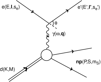
Figure 1: One photon approximation.

Thus the unpolarized cross section of the electrodisintegration of the deuteron can be easily written as

$$\frac{d^{5}\sigma}{dE^{\prime}d\Omega^{\prime}d\Omega_{\mbox{\boldmath$p$}}}=\frac{\alpha^{2}}{8M_{d}(2\pi)^{3}}\frac{|{\mbox{\boldmath$l$}}^{\prime}|}{|{\mbox{\boldmath$l$}}|}\frac{\sqrt{s}}{q^{4}}{R}\,l^{\mu\nu}W_{\mu\nu},$$ (4)

where the factor $R$ connects the final proton angle in the center of mass system (C.M.S.) (where the $np$-pair is rest) with the same in the laboratory system (L.S.):

$$R=\frac{{\mbox{\boldmath$p$}}^{2}}{\sqrt{1+\eta}|{\mbox{\boldmath$p$}}|-e_{\mbox{\boldmath$p$}}\sqrt{\eta}\cos\theta_{{\mbox{\boldmath$p$}}}}.$$ (5)

Here $p$ is a momentum of the final proton in L.S., $e_{\mbox{\boldmath$p$}}=\sqrt{{\mbox{\boldmath$p$}}^{2}+m^{2}}$, $\theta_{\mbox{\boldmath$p$}}$ is an angle between the final proton and $Z$-axis, $m$ is a nucleon mass, and $\eta={\mbox{\boldmath$q$}}^{2}/s$.

Tensor of unpolarized leptons in (4) is expressed as

$$l_{\mu\nu}=\frac{1}{2}\sum_{s_{e}\,s_{e}^{\prime}}<l^{\prime},s_{e}^{\prime}|{{j_{\mu}}^{{\dagger}}}|l,s_{e}><l,s_{e}|j_{\nu}|l^{\prime},s_{e}^{\prime}>=2(l^{\prime}_{\mu}l_{\nu}+l^{\prime}_{\nu}l_{\mu})+g_{\mu\nu}q^{2}$$ (6)

and hadron tensor can be written as

$$W_{\mu\nu}=\frac{1}{3}\sum_{MSm_{s}}<d:(K,M)|{J_{\mu}}^{{\dagger}}|np:(P,Sm_{S})><np:(P,Sm_{S})|J_{\nu}|d:(K,M)>.$$ (7)

In order to average on initial and sum on final states let us introduce a helicity tensor which can be directly connected with structure functions (see, for example [1],[4],[6]). These quantities allow to calculate polarization and asymmetry observables easily and may be necessary in future (we didn’t calculate them in this work). Keeping in mind the Hermitian properties of the lepton and the hadron tensors the cross section can be rewritten as

$$\frac{d^{5}\sigma}{dE^{\prime}d\Omega^{\prime}d\Omega_{\mbox{\boldmath$p$}}}=\frac{\sigma_{Mott}}{8M_{d}(2\pi)^{3}}{\sqrt{s}}{R}\hskip 199.16928pt$$

$$\times\left[l^{0}_{00}W_{00}+l^{0}_{++}(W_{++}+W_{--})+l^{0}_{+-}2{\mbox{\rm Re}}W_{+-}-l^{0}_{0+}2{\mbox{\rm Re}}(W_{0+}-W_{0-})\right],$$ (8)

where $\sigma_{Mott}=(\alpha\cos\frac{\theta}{2}/2E\sin^{2}\frac{\theta}{2})^{2}$ is Mott cross section for point-like particles and

$$l_{00}^{0}=\frac{Q^{2}}{{\mbox{\boldmath$q$}}^{2}},\quad l_{0+}^{0}=\frac{Q}{|{\mbox{\boldmath$q$}}|\sqrt{2}}\sqrt{\frac{Q^{2}}{{\mbox{\boldmath$q$}}^{2}}+\textmd{tg}^{2}\frac{\theta}{2}},\quad l_{++}^{0}=\frac{1}{2}\textmd{tg}^{2}\frac{\theta}{2}+\frac{Q^{2}}{4{\mbox{\boldmath$q$}}^{2}},\quad l_{+-}^{0}=-\frac{Q^{2}}{2{\mbox{\boldmath$q$}}^{2}}.$$ (9)

So the calculation of the cross section (8) comes to the calculation of the hadron tensor $W_{\mu\nu}$ which describes the NN interaction and is a subject of our investigation.

3.  Bethe-Salpeter Amplitude of the Deuteron

In the Bethe-Salpeter approach (BSA) the deuteron is a bound system which can be described by the amplitude $\Phi_{M}(k;K)$ of the equation

$$\Phi_{M\,\alpha\beta}(k;K)=\imath S^{(1)}_{\alpha\eta}\left(\frac{K}{2}+k\right)S^{(2)}_{\beta\rho}\left(\frac{K}{2}-k\right)\int\frac{d^{4}k^{\prime}}{(2\pi)^{4}}V_{\eta\rho,\epsilon\lambda}(k,k^{\prime};K)\Phi_{M\,\epsilon\lambda}(k^{\prime};K),$$ (10)

here $S^{(\ell)}(K/2-(-1)^{\ell}k)$ is a propagator of the $\ell$-th nucleon, $V(k,k^{\prime};K)$ is a kernel of a NN interaction (Greek letters means spinor indexes). The amplitude of the deuteron in rest frame can be expanded through two-nucleon relativistic states $|aM\rangle\equiv|\pi,\,{}^{2S+1}L_{J}^{\rho}M\rangle$:

$$\Phi_{M}(k;K)=\sum_{a}\phi_{a}(k_{0},|{\mbox{\boldmath$k$}}|){\cal Y}_{aM}({\mbox{\boldmath$k$}}),$$ (11)

where $S$ denotes a total spin of the system, $L$ is an orbital angular momentum, $J$ is a total angular momentum with a projection $M$. Quantum number $\rho$ counts positive- and negative-energy states, $\pi$ marks the parity of the state; $\phi_{a}(k_{0},|{\mbox{\boldmath$k$}}|)$ is the radial part of the BS amplitude. The spin-angular part ${\cal Y}_{aM}({\mbox{\boldmath$k$}})$) is

$${\cal Y}_{aM}({\mbox{\boldmath$k$}})U_{C}=\hskip 273.14645pt$$

$$\imath^{L}\sum_{m_{L}m_{S}m_{1}m_{2}\rho_{1}\rho_{2}}C_{\frac{1}{2}\rho_{1}\frac{1}{2}\rho_{2}}^{S_{\rho}{\rho}}C_{Lm_{L}Sm_{S}}^{JM}C_{\frac{1}{2}m_{1}\frac{1}{2}m_{2}}^{Sm_{S}}Y_{L{m_{L}}}({\mbox{\boldmath$k$}}){u^{\rho_{1}}_{m_{1}}}({\mbox{\boldmath$p$}}){{u^{\rho_{2}}_{m_{2}}}}^{T}(-{\mbox{\boldmath$k$}}).$$ (12)

Using partial wave decomposition (11) we can write the decomposed Bethe-Salpeter equation for the radial part of the BSA

$$\phi_{a}(k_{0},|{\mbox{\boldmath$k$}}|)=S_{a}(k_{0},|{\mbox{\boldmath$k$}}|;s)\int dk_{0}^{\prime}\int{{\mbox{\boldmath$k$}}^{\prime}}^{2}d|{\mbox{\boldmath$k$}}^{\prime}|\sum\limits_{b}V_{ab}(k_{0},|{\mbox{\boldmath$k$}}|,k_{0}^{\prime},|{\mbox{\boldmath$k$}}^{\prime}|;s)\phi_{b}(k_{0}^{\prime},|{\mbox{\boldmath$k$}}^{\prime}|).$$ (13)

Then taking into account separable anzats for the rank $N$ kernel of interaction

$$V_{ab}(k_{0},|{\mbox{\boldmath$k$}}|,k_{0}^{\prime},|{\mbox{\boldmath$k$}}^{\prime}|;s)=\sum\limits_{i,j=1}^{N}\lambda_{ij}\,g_{i}^{a}(k_{0},|{\mbox{\boldmath$k$}}|)\,g_{j}^{b}(k_{0}^{\prime},|{\mbox{\boldmath$k$}}^{\prime}|),\qquad\lambda_{ij}=\lambda_{ji},$$ (14)

we can find a solution of the BS equation (13) in the following form

$$\phi_{a}(k_{0},|{\mbox{\boldmath$k$}}|)=\sum\limits_{i,j=1}^{N}S_{a}(k_{0},|{\mbox{\boldmath$k$}}|;s)\,\lambda_{ij}\,g_{i}^{a}(k_{0},|{\mbox{\boldmath$k$}}|)\,c_{j}(s).$$ (15)

Here $\lambda_{ij}$ are fitting parameters, $g_{i}^{a}(k_{0},|{\mbox{\boldmath$k$}}|)$ are trial functions. The coefficients $c_{j}(s)$ satisfy the following system of homogeneous equations

$$c_{i}(s)\,-\,\sum\limits_{k,j=1}^{N}\,h_{ik}(s)\,\lambda_{kj}\,c_{j}(s)\,=\,0,$$ (16)

where $h_{ik}(s)$ are defined by the integral

$$h_{ik}(s)=\frac{\imath}{2\pi^{2}}\sum\limits_{a}\int\,dk_{0}\,\int{\mbox{\boldmath$k$}}^{2}\,d|{\mbox{\boldmath$k$}}|\,S_{a}(k_{0},|{\mbox{\boldmath$k$}}|;s)\,g_{i}^{a}(k_{0},|{\mbox{\boldmath$k$}}|)\,g_{k}^{a}(k_{0},|{\mbox{\boldmath$k$}}|).$$ (17)

Using the covariant separable Graz II rank III kernel of interaction [16] we can find $\lambda_{ij}$ (see Table 1) from an analysis of the experimental data for the deuteron characteristics (phase shifts, binding energy, length of scattering etc.).

Table 1: Parameters of the covariant separable Graz II kernel

$$\gamma_{1}$$ 28.69550 GeV^-2 2.718930 10^-4 GeV⁶

64.9803 GeV^-2 -7.16735 10^-2 GeV⁴

2.31384 10^-1 GeV -1.51744 GeV⁶

5.21705 GeV 16.52393 GeV²

7.94907 GeV 0.28606 GeV⁴

1.57512 GeV 3.48589 GeV⁶

It is necessary to remark that here we took into account the positive-energy states (${}^{3}S_{1}^{+}$, ${}^{3}D_{1}^{+}$) only

$$g_{1}^{{}^{3}S_{1}^{+}}(k_{0},|{\mbox{\boldmath$k$}}|)=\frac{1-\gamma_{1}(k_{0}^{2}-{\mbox{\boldmath$k$}}^{2})}{(k_{0}^{2}-{\mbox{\boldmath$k$}}^{2}-\beta_{11}^{2})^{2}}$$ (18)

$$g_{2}^{{}^{3}S_{1}^{+}}(k_{0},|{\mbox{\boldmath$k$}}|)=-\frac{(k_{0}^{2}-{\mbox{\boldmath$k$}}^{2})}{(k_{0}^{2}-{\mbox{\boldmath$k$}}^{2}-\beta_{12}^{2})^{2}}$$ (19)

$$g_{3}^{{}^{3}D_{1}^{+}}(k_{0},|{\mbox{\boldmath$k$}}|)=\frac{(k_{0}^{2}-{\mbox{\boldmath$k$}}^{2})(1-\gamma_{2}(k_{0}^{2}-{\mbox{\boldmath$k$}}^{2}))}{(k_{0}^{2}-{\mbox{\boldmath$k$}}^{2}-\beta_{21}^{2})(k_{0}^{2}-{\mbox{\boldmath$k$}}^{2}-\beta_{22}^{2})^{2}}$$ (20)

$$g_{1}^{{}^{3}D_{1}^{+}}(k_{0},|{\mbox{\boldmath$k$}}|)=g_{2}^{{}^{3}D_{1}^{+}}(k_{0},|{\mbox{\boldmath$k$}}|)=g_{3}^{{}^{3}S_{1}^{+}}(k_{0},|{\mbox{\boldmath$k$}}|)\equiv 0.$$ (21)

In our calculation it is more convenient to use the BS vertex $\Gamma_{M}$ which is related with the BS amplitude by simple expression. For full functions

$$\Phi_{M}(k;K)=S^{(1)}\left(\frac{K}{2}+k\right)S^{(2)}\left(\frac{K}{2}-k\right)\Gamma_{M}(k;K),$$ (22)

and for their radial parts

$$\phi_{a}(k_{0},|{\mbox{\boldmath$k$}}|)=\sum_{b}S_{ab}(k_{0},|{\mbox{\boldmath$k$}}|;s)g_{b}(k_{0},|{\mbox{\boldmath$k$}}|),$$ (23)

here we omitted spinor indexes for simplicity. $S_{ab}$ is a nucleon propagator which is diagonal for positive-energy partial parts

$$S_{++}(k_{0},|{\mbox{\boldmath$k$}}|;s)=1/\left[\left(\sqrt{s}/{2}+k_{0}-e_{\mbox{\boldmath$k$}}\right)\left(\sqrt{s}/{2}-k_{0}-e_{\mbox{\boldmath$k$}}\right)\right].$$ (24)

4.  Hadron Electromagnetic Current

Let us write the matrix element of the hadron electromagnetic current with the BS amplitude using Mandelstam technique [17]

$$<np:(P,Sm_{S})|J_{\mu}|d:(K,M)>=\hskip 199.16928pt$$

$$\imath\int\frac{d^{4}p}{(2\pi)^{4}}\,\frac{d^{4}k}{(2\pi)^{4}}\,\bar{\chi}_{Sm_{s}}(p;p^{*},P)\,\Lambda_{\mu}(p,k;P,K)\,\Phi_{M}(k;K).$$ (25)

Here $p^{*}$ is the relative 4-momentum of the $np$-pair (nucleons are on-mass-shell), $Pp^{*}=0$, and ${{\mbox{\boldmath$p$}}^{*}}^{2}=s/4-m^{2}$.

We consider the process of the electrodisintegration of the deuteron in RIA (see Fig. 2). In our further calculation only one-body currents are taken into account

$$\Lambda^{[1]}_{\mu}(p,k;P,K)=\imath(2\pi)^{4}\left\{\delta^{(4)}(p-k-\frac{q}{2})\Gamma^{(1)}_{\mu}\left(\frac{P}{2}+p,\frac{K}{2}+k\right){S^{(2)}\left(\frac{P}{2}-p\right)}^{-1}\right.\hskip 14.22636pt$$

$$\left.+\delta^{(4)}(p-k+\frac{q}{2})\Gamma^{(2)}_{\mu}\left(\frac{P}{2}-p,\frac{K}{2}-k\right){S^{(1)}\left(\frac{P}{2}+p\right)}^{-1}\right\}$$ (26)

(here the total and relative momenta are introduced: $P=p_{1}+p_{2},K=k_{1}+k_{2},k=\frac{1}{2}(k_{1}-k_{2}),p=\frac{1}{2}(p_{1}-p_{2})$).

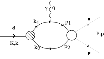
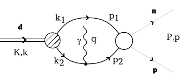
Figure 2: Relativistic impulse approximation.

In this case the matrix element of the hadron current has the following form

$$<np:(P,Sm_{S})|J_{\mu}|d:(K,M)>=\imath\sum_{\ell=1,2}\int\frac{d^{4}p}{(2\pi)^{4}}\ \bar{\chi}_{Sm_{S}}(p;P)$$

$$\Gamma_{\mu}^{(\ell)}(q)\ S^{(\ell)}\left(\frac{P}{2}-(-1)^{\ell}p-q\right)\ \Gamma_{M}\left(p+(-1)^{\ell}\frac{q}{2};K\right).$$ (27)

Note that $\gamma NN$- vertex was taken on-mass-shell

$$\Gamma_{\mu}^{(\ell)}(p^{\prime},p)\longrightarrow\Gamma^{(\ell)}_{\mu}(q)=\gamma_{\mu}F^{(\ell)}_{1}(q^{2})-\frac{1}{4m}\left(\gamma_{\mu}\hat{q}-\hat{q}\gamma_{\mu}\right)F^{(\ell)}_{2}(q^{2}).$$ (28)

Here $F^{(\ell)}_{1}$ ($F^{(\ell)}_{2}$) - Dirac (Pauli) form factor of the nucleon which obeys the next normalization conditions

$$F^{(1)}_{1}(0)=1,\qquad F^{(1)}_{2}(0)=\varkappa_{p},$$

$$F^{(2)}_{1}(0)=0,\qquad F^{(2)}_{2}(0)=\varkappa_{n},$$ (29)

$\varkappa_{p}$ ($\varkappa_{n}$) is the anomalous proton (neutron) magnetic moment.

It should be mentioned that we neglect a final state interaction (FSI) (it is a subject of future calculations).

$$\bar{\chi}^{(0)}_{Sm_{s}}(p;p^{*},P)=(2\pi)^{4}\,\delta^{(4)}(p-p^{*})\,\bar{\chi}^{(0)}_{Sm_{S}}(p^{*},P)$$

$$=(2\pi)^{4}\,\delta^{(4)}(p-p^{*})\,\sum_{m_{1}m_{2}}C_{\frac{1}{2}m_{1}\frac{1}{2}m_{2}}^{Sm_{S}}\,{\bar{u}}_{m_{1}}\left(\frac{P}{2}+p\right)\,{\bar{u}}_{m_{2}}\left(\frac{P}{2}-p\right).$$ (30)

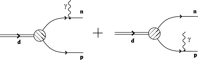
Figure 3: Plane wave approximation.

Using (30) for the final $np$-pair wave function and integrating (27) over $p$ we obtain our basic RIA expression for the hadron current

$$<np:(P,Sm_{S})|J_{\mu}|d:(K,M)>=\imath\sum_{\ell=1,2}\bar{\chi}^{(0)}_{Sm_{S}}(p^{*},P)\Gamma_{\mu}^{(\ell)}(q)$$

$$\times S^{(\ell)}\left(\frac{K}{2}-p^{*}-(-1)^{\ell}\frac{q}{2}\right)\Gamma_{M}\left(p^{*}+(-1)^{\ell}\frac{q}{2};K\right).$$ (31)

It has very simple form. And to get it we should just perform the analytical calculation of the trace. For this purpose we use the REDUCE system.

5.  Factorization of the cross section

Let us consider the electrodisintegration of the deuteron supposing that an initial lepton collides only with the proton in the deuteron and the neutron is a spectator. Then the cross section is factorized on two parts, one is connected with the contribution of the neutron as a spectator and another with a proton contribution, the latter does not have interference terms between the $S$- and $D$-states.

5.1  Nonrelativistic case

The amplitude of the process can formally be presented as a production

$${\cal M}=\chi^{+}_{m_{1}}\chi^{+}_{m_{2}}\hat{O}\Psi_{M},$$ (32)

where spinors $\chi^{+}_{m_{1}},~{}\chi^{+}_{m_{2}}$ describe the outgoing $np$-pair, $\hat{O}$ corresponds to the interaction vertex, $\Psi_{M}$ is a wave function of the deuteron. Let us note that the vertex $\hat{O}$ stands in general for any one-particle interaction, but in this paper describes $\gamma NN$-vertex.

Inserting into this expression a complete set of pair states we can get

$${\cal M}_{\mu}=\sum_{m_{1}^{\prime}}(\chi^{+}_{m_{1}}\hat{O}_{\mu}\chi_{m_{1}^{\prime}})\chi^{+}_{m_{1}^{\prime}}\chi^{+}_{m_{2}}\Psi_{M},$$ (33)

after evident transformations the hadron tensor can be written as

$$W_{\mu\nu}=\frac{1}{3}\sum_{m_{1}m_{2}M}{\cal M}_{\mu}{\cal M}_{\nu} = \frac{1}{3}\sum_{m_{1}m_{2}M}\left|\sum_{m_{1}^{\prime}}\left[\chi^{+}_{m_{1}}\hat{O}\chi_{m_{1}^{\prime}}\right]\left[\chi^{+}_{m_{1}^{\prime}}\chi^{+}_{m_{2}}\Psi_{M}\right]\right|^{2}$$

$$= \frac{1}{3}\sum_{m_{1}m_{2}M}\sum_{m_{1}^{\prime}m_{1}^{\prime\prime}}\left[\chi_{m_{1}}^{+}\hat{O}\chi_{m_{1}^{\prime}}\right]^{2}\left[\chi^{+}_{m_{1}^{\prime}}\chi_{m_{2}}^{+}\Psi_{M}\Psi^{+}_{M}\chi_{m_{2}}\chi_{m_{1}^{\prime\prime}}\right].$$

Introducing the partial-wave decomposition for the deuteron:

$$\Psi_{M}=\sum_{lms_{1}s_{2}s}C_{lm1s}^{1M}C_{\frac{1}{2}s_{1}\frac{1}{2}s_{2}}^{1s}Y_{lm}\chi_{s_{1}}\chi_{s_{2}}u_{l}$$

and transforming the second term with the help of orthogonalization properties of the spinor $\chi$ and some relations for Clebsh-Gordan coefficients we can finally obtain the factorized expression

$$W_{\mu\nu}=\frac{1}{8\pi}|A_{\mu}A^{*}_{\nu}|\sum_{l}|u_{l}|^{2},$$ (34)

where $A_{\mu}=\chi_{m_{1}}^{+}\hat{O}_{\mu}\chi_{m_{1}^{\prime}}$ is a one-body interaction part and $l$ counts partial states of the deuteron.

Thus it is seen that the cross section is proportional to the sum of squared radial parts of the deuteron wave function.

5.2  Relativistic case

In the relativistic case the matrix element of the deuteron electrodisintegration can be written schematically in the following form

$${\cal M}=\Psi_{pair}\otimes\hat{O}\otimes S\otimes\Gamma_{M},$$ (35)

where $\Psi_{pair}$ is the wave function of the $np$-pair, $\hat{O}$ is a vertex of interaction, $S$ is a propagator of the nucleon, $\Gamma_{M}$ is the vertex function of the deuteron.

Introducing the partial-wave decomposition of the deuteron vertex function in the L.S., considering the only proton interacting with a virtual photon and supposing the PWA for the final $np$-pair we can present the comprehensive expression in the following form

$${\cal M}_{\mu} = \sum_{s_{1}s_{2}}C_{\frac{1}{2}s_{1}\frac{1}{2}s_{2}}^{SM_{S}}\bar{u}^{(1)}(s_{1},{\mbox{\boldmath$p$}}_{1})\bar{u}^{(2)}(s_{2},{\mbox{\boldmath$p$}}_{2})\Gamma^{(1)}_{\mu}(q)S_{1\,+}({\mbox{\boldmath$k$}}_{1})\sum_{m_{1}^{\prime}}u^{(1)}(m_{1}^{\prime},{\mbox{\boldmath$k$}}_{1})\bar{u}^{(1)}(m_{1}^{\prime},{\mbox{\boldmath$k$}}_{1})$$

$$\times\sum_{m_{1}m_{2}lmsm_{s}}C_{lmsm_{s}}^{1M}C_{\frac{1}{2}m_{1}\frac{1}{2}m_{2}}^{sm_{s}}u^{(1)}(m_{1},-{\mbox{\boldmath$k$}}_{1})u^{(2)}(m_{2},-{\mbox{\boldmath$k$}}_{2})Y_{lm}(\hat{\mbox{\boldmath$k$}})g_{l}(k_{0},|{\mbox{\boldmath$k$}}|),$$

where $S_{1\,+}({\mbox{\boldmath$k$}}_{1})=1/(k_{10}-e_{{\mbox{\boldmath$k$}}_{1}})$ and $\Gamma^{(1)}_{\mu}(q)$ vertex is described by Eq. (28). As it was assumed above only ${}^{3}S_{1}^{+},~{}^{3}D_{1}^{+}$-states were taken into account. Using orthogonalization properties of the bispinors and some relations for Clebsh-Gordan coefficients we can write

$${\cal M}_{\mu}=\sum_{s_{1}s_{2}m_{1}lmsm_{s}}C_{\frac{1}{2}s_{1}\frac{1}{2}s_{2}}^{SM_{S}}C_{lmsm_{s}}^{1M}C_{\frac{1}{2}m_{1}\frac{1}{2}s_{2}}^{sm_{s}}Y_{lm}(\hat{\mbox{\boldmath$k$}})g_{l}(k_{0},|{\mbox{\boldmath$k$}}|)S_{1\,+}({\mbox{\boldmath$k$}}_{1})A^{(1)}_{\mu}(s_{1},{\mbox{\boldmath$p$}}_{1};m_{1},{\mbox{\boldmath$k$}}_{1}),$$

with

$$A^{(1)}_{\mu}(s_{1},{\mbox{\boldmath$p$}}_{1};m_{1},{\mbox{\boldmath$k$}}_{1})=\bar{u}^{(1)}(s_{1},{\mbox{\boldmath$p$}}_{1})\Gamma^{(1)}_{\mu}(q)u^{(1)}(m_{1},{\mbox{\boldmath$k$}}_{1}),$$ (36)

is a one-body photon-proton interaction part. Now we can derive the hadron tensor

$$W_{\mu\nu}=\frac{1}{3}\sum_{MSM_{S}}{\cal M}_{\mu}{\cal M}_{\nu}.$$

Using once more properties of the Clebsh-Gordan coefficients and Dirac spinors we obtain the expression

$$W_{\mu\nu}=C_{d}\ Sp\left\{(\hat{p}_{1}+m)\Gamma^{(1)}_{\mu}(q)(\hat{k}_{1}+m){\bar{\Gamma}^{(1)}}_{\mu}(q)\right\}$$ (37)

which involves the simply calculated trace and a function

$$C_{d}=\frac{1}{8\pi}\frac{1}{4e_{{\mbox{\boldmath$k$}}_{1}}e_{{\mbox{\boldmath$p$}}_{1}}}S_{1\,+}^{2}({\mbox{\boldmath$k$}}_{1})\sum_{l=0,2}|g_{l}(k_{0},|{\mbox{\boldmath$k$}}|)|^{2}$$

containing the structure of the deuteron. Performing the trace calculation we finally obtain the expression for the hadron tensor

$$W_{\mu\nu}=C_{d}\ \left(W^{a}_{\mu\nu}F_{1}^{2}(q^{2})+W^{b}_{\mu\nu}F_{1}(q^{2})F_{2}(q^{2})+W^{c}_{\mu\nu}F_{2}^{2}(q^{2})\right)$$ (38)

with

$$W^{a}_{\mu\nu}=4\left[p_{1\,\mu}k_{1\,\nu}+k_{1\,\mu}p_{1\,\nu}+(m^{2}-(p_{1}\cdot k_{1}))g_{\mu\nu}\right]$$ (39)

$$W^{b}_{\mu\nu}=2\left[k_{1\,\mu}q_{\nu}-q_{\mu}k_{1\,\nu}-p_{1\,\mu}q_{\nu}+q_{\mu}p_{1\,\nu}\right]$$

$$W^{c}_{\mu\nu}=\left[\left(-q^{2}m^{2}-q^{2}(p_{1}\cdot k_{1})+2(p_{1}\cdot q)(k_{1}\cdot q)\right)g_{\mu\nu}+\left(m^{2}+(p_{1}\cdot k_{1})\right)q_{\mu}q_{\nu}\right.$$

$$-\left.\left((k_{1}\cdot q)(p_{1\,\mu}q_{\nu}+q_{\mu}p_{1\,\nu})+(p_{1}\cdot q)(k_{1\,\mu}q_{\nu}+q_{\mu}k_{1\,\nu})-q^{2}(p_{1\,\mu}k_{1\,\nu}+k_{1\,\mu}p_{1\,\nu})\right)\right]/m^{2}.$$

Let us note here in the expressions Eqs. (37,39) the four-vector $k_{1}$ has the on-mass-shell form $k_{1}=(e_{{\mbox{\boldmath$k$}}_{1}},{\mbox{\boldmath$k$}}_{1})$ in differ with $k_{1}=(k_{10},{\mbox{\boldmath$k$}}_{1})$ in the Fig. 2.

Thus we see that the factorization of the electrodisintegration cross section exists both in nonrelativistic and relativistic cases. The necessary conditions for this are the plane-wave approximation for the final $np$-pair, the neutron in the deuteron is supposed to be a spectator (the one-body type of the interaction in the vertex ${\hat{O}}$) and only positive-energy states for the deuteron are taking into account. As for the second condition the type of one-body interaction does not play any role but only spin-one-half particle is scattered. The third condition means the $P$ waves in the deuteron (namely ${}^{3}P_{1}^{+-}$ and ${}^{1}P_{1}^{+-}$) destroy the factorization.

6.  Results and Discussion

We present here the results of the calculation of the deuteron electrodisintegration cross section in the relativistic plane wave impulse approximation with the separable Graz II rank III kernel of interaction. In our calculations we follow to conditions of real experiments and we distinguish eight sets of experimental data. Let us mark these sets as $Saclay_{I}$, $Saclay_{II}$ (see [7], Table 3); $Saclay_{III}$ ([8], Table 1); $Bonn_{I}$, $Bonn_{II}$ (see [9], Table 3); $Bonn_{III}$, $Bonn_{IV}$, $Bonn_{V}$ (see [12], Tables 5,3,4 respectively).

First of all we illustrated the influence of the spectator neutron on the cross section (see Figs. 4, 5, 6). It is seen that it increases with the increasing of the neutron momentum and reaches 50% in the $Saclay_{III}$ kinematic range. One can see that the cross section of the deuteron electrodisintegration versus $\sqrt{s}$ changes not so strong, nevertheless the contribution of the spectator neutron is not negligible. Let us note that this contribution changes sign in the $Saclay_{III}$ kinematic region (see Fig. 4). In order to understand the origin of this behavior we present on the Fig. 7 partial contributions of the S- and D-states for this kinematical region versus neutron momenta. We found that the D-state plays an important role and then it is naturally to ask what happens if we change the magnitude of the D-state. On the Figs. 8, 9, 10 we can see that for different magnitudes of the D-states the cross section changes distinctly (especially for the kinematic region [8]), but the ratio $\delta=(\sigma_{p+n}-\sigma_{p})/\sigma_{p+n}$ is not changed at all (see Fig. 11). It means that the difference is mainly connected with the spectator neutron contribution. Thus we can make a conclusion that the experimental data within the kinematics from $Saclay_{III}$ [8] can supply the good test for various models of NN interactions in the deuteron.

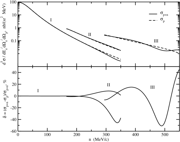
Figure 4: The electrodisintegration cross section versus the neutron momentum for three kinematics of the experiments at Saclay. Solid and dashed lines correspond to the calculations with and without neutron contribution (upper plot). Bottom plot shows the relative neutron contribution in the corresponding experimental regions. The experimental data regions were taken from [7]($Saclay_{I,II}$) and [8]($Saclay_{III}$).

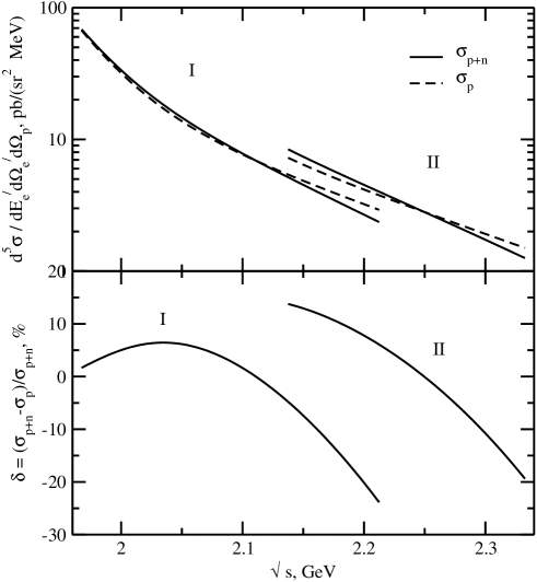
Figure 5: The same as in previous figure but versus pair invariant mass $\sqrt{s}$ for the kinematical conditions were taken from [9] ($Bonn_{I,II}$).

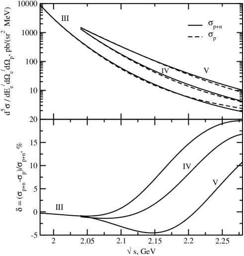
Figure 6: The same as in previous figure. The kinematical conditions were taken from [12]($Bonn_{III,IV,V}$).

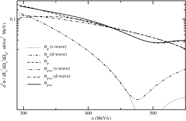
Figure 7: The contributions of the spectator neutron versus the outgoing neutron momentum to the electrodisintegration cross section of the deuteron partial $S$-, $D$-states are shown for the experimental sets from [8]($Saclay_{III}$).

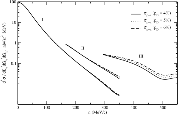
Figure 8: The contributions of the deuteron partial D-state to the electrodisintegration cross section versus neutron momenta are shown for three sets of the experiments [7]($Saclay_{I,II}$), [8] ($Saclay_{III}$).

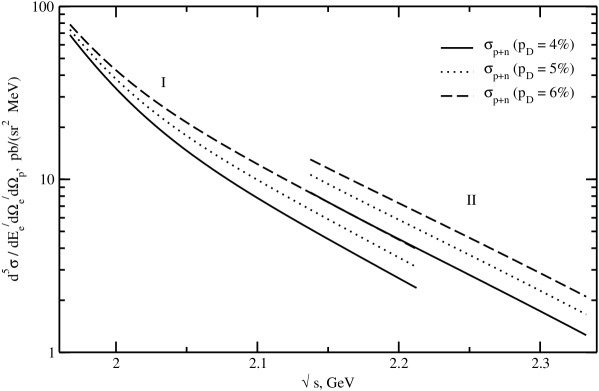
Figure 9: The contributions of the deuteron partial D-state to the electrodisintegration cross section versus pair invariant mass $\sqrt{s}$ are shown for the conditions of the experiments [9] ($Bonn_{I,II}$).

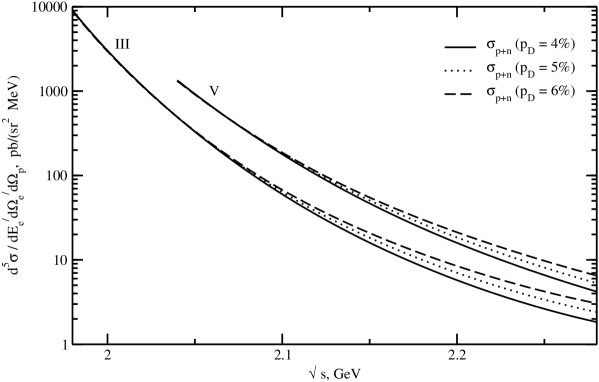
Figure 10: The same as in the previous figure but for [12] conditions ($Bonn_{III,V}$). We omitted curves for the $Bonn_{IV}$ case because they are very close to $Bonn_{V}$.

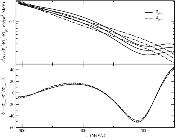
Figure 11: The contribution of the spectator neutron versus neutron momenta to the electrodisintegration cross section for different deuteron $D$-states for conditions of the experiment $Saclay_{III}$ [8]. In the first picture solid (dashed) line stands for $p+n$- ($p$-) contribution with different $D$-states in the deuteron: $p_{D}$ = 4% for lower line and $p_{D}$ = 6% for upper line.

7.  Summary

In the presented paper we have considered the electrodisintegration of the deuteron in the Bethe-Salpeter approach. It is realized for the two-nucleon system by using the multipole expansion with the spinor structure of two nucleons. The separable ansatz for the interaction kernel has provided a manageable system of linear homogeneous equations for deriving the BS amplitude.

We have switched then to the case with the use of the covariant revision of the Graz II separable potential with the summation of several separable functions.

The reaction of the deuteron electrodisintegration served as a testing ground for the method under investigation and helped to outline both strong and weak points of the approach. The analysis has proved the technique to be very promising, even if we find an evident discrepancies with experimental data at this stage of development. Several items can be suggested for the program of further theoretical study. First of all it is necessary to take into account the final state interaction for the $np$-pair. Then we need to take into account the negative-energy states for the BS amplitude and calculate the contribution of the $P$ waves in the electrodisintegration. After that we can calculate different asymmetries of the $(ed\to enp)$ process which can give new qualitative information about the structure of the deuteron.

Acknowledgments

We wish to thank our collaborators K.Yu. Kazakov, A.V. Shebeko, S.Eh. Shirmovsky, D.V. Shulga for their contribution to the presented work. We would like to thank Professor H.Toki and Professor D. Blaschke for their interest to this work and fruitful discussions.

The work is supported in part by the Russian Foundation for Basic Research, grant No.05-02-17698a.

References

[1] T. Wilbois, G. Beck, H. Arenhovel, Few-Body Syst., 15, p.39, 1993.
[2] G. Beck, T. Wilbois, H. Arenhovel, Few-Body Syst., 17, p.91, 1994.
[3] W.W. Buck, F. Gross, Phys. Rev., D20, p.2361, 1979.
[4] V. Dmitrasinovic, F. Gross, Phys. Rev., C40 p.2479, 1989.