Cold Uniform Matter and Neutron Stars in the Quark-Meson-Coupling Model

Abstract

A new density dependent effective baryon-baryon interaction has been recently derived from the quark-meson-coupling (QMC) model, offering impressive results in application to finite nuclei and dense baryon matter. This self-consistent, relativistic quark-level approach is used to construct the Equation of State (EoS) and to calculate key properties of high density matter and cold, slowly rotating neutron stars. The results include predictions for the maximum mass of neutron star models, together with the corresponding radius and central density, as well the properties of neutron stars with mass of order 1.4 $M_{\odot}$. The cooling mechanism allowed by the QMC EoS is explored and the parameters relevant to slow rotation, namely the moment of inertia and the period of rotation investigated. The results of the calculation, which are found to be in good agreement with available observational data, are compared with the predictions of more traditional EoS, based on the A18+$\delta$v+UIX^∗ and modified Reid soft core potentials, the Skyrme SkM^∗ interaction and a relativistic mean field (RMF) models for a hybrid stars including quark matter. The QMC EoS provides cold neutron star models with maximum mass 1.9–2.1 M_⊙, with central density less than 6 times nuclear saturation density ($n_{0}=0.16{\rm\ fm}^{-3}$) and offers a consistent description of the stellar mass up to this density limit. In contrast with other models, QMC predicts no hyperon contribution at densities lower than $3n_{0}$, for matter in $\beta$-equilibrium. At higher densities, $\Xi^{-,0}$ and $\Lambda$ hyperons are present. The absence of lighter $\Sigma^{\pm,0}$ hyperons is understood as a consequence of antisymmetrisation, together with the implementation of the color hyperfine interaction in the response of the quark bag to the nuclear scalar field.

1 Introduction

Nuclear forces play an important role in many stellar environments, acting in concert with gravitational forces to form compact objects. For example, the observed maximum mass of cold neutron stars cannot be explained without considering the pressure, arising from the strong nuclear force, which opposes gravitational collapse. It follows that strongly interacting matter is one of the fundamental systems that we have to study in order to understand stellar phenomena as well as the properties of finite nuclei.

The properties of stellar matter are strongly density dependent. The theoretical framework for describing the properties of strongly interacting matter is the Equation of State (EoS), which relates the pressure and total energy density of the system. These quantities are derived from the density dependence of the energy per particle of the system, calculated using a model for the baryon-baryon interaction between particles present in the matter. There is a large variety of EoS available in the literature (see e.g. [1, 2, 3, 4]), based on very different assumptions concerning the nature of the interactions governing the stellar matter. Ways of constraining the available EoS are being actively sought (see e.g. [4, 5, 6, 7, 8]) but no unambiguous findings have been reported as yet. The study of the properties of high density matter and of cold neutron stars provides an attractive laboratory for seeking such a constraint. However, the fundamental question arises as to the limit of applicability of any of the existing EoS at densities as high as $6\div 10\,n_{0}$, required, for example, for calculating the maximum mass of neutron star models.

At sufficiently high density, nuclear matter will most likely be composed not just of nucleons and leptons but also strange baryons and boson condensates [9, 10, 11, 12]. More importantly, it is unlikely that these particles will maintain their identity as confined entities of quarks, but the interaction between overlapping quark bags will result in partial or full deconfinement [13, 14]. Therefore a realistic high density EoS should contain all this physics. Numerical extrapolation of a nucleon-only EoS to high densities, although it may appear to work (mechanically), is dangerous and may obscure some important effects. This is true even at lower densities, in the region around twice nuclear saturation density, as some models predict low threshold densities for the creation of hyperons in beta equilibrium. The investigation of this effect on non-equilibrium matter is expected to be crucial for modelling core-collapse supernovae, as the density at bounce after the original collapse is around $2\div 2.5\,n_{0}$ and the presence of hyperons will soften the EoS, thus assisting the explosion.

The relativistic formulation of the QMC model [15, 16] offers a unique opportunity to self-consistently probe the composition of high density matter. In this work, the matter which is investigated is taken to be in $\beta$-equilibrium, including the full baryon octet as well as electrons and muons. The density and temperature dependent thresholds and production rates of hyperons in non-equilibrium stellar matter, relevant for core-collapse supernova physics, will be the subject of a forthcoming publication.

The general QMC model is briefly described in Section 2, followed by a description of its application to uniform nuclear matter at zero temperature and in $\beta$-equilibrium (Section 3). The basic features of cold, slowly rotating neutron stars are given in Section 4. Details of QMC neutron star models and some comparison with observational data and other model calculations are given in Section 5, with a summary of our main conclusions in Section 6.

2 QMC model

2.1 The physics of the model

The formulation of the QMC model [17] which we use in this work has been presented in a previous paper [16]. There it was shown that it is possible to build a nuclear Hamiltonian which is consistent with relativity and which can be used at high density. The predictions of this model, which represents a significant improvement over earlier work [15], because the need to expand about $<\sigma>=0$ was removed, have been sucessfully confronted with the phenomenology of finite nuclei. In this section we rely on the results of Ref. [16] and generalize the formalism to nuclear matter containing an arbitrary mixture of the octet members, $N,\Lambda,\Sigma,\Xi$.

We recall that, in the QMC model, the nuclear system is represented as a collection of quark bags. These bags may contain strange as well as non strange quarks, so the framework is well adapted to describing any kind of baryon. The crucial hypothesis is that in nuclear matter the baryons retain their individuality, or more precisely, they remain the pertinent degrees of freedom (or quasi-particles) even in dense nuclear matter. From this point of view the usual statement that the bags should not overlap is clearly too restrictive. It gives too much weight to the description of the internal structure within the bag model, while the latter is in fact used only to infer the interactions between the quasi-particles. In this respect, we point out that the bag model is an effective realisation of confinement, which must not be taken too literally. The QCD lattice simulations of Bissey et al. [18] indicate that the true confinement picture is closer to a Y-shaped color string attached to the quarks. Outside this relatively thin string one has the ordinary, non-perturbative vacuum, where the quarks from other hadrons can pass without disturbing the structure very much. So, even though the bag model imposes a strict condition, which prevents the quarks from travelling through its boundary, this must be seen as the average representation of a more complex situation and one should not attribute a deep physical meaning to the surface of the cavity nor to its size. In particular, estimating the density at which the QMC approximation breaks down as the reciprocal of the bag volume is certainly too pessimistic. Of course, there is a density above which the QMC model becomes inadequate but in this work we assume that this critical density is large enough that we can use the model to predict the properties of neutron stars.

The salient feature of the QMC model is that the interactions are generated by the exchange of mesons coupled locally to the quarks. In a literal interpretation of the bag model, where only quarks and gluons can live inside the cavity, this coupling would be unnatural. Again, we must return to the more realistic underlying picture where the quarks are attached to a string but otherwise move in the non-perturbative QCD vacuum. There, nothing prevents them from feeling the vacuum fluctuations, which we describe by meson fields. As before we limit our considerations to the $\sigma,\,\omega$ and $\rho$ mesons. We also estimate, in a simplified manner, the effect of single pion exchange. At this point it is useful to recall that the $\sigma$ meson used here is not the chiral partner of the pion. It is a chiral invariant scalar field, which mocks up the correlated multi-pion exchanges in the scalar-isoscalar channel.

2.2 Effective mass and energy of a bag in the nuclear medium

In Ref. [19] we used the Born-Oppenheimer (BO) approximation to derive the energy of a quark bag coupled to the nuclear mean fields associated with the $\sigma,\,\omega$ and $\rho$ mesons. Given the position and velocity of a bag, we obtained its energy by solving the field equations for the confined quarks. As the BO approximation requires that both position and velocity are known, this energy is of course classical and canonical quantization is performed after the full Hamiltonian has been built. As our previous work was limited to nuclear matter and finite nuclei built primarily of nucleons, we now generalize our results to include hyperons. Here we limit our considerations to the spin 1/2 SU(3) octet $(N,\Lambda,\Sigma,\Xi)$ and therefore a baryon can be specified by $|f>=|tms>$, with $t,m$ the isospin and its projection and $s$ the strangeness – see Table 1.

	$p$	$n$	$\Lambda$	$\Sigma^{-}$	$\Sigma^{0}$	$\Sigma^{+}$	$\Xi^{-}$	$\Xi^{0}$
$t$	$\frac{1}{2}$	$\frac{1}{2}$	0	1	1	1	$\frac{1}{2}$	$\frac{1}{2}$
$m$	$\frac{1}{2}$	$-\frac{1}{2}$	0	-1	0	1	$-\frac{1}{2}$	$\frac{1}{2}$
$s$	0	0	-1	-1	-1	-1	-2	-2

Table 1: Quantum numbers of the octet members.

Our working hypothesis is that the strange quark is not coupled to the meson fields, which can be seen as a consequence of the fact that the mesons represent correlated pion exchanges. This is also the natural explanation for the small spin-orbit splitting observed in $\Lambda$ hypernuclei, given that all the $\Lambda$ spin is carried by the strange quark. We set the $u$ and $d$ quark masses to zero and assume that their coupling to the meson fields respects isospin symmetry. Then the energy of a baryon of flavour $f$ with position $\vec{R}$ and momentum $\vec{P}$ has the form

$$E=\sqrt{P^{2}+M_{f}(\sigma)^{2}}+g_{\omega}^{f}\omega+g_{\rho}\vec{b}.\vec{I}^{t}$$ (1)

where $M_{f}(\sigma)$ is the effective mass, that is the energy of the corresponding quark bag in its rest frame, in the $\sigma$ field, and $\vec{I}^{t}$ is the isospin operator for isospin $t$, defined as

$$<tms|\sum_{q}\frac{\vec{\tau_{q}}}{2}|t^{\prime}m^{\prime}s^{\prime}>=\delta(tt^{\prime})\delta(ss^{\prime})\vec{I}_{mm^{\prime}}^{t}$$ (2)

with $\vec{\tau}_{q}$ the Pauli matrix acting on the $u$ and $d$ quarks. Apart from the $\rho$ coupling, for which we denote the field $b_{\alpha}$, with $\alpha=(-1,0,1)$ the isospin index, the energy is diagonal in flavour space. Note that the flavour dependence of the $\rho$ coupling is entirely contained in $\vec{I}^{t}$. In Eq. (1) the meson fields are evaluated at $\vec{r}=\vec{R}$, the center of the bag and, in comparison with Ref. [16], we have dropped the spin-orbit interaction – since in the following we shall consider only the case of uniform matter. The flavour dependence of the $\omega$ coupling is fixed by the number of non-strange quarks in the baryon, that is:

$$g_{\omega}^{f}=w_{f}^{\omega}g_{\omega}=(1+\frac{s}{3})g_{\omega}$$ (3)

with $g_{\omega}$ the $\omega-N$ coupling constant. As shown in the Appendix, the effective mass is well approximated by a quadratic expansion

$$M_{f}(\sigma)=M_{f}-w_{f}^{\sigma}g_{\sigma}\sigma+\frac{d}{2}\tilde{w}_{f}^{\sigma}\left(g_{\sigma}\sigma\right)^{2}$$ (4)

where $g_{\sigma}$ is the free $\sigma-N$ coupling constant. The scalar polarisability, $d$, describes the response of the nucleon to the applied scalar field. It is at the origin of the many-body forces in the QMC model. The corresponding scalar polarisability for baryon $f$ is $d\tilde{w}_{f}^{\sigma}(w_{f}^{\sigma})^{-2}$. The weights $w_{f}^{\sigma},\tilde{w}_{f}^{\sigma}$ control the flavour dependence and in first approximation $w_{f}^{\sigma}\simeq\tilde{w}_{f}^{\sigma}\simeq 1+s/3.$ The hyperfine color interaction breaks this relation and the exact values, which depend on the free nucleon radius, $R_{N}^{free}$, are given in the Appendix.

2.3 Hamiltonian

The total energy of the nuclear system is the sum of the baryon energies (1) and of the energy stored in the meson fields:

$$E_{tot} = \sum_{i=1,A}E(i)+E_{mesons}$$

$$E_{mesons} = \frac{1}{2}\int d\vec{r}\left[\left(\nabla\sigma\right)^{2}+m_{\sigma}^{2}\sigma^{2}\right]$$ (5)

$$-\frac{1}{2}\int d\vec{r}\left[\left(\nabla\omega\right)^{2}+m_{\omega}^{2}\omega^{2}\right]-\frac{1}{2}\int d\vec{r}\left[\left(\nabla\vec{b}\right)^{2}+m_{\rho}^{2}\vec{b}^{2}\right]$$

with $m_{\sigma},m_{\omega},m_{\rho}$ the meson masses. As usual, we consider only the time component of the vector fields. By hypothesis, the meson fields are time independent. Therefore the classical Hamiltonian of the nuclear system is simply

$$H(R_{i},P_{i})=E_{tot}(R_{i},P_{i},\sigma\to\sigma_{sol},\omega\to\omega_{sol},\vec{b}\to\vec{b}_{sol})$$ (6)

where $\sigma_{sol},\omega_{sol},\vec{b}_{sol}$ are the the solutions of the meson equations of motion:

$$\frac{\delta E}{\delta\sigma}=\frac{\delta E}{\delta\omega}=\frac{\delta E}{\delta b_{\alpha}}=0.$$ (7)

The equations for the $\omega,\vec{b}$ fields, which are linear, present no difficulty. By contrast, the $\sigma$ field equation is highly non-linear, because of the scalar polarisability term in the effective mass. In Ref. [16], we proposed to solve it approximately by writing:

$$\sigma=\bar{\sigma}+\delta\sigma,\ \ \ \bar{\sigma}=<\sigma>$$ (8)

where, $<\cdots>$, denotes the nuclear ground state expectation value, and we considered the deviation, $\delta\sigma$, as a small quantity. We refer to Ref. [16] for the details of the derivation and here we simply recall the results. The piece of the Hamiltonian which depends on $\sigma$ may be written:

$$H_{\sigma}=\int d\vec{r}\,\left[K(\bar{\sigma})-\frac{1}{2}\bar{\sigma}<\frac{\partial K}{\partial\bar{\sigma}}>+\frac{1}{2}\delta\sigma\left(\frac{\partial K}{\partial\bar{\sigma}}-<\frac{\partial K}{\partial\bar{\sigma}}>\right)\right]$$ (9)

where normal ordering is implicit. The one body kinetic energy operator, $K(\bar{\sigma})$, is defined as ($V$ is the normalization volume):

$$K(\bar{\sigma})=\frac{1}{2V}\sum_{\vec{k},\vec{k}^{\prime},f}e^{i(\vec{k}-\vec{k}^{\prime}).\vec{r}}\left(\sqrt{k^{2}+M_{f}[\bar{\sigma}(\vec{r})]^{2}}+\sqrt{k^{\prime 2}+M_{f}[\bar{\sigma}(\vec{r})]^{2}}\right)a_{\vec{k}f}^{\dagger}a_{\vec{k}^{\prime}f}$$ (10)

with $a_{\vec{k}f}$ the destruction operator for a baryon of momentum $\vec{k}$ and flavour $f$, the spin label being omitted for simplicity. Note that the mean field approximation amounts to setting $\delta\sigma=0$ in the Hamiltonian (9).

The meson field solution in the general case is of little interest to us, so we directly give the solution for a uniform system in which case $\bar{\sigma}$ is a constant determined by the self consistent equation:

$$\bar{\sigma}=-\frac{1}{m_{\sigma}^{2}}<\frac{\partial K}{\partial\bar{\sigma}}>$$ (11)

which must be solved numerically and the fluctuation $\delta\sigma$ is given by:

$$\delta\sigma(\vec{r})=\int d\vec{r}^{\prime}\frac{d\vec{q}}{(2\pi)^{3}}\frac{e^{i\vec{q}.(\vec{r}-\vec{r}^{\prime})}}{q^{2}+\tilde{m}_{\sigma}^{2}}\left(-\frac{\partial K}{\partial\bar{\sigma}}(\vec{r}^{\prime})+<\frac{\partial K}{\partial\bar{\sigma}}>\right)$$ (12)

where the effective $\sigma$ mass is:

$$\tilde{m}_{\sigma}^{2}=m_{\sigma}^{2}+<\frac{\partial^{2}K}{\partial\bar{\sigma}^{2}}>.$$ (13)

2.4 Energy density in the Hartree Fock approximation

The last step in our formal development is to use Eqs. (9-12) to compute the energy density of nuclear matter in the Hartree-Fock approximation. The ground state of the system is specified by a set of Fermi levels, $\{k_{F}(f),f=p,n...\}$, and their corresponding baryonic densities $\{n_{f}\}$ with $n_{B}=\sum_{f}n_{f}$. One has:

$$<K(\bar{\sigma})>=\frac{2}{(2\pi)^{3}}\sum_{f}\int_{o}^{k_{F}(f)}d\vec{k}\sqrt{k^{2}+M_{f}^{2}(\bar{\sigma})}$$ (14)

and the energy density takes the form

$$\frac{<H_{\sigma}>}{V} = <K(\bar{\sigma})>+\frac{1}{2m_{\sigma}^{2}}\left(<\frac{\partial K}{\partial\bar{\sigma}}>\right)^{2}+\frac{1}{(2\pi)^{6}}\sum_{f}\int_{0}^{k_{F}(f)}d\vec{k}_{1}d\vec{k}_{2}$$ (15)

$$\frac{1}{(\vec{k}_{1}-\vec{k}_{2})^{2}+\tilde{m}_{\sigma}^{2}}\frac{\partial}{\partial\bar{\sigma}}\sqrt{k_{1}^{2}+M^{2}(\bar{\sigma})}\frac{\partial}{\partial\bar{\sigma}}\sqrt{k_{2}^{2}+M^{2}(\bar{\sigma})}.$$

Finally we must add the contributions $<V_{\omega}>and<V_{\rho}>$, corresponding to $\omega$ and $\rho$ exchange. The derivation follows the same line as for the $\sigma$ exchange but is much simpler and gives the exact solution because these interactions are purely 2-body . One gets:

$$\frac{<V_{\omega}>}{V}=\frac{G_{\omega}}{2}\left(\sum_{f}w_{f}^{\omega}n_{f}\right)^{2}$$

$$-G_{\omega}\sum_{f}\left(w_{f}^{\omega}\right)^{2}\frac{1}{(2\pi)^{6}}\int_{0}^{k_{F}(f)}d\vec{k}_{1}d\vec{k}_{2}\frac{m_{\omega}^{2}}{(\vec{k}_{1}-\vec{k}_{2})^{2}+m_{\omega}^{2}}$$ (16)

$$\frac{<V_{\rho}>}{V}=\frac{G_{\rho}}{2}\left(\sum_{tms}mn_{tms}\right)^{2}$$

$$-G_{\rho}\sum_{tmm^{\prime}s}\vec{I}_{mm^{\prime}}^{t}.\vec{I}_{m^{\prime}m}^{t}\frac{1}{(2\pi)^{6}}\int_{0}^{k_{F}(tms)}d\vec{k}_{1}\int_{0}^{k_{F}(tm^{\prime}s)}d\vec{k}_{2}\frac{m_{\rho}^{2}}{(\vec{k}_{1}-\vec{k}_{2})^{2}+m_{\rho}^{2}}$$ (17)

As usual we define:

$$G_{\sigma}=\frac{g_{\sigma}^{2}}{m_{\sigma}^{2}},\,G_{\omega}=\frac{g_{\omega}^{2}}{m_{\omega}^{2}},\,G_{\rho}=\frac{g_{\rho}^{2}}{m_{\rho}^{2}}.$$ (18)

The $\sigma,\omega$ and $\rho$ mesons represent the multi-pion exchanges that we believe to be the most relevant ones. However, this cannot take into account the long ranged single pion exchange. In the Hartree Fock approximation, the latter contributes only through the exchange (Fock) term, so its contribution to the energy is modest. Nevertheless, we think it is worthwhile to study its impact on our results because, as a consequence of its long range, the pion contribution to the energy has, as compared to the heavy mesons, a specific density dependence. With this in mind, we generalize the expression of Ref. [20] so as to include the contribution of the full octet. We get:

$$\frac{<V_{\pi}>}{V} = \frac{1}{n_{B}}\left(\frac{g_{A}}{2f_{\pi}}\right)^{2}\left\{J_{pp}+4J_{pn}+J_{nn}-\frac{24}{25}\left(J_{\Lambda,\Sigma^{-}}+J_{\Lambda,\Sigma^{0}}+J_{\Lambda,\Sigma^{+}}\right)\right.$$ (19)

$$+ \left.\frac{16}{25}\left(J_{\Sigma^{-}\Sigma^{-}}+2J_{\Sigma^{-}\Sigma^{0}}+2J_{\Sigma^{+}\Sigma^{0}}+J_{\Sigma^{+}\Sigma^{+}}\right)\right.$$

$$+ \left.\frac{1}{25}\left(J_{\Xi^{-}\Xi^{-}}+4J_{\Xi^{-}\Xi^{0}}+J_{\Xi^{0}\Xi^{0}}\right)\right\}$$

with :

$$J_{ff^{\prime}} = \frac{1}{(2\pi)^{6}}\int^{k_{F}(f)}\int^{k_{F}(f^{\prime})}d\vec{p}d\vec{p}^{\prime}\left[1-\frac{m_{\pi}^{2}}{(\vec{p}-\vec{p}^{\prime})^{2}+m_{\pi}^{2}}\right].$$ (20)

In Eq. (19), $g_{A}=1.26$ is the axial coupling constant of the nucleon, $f_{\pi}=93{\rm\ MeV}$ is the pion decay constant and $m_{\pi}$ its mass. In the loop integral $J_{ff^{\prime}}$, the first term is the so-called contact term. In practice it can hardly be distinguished from the short-ranged contributions of the heavy mesons and we omit it. We have checked that it would only induce a small readjustment of $G_{\sigma},G_{\omega},G_{\rho}$. In the same spirit we have omitted any $\pi$-baryon form factor in $J_{ff^{\prime}}$, because the effect of a form factor is to cut off the large momenta of the loop and it therefore amounts to a short ranged contribution. In summary, we keep only the long ranged Yukawa piece of the pion exchange.

2.5 Fixing the parameters

The parameters of the model are the couplings $G_{\sigma},G_{\omega},G_{\rho}$, the meson masses and the free nucleon radius. We set the $\pi,\omega,\rho$ masses to their physical values. We have tried several values of the free nucleon radius, $R_{N}^{free}$, and found that this has very little influence on our results. We therefore take $R_{N}^{free}=0.8{\rm\ fm}$, which is a realistic value [21]. The $\sigma$ meson mass is not well known because the width of the $\pi\pi$ resonance is very large in the physical region. In our study of finite nuclei [16], we found that $m_{\sigma}\sim 700{\rm\ MeV}$ produced the best results, so this will be our prefered value. However, the sensitivity of the calculations of finite nuclei to the $\sigma$ meson mass comes from the fact that it controls the shape of the nuclear surface, a factor which is irrelevant in the case of neutron stars. Moreover, since the calculations for finite nuclei are based on a non-relativistic, low density approximation to the Hamiltonian (9), we must be conservative about the $\sigma$ meson mass when we use it in the high density region. Therefore, to quantify the influence of this mass, we shall show some results for $m_{\sigma}=600{\rm\ MeV}.$

The remaining free parameters, $G_{\sigma},G_{\omega}$ and $G_{\rho}$ are adjusted to reproduce the binding energy and the asymmetry energy of ordinary nuclear matter at the saturation point. Since we want to sample the stiffness of our equation of state, we allow some freedom in the way the couplings are fixed. This is summarized in Table 2. First we set the pion contribution to zero and adjust the couplings to reproduce the experimental values of the binding energy, $({\mathcal{E}}=-15.865{\rm\ MeV})$, and asymmetry energy, $(a_{s}=30{\rm\ MeV})$, of nuclear matter at the saturation point ($n_{0}=0.16{\rm\ fm}^{-3}$). This defines the models QMC600 and QMC700, according to the value of the $\sigma$ meson mass. For all the other models (QMC$\pi i,\,i=1,4$) we set $m_{\sigma}=700{\rm\ MeV}$ and the effect of the pion is included. As can be seen in the last column of Table 2, the incompressibility modulus of both QMC600 and QMC700 is above the accepted range, $200\div 300{\rm\ MeV}$. The most efficient way to decrease $K_{\infty}$ is to add an attractive interaction which has a weak density dependence at the saturation point. The pion Fock term, which is attractive and behaves roughly as $\rho^{1/6}$ , is thus a natural candidate. This is confirmed by the model QMC$\pi 1$, where the pion contribution is included and where $K_{\infty}$ drops from $340{\rm\ MeV}$ to $322{\rm\ MeV}$. A trivial way to mock up the effect of an almost constant attractive interaction is simply to decrease the absolute value of the experimental binding energy. By setting ${\mathcal{E}}=-14.5{\rm\ MeV}$, a rather moderate distortion of the experimental number, we already find $K_{\infty}=301{\rm\ MeV}.$ This defines QMC$\pi 2.$ In order to sample a wider range of values of the stiffness, we allow ourself to artificially vary both the pion contribution and the binding energy. This leads to model QMC$\pi 3$ (resp. QMC$\pi 4$), where the pion contribution is multiplied by 1.5 (resp. 2) and the binding energy is set to $-14{\rm\ MeV}$ (resp $-13{\rm\ MeV}$). This gives $K_{\infty}=283{\rm\ MeV}$ and $K_{\infty}=256{\rm\ MeV}$, respectively. Note that increasing the pion contribution by a factor of 2 is not so arbitrary, because we know that it is amplified by RPA correlations [22]. On the other hand, changing the experimental binding energy is more difficult to justify and we take it only as a crude way to sample the stiffness of the model, given its eventual application in the high density region, far away from the point where ${\mathcal{E}}$ is measured.

Model	$m_{\sigma}({\rm\ MeV})$	$\pi$	${\mathcal{E}}({\rm\ MeV})$	$G_{\sigma}({\rm\ fm}^{2})$	$G_{\omega}({\rm\ fm}^{2})$	$G_{\rho}({\rm\ fm}^{2})$	$K_{\infty}({\rm\ MeV})$
QMC600	600	0	-15.865	11.23	7.31	4.81	344
QMC700	700	0	-15.865	11.33	7.27	4.56	340
QMC$\pi 1$	700	1	-15.865	10.64	7.11	3.96	322
QMC$\pi 2$	700	1	-14.5	10.22	6.91	3.90	301
QMC$\pi 3$	700	1.5	-14	9.69	6.73	3.57	283
QMC$\pi 4$	700	2	-13	8.97	6.43	3.22	256

Table 2: The couplings for different versions of the model. The column $\pi$ is the number by which the pion contribution has been multiplied. ${\mathcal{E}}$ is the binding energy of symmetric nuclear matter and $K_{\infty}$ its incompressibility modulus.

3 Cold Uniform Matter

In this section we determine the equation of state of uniform matter, which is directly relevant for studies of the interior of neutron stars. The structure of the neutron stars is discussed in the next section. Uniform matter in cold neutron stars is in a generalized beta-equilibrium, achieved over an extended period of time. All baryons of the octet can be populated by succcessive weak interactions, regardless of their strangeness [23]. We consider matter formed by baryons of the octet, electrons and negative muons, with respective densities $\{n_{f},f=p,n,...\}$ and $\{n_{e},n_{\mu}\}.$

The equilibrium state minimises the total energy density, $\epsilon$, under the constraint of baryon number conservation and electric neutrality. We write:

$$\epsilon=\epsilon_{B}(n_{p},...)+\epsilon_{e}(n_{e})+\epsilon_{\mu}(n_{\mu})$$ (21)

where the baryonic contribution

$$\epsilon_{B}(n_{p},...)=\frac{<H_{\sigma}+V_{\omega}+V_{\rho}+V_{\pi}>}{V}$$ (22)

is calculated from Eqs. (15-19). It is related to the binding energy per baryon, ${\mathcal{E}}$, by:

$$\epsilon_{B}(n_{p},...)=\sum_{f}({\mathcal{E}}+M_{f})n_{f}.$$ (23)

The baryonic pressure, ($P_{B}$), the incompressibility modulus, ($K_{\infty}$), and the sound velocity, ($v_{s}$), of baryonic matter have the following expressions:

$$P_{B}=n_{B}^{2}\frac{\partial}{\partial n_{B}}\frac{\epsilon_{B}}{n_{B}},\,\,\,K_{\infty}=9\frac{\partial P_{B}}{\partial n_{B}},\,\,\,v_{s}=\sqrt{\frac{n_{B}K_{\infty}}{9(\epsilon_{B}+P_{B})}}$$ (24)

where $n_{B}=\sum_{f}n_{f}$ and the derivative, with respect to $n_{B}$, is taken at constant fractions $(n_{f}/n_{B},f=1,8)$. Similar expressions hold for each lepton. In proton-neutron matter another important variable is the symmetry energy, ${\mathcal{S}}$, defined as the difference between pure neutron and symmetric matter :

$${\mathcal{S}}(n_{B})={\mathcal{E}}(\left(n_{p}=0,\,n_{n}=n_{B}\right)-{\mathcal{E}}\left(n_{p}=n_{B}/2,\,n_{n}=n_{B}/2\right).$$ (25)

For the energy density of the lepton $l$, of mass $m_{l}$ and density $n_{l}$, we use the free Fermi gas expression:

$$\epsilon_{l}(n_{l})=\frac{2}{(2\pi)^{3}}\int^{k_{F}(l)}d\vec{k}\sqrt{k^{2}+m_{l}^{2}},\,\,\,{\rm with}\,n_{l}=\frac{k_{F}^{3}(l)}{3\pi^{2}}.$$ (26)

The equilibrium condition for a neutral system with baryon density $n_{B}$ is

$$\delta[\epsilon_{B}(n_{p},...)+\epsilon_{e}(n_{e})+\epsilon_{\mu}(n_{\mu})$$

$$+\lambda(\sum_{f}n_{f}-n_{B})+\nu(\sum_{f}n_{f}q_{f}-(n_{e}+n_{\mu})]=0$$ (27)

where $q_{f}$ is the charge of the flavor $f$. The constraints are implemented through the Lagrange multipliers $(\lambda,\nu)$ so the variation in Eq. (27) amounts to independent variations of the densities, together with variations of $\lambda$ and $\nu$. If one defines the chemical potentials as

$$\mu_{f}=\frac{\partial\epsilon_{B}}{\partial n_{f}},\,\,\,\mu_{l}=\frac{\partial\epsilon_{l}}{\partial n_{l}}=\sqrt{k_{F}^{2}(l)+m_{l}^{2}}$$ (28)

the equilibrium equations become:

$$\mu_{i}+\lambda+\nu q_{i} = 0,\,\,\,f=p,...,$$ (29)

$$\mu_{e}-\nu = 0,$$ (30)

$$\mu_{\mu}-\nu = 0,$$ (31)

$$\sum_{f}n_{f}-n_{B} = 0,$$ (32)

$$\sum_{f}n_{f}q_{f}-(n_{e}+n_{\mu}) = 0.$$ (33)

This is a system of non-linear equations for $\{n_{p},...,n_{e},n_{\mu},\lambda,\nu\}.$ It is usual to eliminate the Lagrange multipliers, $(\lambda,\nu)$, using Eqs. (30) and (29), with $f=neutron.$ However, for a given value of $n_{B}$, the equilibrium equation, Eq. (27), generally implies that some of the densities vanish and therefore that the equations generated by their variation drop from the system (29-31) – because there is nothing to vary! In particular, substituting $\nu=\mu_{e}$ in Eqs. (29) is not valid when the electron disappears from the system. The equations obtained by this substitution may have no solution in the deleptonized region, since one has forced $\nu=0$. To correct for this, one must restore $\nu$ as an independent variable when one reaches this region. This is technically inconvenient and we found it is much simpler to blindly solve the full system of equations, (29-33), for the set $\{n_{p},...,n_{e},n_{\mu},\lambda,\nu\}$. The only simplification which is not dangerous is the elimination of the muon density in favor of the electron density by combining Eqs. (30,31) to write $\mu_{\mu}=\mu_{e}$, which is solved by

$$k_{F}(\mu)=\Re\sqrt{k_{F}(e)^{2}+m_{e}^{2}-m_{\mu}^{2}}$$ (34)

where $\Re$ denotes the real part. This is always correct because if the electron density vanishes then so does the muon density and the relation (34) reduces to $0=0.$

To solve the system (29-33), let us define the set of relative concentrations (note that the lepton concentrations are also defined with respect to $n_{B}$)

$$Y=\{y_{i}\}=\left\{\frac{n_{p}}{n_{B}},\frac{n_{n}}{n_{B}},\frac{n_{\Lambda}}{n_{B}},...,\frac{n_{e}}{n_{B}},\frac{n_{\mu}}{n_{B}}\right\}.$$ (35)

Each member, $y_{i}$, of the set $Y$ is associated with an equation $E_{i}$ , the one among Eqs. (29,31) which is obtained by taking the variation of $\epsilon$ with respect to $\rho_{i}=y_{i}n_{B}$. Let us assume that a solution, $Y_{0}$, has been found at some baryon density, $n_{B}=n_{0}$. One first tests whether the threshold for some species, $i$, is crossed when $n_{0}$ is incremented by $\delta n$. Since $y_{i}=0$ below and across the theshold, the condition for the appearance of the species is that $E_{i}(n_{B},Y_{0})$ changes its sign between $n_{0}$ and $n_{0}+\delta n$. If this happens, the equation $E_{i}$ is added to the system. If the threshold condition is met for several species, all the corresponding equations are added. The system is then solved numerically at $n_{B}=n_{0}+\delta n_{0}$, using $Y_{0}$ as a first approximation. When a concentration drops below a given small number, $\eta$, it is set to zero and the corresponding equation is removed from the system. The value of $\eta$ depends on the accuracy of the solution and in our calculation it has been set to $10^{-4}$. We have checked that $\eta=10^{-3}$ gives the same result. We solve the system with the initial condition that at $n_{B}=0$ the matter contains only neutrons. Once the equilibrium solution $Y(n_{B})$ has been found for the desired range of baryon density, typically $n_{B}=0\div 1.2{\rm fm}^{-3}$, it is used to compute the equilibrium total energy density, $\epsilon(n_{B})=\epsilon(y_{p}n_{B},...,y_{\mu}n_{B})$. The corresponding total pressure, $P(n_{B})$, is computed as the sum of the baryon pressure, (24), and of the lepton pressures. Using the equilibrium equations, Eqs. (29-33), it is straightforward to show that the total pressure can also be evaluated as (note the total derivative):

$$P(n_{B})=n_{B}^{2}\frac{d}{dn_{B}}\frac{\epsilon(n_{B})}{n_{B}}.$$ (36)

As a numerical check, we used both expressions, which did indeed yield the same result within the numerical accuracy.

4 Neutron Stars

A neutron star is an object composed of matter at densities ranging from that of terrestrial iron up to several times that of nuclear matter. In cold neutron stars, as the baryon density $n_{\rm B}$ increases from about 0.75 $n_{\rm 0}$ up to $2\div 3n_{\rm 0}$, stellar matter becomes a homogeneous system of unbound neutrons, protons, electrons and muons and, if enough time is allowed, will develop $\beta$-equilibrium with respect to the weak interactions. All components that are present on a timescale longer than the life-time of the system take part in equilibrium. For example, neutrinos created in weak processes in a cold neutron star do not contribute to the equilibrium conditions as they escape rapidly. At even higher densities, heavier mesons and strange baryons play a role (see e.g. Ref. [24] and references therein, [25, 26, 27, 28]). Ultimately, at the center of the star, a quark matter phase may appear, either alone or coexisting with hadronic matter  [23, 29, 30, 31]. Below $n_{\rm B}$ $\sim$ 0.75 $n_{\rm 0}$, the matter forms the inner and outer crust of the star, with inhomogeneities consisting of nucleons arranged on a lattice, as well as neutron and electron gases. In this density region the QMC Equation of State (EoS) needs to be matched onto other equations of state, reflecting the composition of matter at those densities. The Baym-Bethe-Pethick (BBP) [32] and Baym-Pethick-Sutherland (BPS) EoS [33] are used in this work.

Setting up an EoS over the full density range, up to at least 6 $n_{\rm 0}$, allows calculation of one of the most important observables of neutron stars, the maximum gravitational mass, $M_{\rm g}^{\rm max}$, and the corresponding radius, $R_{\rm max}$. The most accurately measured masses of neutron stars were, until very recently, consistent with the range 1.26 to 1.45 M_⊙ [5]. However, Nice et al. [34] recently provided a dramatic result for the gravitational mass of the PSR J0751+1807 millisecond pulsar (in a binary system with a helium white dwarf), M_g = 2.1$\pm$ 0.2 M_⊙ (with 68% confidence) or 2.1${}^{\rm+0.4}_{\rm-0.5}$ with 95% confidence which makes it the most massive pulsar measured. This observation potentially offers one of the most stringent tests for the EoS used in the calculation of cold neutron stars. It also sets an upper limit to the mass density, or equivalently, the energy density, inside the star [5]. A lower limit to the mass density can be derived using the latest data on the largest observed redshift from a neutron star, combined with its observational gravitational mass.

The calculated maximum mass is determined to large extent by the high density EoS. It has been argued that extrapolation of the nucleon-based EOS, built using an effective force (e.g. non-relativistic Skyrme [4], relativistic mean field [23]) or phenomenological interactions (such as A18+$\delta v$+ UIX^∗ (APR) [35]) to densities corresponding to $M_{\rm g}^{\rm max}$, may not be unreasonable [35, 36] and that the error made by not including the heavy baryons and possible quarks in the calculation may not be significant. On the other hand, we note that in the hybrid calculations of Lawley et al. [13], the maximum mass of a neutron star was significantly reduced. In any case, we will explore the consequences of this extrapolation by using the QMC EoS and taking into account the different composition of the homogeneous matter, starting from a nucleon-only model and then including the full baryon octet. We shall also comment shortly on the presence of exotics, such as penta-quarks and 6-quarks bags, in high density matter. Furthermore, neutron star models at around the ‘canonical’ mass of $1.4M_{\odot}$, with central densities of the order $2\div 2.5\,n_{0}$ and lower, are also studied as representative cases for nucleon-only based EoS.

4.1 Cold non-rotational neutron star models

The gravitational mass and the radius are calculated using a tabulated form of the composite EoS with a chosen QMC interaction. The Tolman-Oppenheimer-Volkov equation [37, 38]

$$\frac{dP}{dr}=-\frac{Gm\rho}{r^{2}}\ \frac{\left(1+{P}/{\rho}\right)\left(1+{4\pi r^{3}P}/{m}\right)}{1-{2Gm}/{r}}$$ (37)

is integrated with

$$m(r)=\int_{0}^{r}4\pi{r^{\prime}}^{2}\rho(r^{\prime})\,dr^{\prime},$$ (38)

where $\rho$ is the total mass density and $G$ is the gravitational constant, in order to obtain sequences of neutron-star models corresponding to any specified central mass density. The solution gives directly the radius, $R$, of the star (the surface being at the location where the pressure vanishes) and the corresponding value for the total gravitational mass $M_{g}=m(R)$.

It is also important to calculate some other properties of these neutron star models. The total baryon number $A$ is given by

$$A=\int_{0}^{R}\frac{4\pi r^{2}n_{\rm B}(r)dr}{\left(1-{2Gm(r)}/{r}\right)^{1/2}}\quad.$$ (39)

The total baryon number, $A$, multiplied by the atomic mass unit, 931.50  MeV, defines the baryonic mass M₀. The binding energy released in a supernova core-collapse, forming eventually the neutron star, is approximately

$$E_{bind}=(Am_{\rm 0}-M_{\rm g})\quad,$$ (40)

where $m_{\rm 0}$ is defined as the mass per baryon of ⁵⁶Fe. Analysis of data from supernova 1987A leads to an estimate of $E_{\rm bind}=3.8\pm 1.2\times 10^{53}$ erg [39].

The gravitational red shift of the photons emitted radially outwards from a neutron star surface is given by

$$z_{surf}=\left(1-\frac{2GM_{\rm g}}{R}\right)^{-1/2}-1$$ (41)

It is an important quantity needed, for example, for obtaining the mass and radius of a neutron star separately [5]. Other quantities of interest for possible comparison with observational data are the minimum rotation period, $\tau_{min}$ [40], and the moment of inertia ${\mathcal{I}}$ (see Ref. [6] and references therein). The minimum period is given by the centrifugal balance condition for an equatorial fluid element (i.e., the condition for it to be moving on a circular geodesic). While determining this accurately requires using a numerical code for constructing general-relativistic models of rapidly rotating stars, quite good values can be obtained from results for non-rotating models using the empirical formula [41, 42]

$$\tau_{min}=0.820\,\left(\frac{M^{\rm max}_{\rm g}}{M_{\odot}}\right)^{-1/2}\left(\frac{R_{\rm max}}{10\,{\rm km}}\right)^{3/2}\ {\rm ms}\,.$$ (42)

The shortest period so far observed is 0.877 ms [40] but it is possible that this limit may be connected with the techniques used for measuring pulsar periods, rather than being a genuine physical limit.

The moment of inertia $\mathcal{I}$ is calculated in this work by assuming that the rotation is sufficiently slow that the general relativistic slow rotation approximation [43] gives a rather accurate description of the star and the surrounding space-time and using the expressions given in Ref. [44].

5 Results and discussion

5.1 Uniform matter

The properties of uniform matter and neutrons stars were calculated for 12 EoS designed to systematically investigate the dependence on the basic QMC model parameters, summarised in Table 2. There are three types of EoS used in this work. They have the same QMC parameters but differ by the limitation that we impose on the matter composition. The sets F-QMCx, where x refers to the parametrisations of Table 2, describe matter consisting of the full baryon octet plus electrons and muons. The sets N-QMCx are used for $n+p+e+\mu$ matter and PNM-QMCx for pure neutron matter. For simplicity, we only show results for QMC700 and QMC$\pi 4$ in this section. These sets have the most realistic values of the QMC parameters and correspond to two rather different values of $K_{\infty}$, 340 and 256  MeV. In the next section all the QMC parametrisations of Table 2 are used for the calculation of neutron star models and their properties are discussed in more detail.

In addition to the QMC EoS, we use four other models for a comparison based on very different physics. The older Bethe-Johnson (BJ) EoS [45] is based on the modified Reid potential and the medium effects are treated using constrained variational principle (model C in [24]). The BJ EoS describes uniform matter including $n,p,\Lambda,\Sigma^{\rm\pm,0},\Delta^{\rm\pm,0}$ and $\Delta^{\rm++}$. The more recent EoS, calculated with the A18+$\delta v$+UIX^∗ potential (APR) [35], is based on the Argonne A18 two-body interaction and includes three-body effects through the Urbana UIX^∗ potential. It also includes boost corrections to the two-nucleon interaction which corresponds to the leading relativistic effects at order $v^{2}$. This interaction is considered one of the most modern phenomenological potentials used for the description of nuclear matter containing nucleons only. As an example of a phenomenological, nucleon-only EoS the Skyrme SkM^∗ interaction is used, in particular because of the similarity of its results for finite nuclei to those of the effective force derived from the QMC model [15, 16]. Finally, we also compare with the EoS of a hybrid (neutron-quark) star matter of Glendenning (Table 9.1 of [23]) (Hybrid) calculated in RMF approximation.

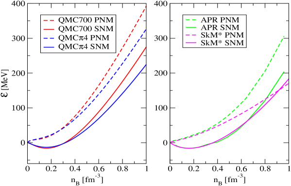
Figure 1: The energy per particle for pure neutron and symmetric nuclear matter is plotted as a function of baryon number density $n_{B}$ for the QMC700 and QMC$\pi 4$ interactions (left panel). For comparison, also shown are equivalent curves calculated using the APR potential [35] and the Skyrme SkM^∗ parametrisations (right panel)

The binding energy per particle in pure neutron matter (PNM) and symmetric nuclear matter (SNM), for QMC700 and QMC$\pi 4$, are illustrated in Fig. 1 in comparison with the APR and SkM^∗ predictions. At lower densities the calculated values are very similar. However, with increasing density the differences become more dramatic. In particular, while the QMC and APR models predict a steady increase of the energy per particle in both pure neutron and symmetric matter at about the same rate, the SkM^∗ model yields a more rapid growth of the energy per particle in SNM than in PNM, leading to crossing at about 0.9 fm^-3. As shown in Fig. 2 and discussed in detail in [4], this leads to negative symmetry energy and a collapse of nuclear matter. Although the QMC and Skyrme energy functionals have similar structure and yield similar results for finite nuclei at normal nuclear density, QMC has a different density and isospin dependence [16] that improves the EoS at high densities in comparison with SkM^∗, while the symmetry energy shows a slower increase with density than the APR model. There is no experimental evidence concerning the density dependence of the symmetry energy, as it is not possible to study the properties of uniform matter at high densities in terrestrial conditions. Even in heavy-ion collisions at high energies the maximum baryon density reached is unlikely to exceed $2\div 3n_{0}$ in the phase of the reaction closest to the conditions in cold neutron stars. Nevertheless, there is some indirect evidence which seems to support models which predict that the symmetry energy grows with density [4]. Such models yield sensible results for properties of neutron stars that can be compared with observations (see Section 4).

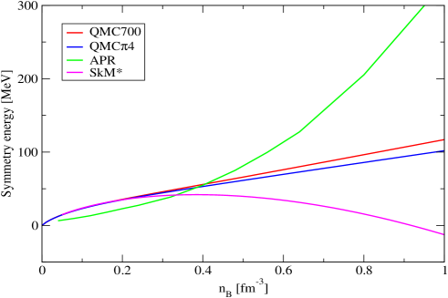
Figure 2: Symmetry energy as a function of baryon number density $n_{B}$ for QMC700 and QMC$\pi 4$. Also shown are the corresponding results for the APR potential and the Skyrme SkM^∗ parametrisations.

The results of our calculation of the equilibrium composition of uniform matter for QMC700 and QMC$\pi 4$ are shown in Fig. 3. In a striking difference from all other models which include the full baryon octet, QMC does not predict the production of hyperons at densities less than 3 times nuclear saturation density. Furthermore, the first hyperons to appear are the cascades, $\Xi$, together with the $\Lambda$ hyperon. The $\Sigma$ hyperons are not produced at densities below 1.2  fm^-3.

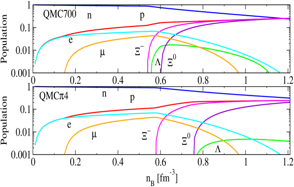
Figure 3: Relative population of baryons and leptons in $\beta$-equilibrium matter for QMC700 and QMC$\pi 4$. For more explanation see text.

This scenario is a direct consequence of three factors which are present in the QMC model and absent in the others. First, we use the Hartree-Fock approximation, while the earlier calculations worked only at the Hartree level. Actually, we see no reason to ignore antisymmetrisation, which is the key to our successful interpretation ofthe spectra of finite nuclei [16]. Second, the color hyperfine interaction, which is necessary to explain the mass splitting within the octet, as well as the $N\Delta$ splitting, induces a flavor dependent effective mass which strongly disfavors the $\Sigma$. Third, the scalar polarisability, $d$, induces many body effects which tend to amplify the previous ones.

To make these considerations quantitative, we have computed the single particle threshold densities on top of neutron matter, using the QMC700 parametrization and the variations on it defined earlier. The results are shown in Table 3, where the first column corresponds to the full QMC700 model as shown in Fig. 3. In the second column we show the same calculation but with the hyperfine color interaction and the scalar polarisability set to zero for the strange particles. Clearly this produces a very spectacular effect on the $\Sigma$ thresholds, which become comparable to the $\Xi$ thresholds. In the third column we show the same calculation as in the first but now in the Hartree approximation, that is dropping the exchange terms in Eqs. (15-17) and readjusting the coupling to reproduce the saturation point of nuclear matter. One observes again a strong rearrangement of the threshholds in favor of the $\Sigma$. Finally, the last column shows the combination of both effects. With these three alterations, the QMC model obviously becomes similar to the SU(3) relativistic mean field models – with respect to strangeness production. In particular, the first threshold is now for the $\Sigma^{-}$, almost identical to that for the $\Lambda$ and it occurs at less than twice the nuclear density.

	Hartree-Fock	Hartree-Fock	Hartree	Hartree
	QMC700	QMC700, hfc=d=0	QMC700	QMC700, hfc=d=0
$\Lambda$	0.555	0.42	0.35	0.31
$\Sigma^{-}$	0.92	0.51	0.41	0.3
$\Sigma^{0}$	0.97	0.58	0.61	0.44
$\Sigma^{+}$	1.01	0.63	0.87	0.61
$\Xi^{0}$	0.59	0.54	0.58	0.55
$\Xi^{-}$	0.55	0.50	0.45	0.43

Table 3: Single particle threshold densities (in fm^-3) on top of neutron matter for QMC700, either in Hartree or Hartree-Fock approximation and with the hyperfine color interaction (hfc) and scalar polarisability, $d$, set to zero in the strange sector.

As expected, the presence of hyperons does soften the EoS, as demonstrated in Fig. 4. We observe that QMC700 and QMC$\pi 4$ both show a very similar EoS to that for the BJ model, which also contains hyperons. However, it is clearly demonstrated that the composition of the stellar matter is not the only way to soften the EoS. The pressure also depends critically on the potentials acting between the particles present and, in turn, on the density dependence of the symmetry energy. Thus, for example, the SkM^∗ Skyrme model produces a very soft EoS, in contrast to APR, and almost the same EoS as the neutron+quark RMF hybrid model. Clearly more constraints are needed to distinguish amongst these possibilities. Further illustrations of the variety of possibilities for the dependence of the pressure on the total energy density can be found in Ref. [46].

To conclude this Section, let us mention that we have also studied the possibility that matter at high density may contain exotic particles, such as pentaquarks or six quarks bags. The calculation goes along the same lines as for the ordinary baryonic matter and poses no conceptual difficulties because, in beta equilibrium, one does not worry about the exact way a particular component has been produced. The practical problem is that these would-be exotics have not been identified as free particles and therefore their free masses (if they exist) are essentially unknown. To get an estimate of these masses, which are of course the critical parameters, we must rely on the bag model. It turns out that, even if we allow the exotics to be lighter than the bag model prediction by as much as 400 MeV, they do not appear at any significant level when the conditions for beta equilibrium are imposed on matter where the full octet is allowed.

	$N_{1}$	$p_{1}$	$N_{2}$	$p_{2}$	$r$	$a$
N-QMC700	0		8.623 10-3	1.548	342.4	184.4
N-QMC$\pi 4$	0		4.634 10-3	1.623	346.7	192.1
N-QMC700	2.62 10 -7	3.197	0.0251	1.286	522.1	113
F-QMC$\pi 4$	8.476 10-8	3.328	0.03178	1.254	514.5	145.5

Table 4: The parameters of the fit defined by eq.43

For the readers convenience we have preformed an analytical fit of our EOS for the cases shown on Figure 4. It has the form:

$$P=\frac{N_{1}\varepsilon^{p_{1}}}{1+\exp[(\varepsilon-r)/a]}+\frac{N_{2}\varepsilon^{p_{2}}}{1+\exp[-(\varepsilon-r)/a]}.$$ (43)

The parameters $(N_{1},p_{1},N_{2},p_{2},r,a)$ are given in Table 4 with $(P,\varepsilon)$ expressed in $MeV/fm^{3}$. The fit is accurate in the range $\rho_{B}=0\div 1.2fm^{-3}$.

5.2 Neutron Stars

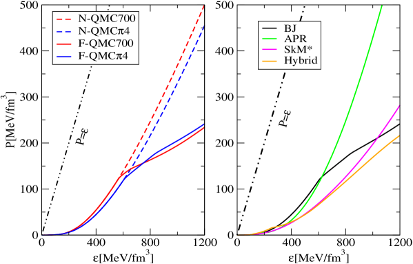
Figure 4: Left panel: Pressure as a function of total energy density for sample EoS for $\beta$-equilibrium matter containing nucleons p+n+e+$\mu$ (N-QMC700, N-QMC$\pi$4) and the full octet (F-QMC700, F-QMC$\pi$4). Right panel: Results of BJ, APR, SkM^∗ and hybrid EoS. The curve $P=\epsilon$ shows the stiffest possible EoS.

The calculated properties of neutron stars with the maximum mass for all 12 model EoS are summarised in Table 5. For comparison, the results for the BJ, APR, SkM^∗ and Hybrid EoS are also included. The same information is given for these models for stars with ‘canonical’ mass 1.4 M_⊙ in Table 6. It should be noted that the entries in Table 6 do not differ for the full octet and nucleon-only versions of the model, because the central density of 1.4 M_⊙ stars is below the threshold for the creation of hyperons.

Table 5: Parameters of maximum mass, cold neutron stars for the full set of QMC EoS. $n_{c}$ and $\rho_{c}$ are the central baryon number density [ fm^-3] and total mass density [$10^{15}$ g cm^-3] respectively, $R$ [km] is the radius, the maximum gravitational mass is M_⊙, $A$ [10⁵⁷] is the total baryon number, $E_{\rm bind}$ [10⁵³ erg] is the binding energy and $\tau$ [msec] is the estimate of the rotation period calculated from Eq. (42), $v_{\rm s}$ is the speed of sound and $z_{\rm surf}$ is the radiational red-shift. The index ‘max’ has been dropped for all observables in the header of this table.

EoS	$n_{\rm c}$	$\rho_{\rm c}$	$R$	$M_{\rm g}$	$A$	$E_{\rm bin}$	$\tau$	$v_{\rm s}$	$z_{\rm surf}$
F-QMC600	0.81	1.66	12.45	1.99	2.75	5.85	0.81	0.65	0.38
F-QMC700	0.82	1.68	12.38	1.98	2.74	5.85	0.80	0.65	0.38
F-QMC$\pi 1$	0.85	1.75	12.19	1.96	2.72	5.80	0.79	0.66	0.38
F-QMC$\pi 2$	0.86	1.79	12.08	1.93	2.66	5.56	0.78	0.65	0.38
F-QMC$\pi 3$	0.89	1.85	11.93	1.90	2.62	5.42	0.77	0.66	0.37
F-QMC$\pi 4$	0.93	1.93	11.70	1.85	2.54	5.17	0.76	0.66	0.37
N-QMC600	0.96	2.18	11.38	2.22	3.14	7.68	0.67	0.84	0.54
N-QMC700	0.96	2.19	11.34	2.21	3.14	7.69	0.67	0.84	0.54
N-QMC$\pi 1$	0.99	2.25	11.19	2.18	3.09	7.55	0.66	0.84	0.55
N-QMC$\pi 2$	1.01	2.31	11.08	2.15	3.04	7.31	0.65	0.84	0.55
N-QMC$\pi 3$	1.04	2.38	10.94	2.12	2.99	7.13	0.64	0.84	0.53
N-QMC$\pi 4$	1.09	2.49	10.73	2.07	2.91	6.84	0.63	0.84	0.53
BJ	1.31	3.04	9.92	1.851	2.56	5.41	0.60		0.49
APR	1.15	2.76	9.99	2.201	3.21	9.03	0.55	$>$1.00	0.69
SkM∗	1.66	3.83	8.94	1.617	2.22	4.47	0.55	0.82	0.46
Hybrid	1.33	2.81	10.42	1.453	1.93	3.02	0.72		0.30

Table 6: The same as Table 5 but for 1.4 M_⊙ star models. Data for N-QMCx EoS are not shown as they are identical to results of F-QMCx EoS because the central density of all 1.4 M_⊙ stars is predicted to be below the threshold for the appearance of hyperons.

EoS	$n_{\rm c}$	$\rho_{\rm c}$	$R$	$A$	$E_{\rm bin}$	$\tau$	$v_{\rm s}$	$z_{\rm surf}$
F-QMC600	0.39	0.69	12.94	1.86	2.76	1.02	0.58	0.21
F-QMC700	0.39	0.70	12.88	1.86	2.76	1.01	0.58	0.21
F-QMC$\pi 1$	0.41	0.73	12.74	1.86	2.79	0.99	0.58	0.22
F-QMC$\pi 2$	0.42	0.75	12.67	1.85	2.75	0.99	0.59	0.22
F-QMC$\pi 3$	0.43	0.78	12.55	1.85	2.75	0.97	0.59	0.22
F-QMC$\pi 4$	0.46	0.83	12.38	1.86	2.79	0.95	0.59	0.28
BJ	0.59	1.09	11.86	1.86	2.76	0.89		0.24
APR	0.55	1.00	11.47	1.87	3.03	0.85		0.29
SkM∗	0.87	1.68	10.51	1.88	3.12	0.74	0.62	0.25
Hybrid	0.91	1.79	11.20	1.86	2.76	0.82		0.28

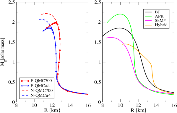
Figure 5: The gravitational masses of non-rotating neutron-star models (measured in solar masses) plotted against radius (in kilometers), calculated for selected QMC EoS – see the text for more explanation.

The relation between the gravitational mass and radius for various neutron star models is shown in Fig. 5, for a representative set of EoS, chosen to be F-QMC700, F-QMC$\pi 4$, N-QMC700 and N-QMC$\pi 4$.

Apart from the basic mass-radius relation, there are other features of neutron stars that provide the possibility to constrain the EoS and thus the nucleon-nucleon interaction in stellar matter. The volume and quality of the observational data has increased in recent years, offering more options for testing the physical basis of the EoS.

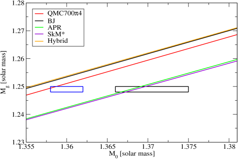
Figure 6: Relation between the gravitational mass, M_g, for various neutron star models (including the QMC EoS) and the corresponding baryonic mass, M₀. The boxes represent constraints derived by Podsiadlowski et al.[7] (black box) and more recently by Kitaura et al.[47] (blue box), based on the properties os system J0737-3039, as discussed in the text.

An important constraint on the EoS at relatively low densities has been recently identified [7] in connection with the very precise determination of the gravitational mass of Pulsar B in the system J0737-3039, $M_{\rm g}$ = 1.249$\pm$0.001 $M_{\odot}$. If the progenitor star was a white dwarf with O-Ne-M core and Pulsar B was formed in an electron-capture supernova, a possibility supported in part by new observations [48], a rather narrow range for the baryonic mass, $M_{\rm 0}$, between 1.366–1.375 $M_{\odot}$, can be determined for the pre-collapse core. Assuming that there is no (or negligible) baryon loss during the collapse, the newly born neutron star will have the same baryonic mass as the progenitor star. For any given EoS for cold neutron star matter the relation between the gravitational and baryonic mass can be calculated and tested against a very narrow window (full black line box in Fig. 6)defined by the data for Pulsar B. The width of the window reflects uncertainty in modelling the composition of the progenitor core, namely electron-capture rates, nuclear network calculation, Coulomb and general relativity corections. Very recently, another simulation of the explosion of O-Ne-Mg cores [47] has been performed which predicts the baryonic mass of Pulsar B 1.36$\pm$0.002 $M_{\odot}$ (full blue line box in Fig. 6). The error includes the uncertainty in the EoS used and the wind ablation after the simulation was terminated. This model (see Ref. [47]) includes a small mass loss between 0.014 to 0.017 $M_{\odot}$ in the process. As seen in Fig. 6, F-QMC$\pi$4 (the other versions give essentially the same curves) agrees with the latter constraint and predicts mass loss in the region of 0.008 - 0.017 $M_{\odot}$ in the model of Podsiadlowski et al [7], which is rather similar to the result of Kitaura et al [47]. The other sample EoSs either do not predict any mass loss (APR and SkM^∗) or they predict a mass loss which is too large.

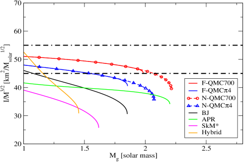
Figure 7: Moment of inertia, scaled by $M^{\rm 3/2}$, as a function of the stellar mass, $M$, for sample QMC EoS. The BJ, APR, SkM^∗ and Hybrid EoS results are added for comparison. The dash-dot lines indicate the predicted experimental constraints from Ref. [6] - see the text for details.

Another interesting possibility has been recently suggested by Lattimer and Schultz [6]. Measurement of the moment of inertia of Pulsar A (with known mass of about 1.34 M_⊙) in the same system, to $\sim$10% precision, would allow a rather accurate estimate of the radius of the star and of the pressure in matter of density in the vicinity of $1\div 2n_{\rm 0}$. Such information could provide a rather strong constraint on the EoS of neutron stars. In Fig. 7, using exactly the same scale as as Fig. 1 of Ref. [6], we illustrate this possibility. The dashed horizontal lines depict the error range of a hypothetical result of a measurement, selected as close as possible to the expected value. If this were the actual experimental result, many EoS would not be useful in determining the radius of Pulsar A, as they would cross the area between the two dashed lines either below or above M = 1.34 M_⊙. The QMC EoS would satisfy this constraint. Moreover, their relatively weak mass dependence would be an advantage in the study of of another analogous system with known mass up to $\sim$1.6 M_⊙ (N-QMC$\pi$4) and $\sim$2 M_⊙. We note that incorporation of hyperons shortens this range at higher masses, as illustrated in Fig. 7.

Finally, we study the implications of the baryon composition of stellar matter, as calculated using the sample EoS, for a possible cooling mechanism of neutron stars either just after their birth in supernovae or after heating in an accretion episode. The cooling mechanisms can, in principle, provide further important constraints on neutron-star models. However, as discussed in more detail previously [44], the cooling processes for both young and old neutron stars are not currently known with any certainty, although several scenarios have been proposed [49, 50]. Many of them involve emission of neutrinos from the stellar core. The most frequently discussed, the direct URCA process, produces neutrinos in proton-neutron weak decays with an additional production of either electrons of muons. The proton concentration in the matter is a crucial ingredient of the process. Conservation of energy and momentum requires $y^{1/3}_{\rm n}<y^{1/3}_{\rm p}+y^{1/3}_{\rm e}$, or $y^{1/3}_{\rm n}<y^{1/3}_{\rm p}+y^{1/3}_{\rm\mu}$, to be satisfied. This, in turn, can happen only in matter where the proton fraction grows steadily with increasing density and $y_{p}$ is greater than about 0.11 for matter consisting of only protons, neutrons and electrons. Medium effects and additional interactions among the particles change this number only slightly [46] but the presence of muons increases the critical ratio, $y_{p}$, to about 0.15. We display the proton fraction for sample EoS in Fig. 8. It is clear that the proton fraction in F-QMC700 and F-QMC$\pi 4$ pass this critical limit at densities close to $0.6{\rm\ fm}^{-3}$, coincident with the appearence of negative $\Xi^{-}$ hyperons. This density is well below the central density for maximum mass models and thus the direct URCA process is allowed for models of astrophysical interest, in agreement with expectation. On the contrary, for the N-QMC700 and N-QMC$\pi 4$ models the critical density for the start of the direct URCA process is much higher, between $0.8\div 1.0{\rm\ fm}^{-3}$, and is close to or exceeds the inferred maximum central density, suggesting that this cooling mechanism would not be allowed in these cases. This reinforces our message concerning the importance of incorporating of the full baryon octet in QMC.

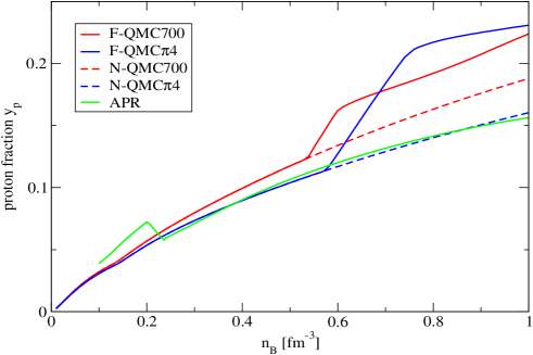
Figure 8: The proton fraction $y_{\rm p}$ for beta stable matter, as calculated using the QMC EoS is plotted as a function of the baryon number density $n_{B}$. The data for the APR EoS are added for comparison.

6 Conclusions

One of the most important features of the QMC EoS is that although the QMC and Skyrme energy functionals have similar structure at densities close to nuclear saturation density, they differ significantly at higher densities, because of their different density and isospin dependence. The QMC EoS provide cold neutron star models with maximum mass 1.9–2.1 M_⊙, with central density less than 6 times nuclear saturation density and thus offer a consistent description of the stellar mass up to this density limit, without extrapolation beyond the region of validity – as needed, for example, when the non-relativistic, nucleon-only Skyrme models are used at these densities. The maximum mass of neutron stars in the QMC model is close to the most recent observation, the central density is relatively low in comparison to other models and all the predicted stars are well within the causal limit.

The QMC model includes self-consistently the presence of hyperons at high densities. Unlike most other models, no hyperon contribution at densities lower than $3\,n_{0}$ is predicted in $\beta$-equilibrium matter. At higher densities, $\Xi^{-,0}$ and $\Lambda$ hyperons are present. The absence of the $\Sigma^{\rm\pm,0}$ hyperons is due, on the one hand, to the unique features of the model, namely the implementation of the color hyperfine interaction and the scalar polarisability of the baryons and, on the other hand, to the use of the Hartree-Fock approximation. The pronounced effects of the presence of hyperons on the properties of dense matter and neutron star models have been identified by a comparison of nucleon-only EoS with full-baryon-octet EoS. In nuclear matter, the presence of hyperons, as expected, softens the EoS as illustrated in Fig. 4. However, it needs to be stressed that the composition of stellar matter at high density is not necessarily the only determining factor of the behaviour of pressure with increasing density. In fact, it is critically dependent on the potentials acting amongst particles present in the matter.

In neutron star models, the hyperon component systematically reduces the prediction of the maximum mass of a neutron star and increases its radius at maximum mass, as demonstrated in Fig. 5. This is a very important finding, because many non-relativistic EoS, including those based on the effective Skyrme interaction and the A18+$\delta$v+UIX^∗ potential, do not include hyperons at densities corresponding to the central density of maximum mass star models and thus their results should be taken with caution. Moreover, the relationship between the moment of inertia and the stellar gravitational mass, $M_{\rm g}$, is clearly influenced (see Fig. 7), as is the cooling mechanism expected to take place in neutron stars - the direct URCA process - is predicted to be allowed in stars with hyperons but not in nucleon-only neutron stars. It is also important to realise that the models for the nucleon-hyperon and hyperon-hyperon interactions play an important role in this comparison. In future, it would be interesting to apply the present QMC model to non-equilibrium matter at finite temperature and produce EoS that could be tested in core-collapse supernova simulation models. The high density threshold for the appearance of hyperons probably rules out any hyperon-related effects taking place in the collapsing star at the bounce density of $1.5-2.0\,n_{0}$, in variance with some other EoS with a much lower threshold density (e.g. [51]).

7 Acknowledgement

This work has been supported by US DOE grant DE-FG02-94ER40834 and by US DEO grant DE-AC05-06OR23177, under which Jefferson Science Associates operates Jefferson Lab and by the Espace de Structure Nucléaire Théorique du CEA. (JRS) wishes to acknowledge helpful discussions with P. Podsiadlowski and J. C. Miller and to thank J. C. Miller for providing a code for calculation of properties of slowly rotating neutron stars.

8 Appendix

8.1 Free mass of the baryons in the bag model

The free mass of the baryon of flavor $f$ with quark content $(N_{ud},N_{s})$ is written as

$$M_{f}=\frac{N_{ud}\Omega(m_{ud})+N_{s}\Omega(m_{s})}{R}-\frac{Z_{0}}{R}+\Delta E_{M}(f)+\frac{4\pi BR^{3}}{3}$$ (44)

where the quark mode $\Omega(m)$ is determined by the boundary condition

$$\frac{\sin x}{x}+\frac{1}{\Omega+mR}\left(\cos x-\frac{\sin x}{x}\right)=0,\,\,\,\,x=\sqrt{\Omega^{2}-(mR)^{2}}$$ (45)

and $B$ is the bag constant. In the presence of the scalar field one can have $\Omega^{2}-(mR)^{2}<0$ but the equation remains valid by analytical continuation. The bag radius is fixed for each flavour by the stability condition

$$\frac{\partial M_{f}}{\partial R}=0.$$ (46)

We set the $u,d$ mass equal to zero and the zero point parameter $Z_{0}$ is assumed to be the same for all particles. For completeness we briefly recall how the hyperfine color interaction $\Delta E_{M}$ is evaluated according to [52]. For a color singlet baryon one has

$$\Delta E_{M}=\sum_{i<j}E_{ij}\vec{\sigma_{i}}.\vec{\sigma_{j}}$$ (47)

with $\vec{\sigma_{i}}$ the Pauli spin matrices of the $i^{th}$ quark and

$$E_{ij}=8\alpha_{c}\frac{\mu_{i}(R)\mu_{j}(R)}{R^{3}}I_{ij}$$ (48)

where $\alpha_{c}$ is the color coupling constant. The magnetic moment has the expression

$$\mu_{i}(R)=\frac{R}{6}\frac{4\Omega(m_{i})+2Rm_{i}-3}{2\Omega(m_{i})\left(\Omega(m_{i})-1\right)+Rm_{i}}.$$ (49)

and we point out that its quark mass dependence will produce a non trivial flavor dependence of the coupling to the nuclear scalar field. The expression for the overlap integral $I_{ij}$ is:

$$I_{ij} = 1+\frac{-3y_{i}y_{j}-4x_{i}x_{j}\sin^{2}x_{i}\sin^{2}x_{j}+x_{i}x_{j}K_{ij}}{2(x_{i}\sin^{2}x_{i}-\frac{3}{2}y_{i})(x_{j}\sin^{2}x_{j}-\frac{3}{2}y_{j})}$$ (50)

$$K_{ij} = 2x_{i}Si(2x_{i})+2x_{j}Si(2x_{j})$$ (52)

$$-(x_{i}+x_{j})Si(2x_{i}+2x_{j})-(x_{i}-x_{j})Si(2x_{i}-2x_{j})$$

$$y_{i} = x_{i}-\sin x_{i}\cos x_{i},\,\,\,x_{i}=\sqrt{\Omega(m_{i})^{2}-(Rm_{i})^{2}}$$ (53)

Using the spin-flavor wave functions of the baryons one can write:

$$\Delta E_{M}=a_{00}E_{00}+a_{0s}E_{0s}+a_{ss}E_{ss}$$ (54)

where the index 0 refers to the $u,d$ quarks ans $s$ to the strange quark. The spin-flavor factors $a_{ii}$ are given in Table 7.

	$a_{00}$	$a_{0s}$	$a_{ss}$
N	-3	0	0
$\Lambda$	-3	0	0
$\Sigma$	1	-4	0
$\Xi$	0	-4	1

Table 7: Spin-flavor factors for Eq.(54)

To fix the free parameters $(B,Z_{0},m_{s},\alpha_{c})$ we take the free nucleon radius $R_{N}^{free}$ as the free parameter and require that the nucleon and $\Delta(1232)$ have their physical masses. Together with the stability equations this determines $(B,Z_{0},\alpha_{c})$. We then choose $m_{s}$ so as to have a best fit to the $(\Lambda,\Sigma)$ masses. The resulting parameters are shown in Table 8 for typical values of $R_{N}^{free}$.

$R_{N}^{free}({\rm\ fm})$	$B({\rm\ fm}^{-4})$	$Z_{0}$	$\alpha_{c}$	$m_{s}({\rm\ MeV})$
0.8	0.554	2.642	0.448	341
1.0	0.284	1.770	0.560	326

Table 8: Values of the parameters $(B,Z_{0},m_{s},\alpha_{c})$ for typical values of $R_{N}^{free}$.

8.2 Effective mass

We now consider the effect of the nuclear scalar field which is assumed to be constant over the volume of the baryon. We recall that the variation of the field just produces the spin-orbit interaction, which we can neglect when considering uniform matter. Let $\sigma$ be the uniform value of the scalar field and $g_{\sigma}^{q}$ its coupling to the $u,d$ quarks. We assume that the strange quark does not interact with the scalar field. Therefore the coupling to the scalar field amounts to the substitution

$$m_{ud}\rightarrow m_{ud}-g_{\sigma}^{q}\sigma,\,\,\,m_{s}\rightarrow m_{s}$$ (55)

in the free mass equation, Eq. (44), followed by application of the stability condition to determine the actual radius. The mass then becomes a function of $\sigma$ and of the parameters, $(B,Z_{0},m_{s},\alpha_{c})$, which themselves depend only on $R_{N}^{free}$. So we have

$$M_{f}({\rm in\,medium})\equiv M_{f}(m_{ud}-g_{\sigma}^{q}\sigma,R_{N}^{free})$$ (56)

Since we have two independent energy scales, $\sigma$ and $1/R_{N}^{free}$, dimensional analysis is not very helpful and we simply make a fit of $M_{f}(\sigma,R_{N}^{free})-M_{f}(0,R_{N}^{free})$ in powers of $m_{ud}-g_{\sigma}^{q}\sigma$, with the coefficients also fitted as polynomials in $R_{N}^{free}$. We then define the free $\sigma-N$ coupling as

$$g_{\sigma}=\left.\frac{\partial M_{N}(\sigma,R_{N}^{free})}{\partial\sigma}\right|_{\sigma=0}=-g_{\sigma}^{q}\left.\frac{\partial M_{N}(\sigma,R_{N}^{free})}{\partial m}\right|_{m=0}$$ (57)

which allows us to eliminate $g_{\sigma}^{q}$ in favor of $g_{\sigma}$. We then get an expansion of the form

$$M_{f}(\sigma,R_{N}^{free})-M_{f}(0,R_{N}^{free})=P_{f}^{(1)}(R_{N}^{free})g_{\sigma}\sigma+P_{f}^{(2)}(R_{N}^{free})(g_{\sigma}\sigma)^{2}+....$$ (58)

where, by construction

$$P_{N}^{(1)}(R_{N}^{free})=-1.$$ (59)

If the mass were approximated by

$$M_{f}=\frac{N_{u,d}\Omega(m_{ud})+N_{s}\Omega(m_{s})}{R_{N}^{free}}$$ (60)

we would have

$$P_{\Lambda\Sigma}^{(1)}=-2/3,\,\,\,P_{\Xi}^{(1)}=-1/3,$$ (61)

but this approximation is severely broken in the realistic case. The order of the polynomials in $R$ has been set to 2 and the coefficients have been fitted over the range $[0.7{\rm\ fm}\rightarrow 1.3{\rm\ fm}].$ We have checked that an expansion truncated at order $\left(g_{\sigma}\sigma\right)^{2}$ was sufficient, even for scalar fields as large as $g_{\sigma}\sigma=600{\rm\ MeV}$. This corresponds to densities of order $1{\rm\ fm}^{-3}$, which is sufficient for our purposes. The expansion becomes, with everything expressed in ${\rm\ fm}$:

$$M_{N}(\sigma) = M_{N}-g_{\sigma}\sigma$$ (62)

$$+\left[0.0022+0.1055R_{N}^{free}-0.0178\left(R_{N}^{free}\right)^{2}\right]\left(g_{\sigma}\sigma\right)^{2}$$

$$M_{\Delta}(\sigma) = M_{\Delta}-\left[0.9957-0.22737R_{N}^{free}+0.01\left(R_{N}^{free}\right)^{2}\right]g_{\sigma}\sigma$$ (63)

$$+\left[0.0022+0.1235R_{N}^{free}-0.0415\left(R_{N}^{free}\right)^{2}\right]\left(g_{\sigma}\sigma\right)^{2}$$

$$M_{\Lambda}(\sigma) = M_{\Lambda}-\left[0.6672+0.0462R_{N}^{free}-0.0021\left(R_{N}^{free}\right)^{2}\right]g_{\sigma}\sigma$$ (64)

$$+\left[0.0016+0.0686R_{N}^{free}-0.0084\left(R_{N}^{free}\right)^{2}\right]\left(g_{\sigma}\sigma\right)^{2}$$

$$M_{\Sigma}(\sigma) = M_{\Sigma}-\left[0.6706-0.0638R_{N}^{free}-0.008\left(R_{N}^{free}\right)^{2}\right]g_{\sigma}\sigma$$ (65)

$$+\left[-0.0007+0.0786R_{N}^{free}-0.0181\left(R_{N}^{free}\right)^{2}\right]\left(g_{\sigma}\sigma\right)^{2}$$

$$M_{\Xi}(\sigma) = M_{\Xi}-\left[0.3395+0.02822R_{N}^{free}-0.0128\left(R_{N}^{free}\right)^{2}\right]g_{\sigma}\sigma$$ (66)

$$+\left[-0.0014+0.0416R_{N}^{free}-0.0061\left(R_{N}^{free}\right)^{2}\right]\left(g_{\sigma}\sigma\right)^{2}$$

Note that in these calculations we use the physical masses for the free particles. The influence of the bag model dependence then appears only in the interaction piece, $M_{f}(\sigma)-M_{f}(0)$. It is convenient to write the dynamical mass in the form

$$M_{f}(\sigma)=M_{f}-w_{f}^{\sigma}g_{\sigma}\sigma+\frac{d}{2}\tilde{w}_{f}^{\sigma}\left(g_{\sigma}\sigma\right)^{2}$$ (67)

where the scalar polarisability, $d$, and the dimensionless weights, $w_{f}^{\sigma},\tilde{w}_{f}^{\sigma}$, are deduced from Eqs. (62-66). For illustrative purposes we give their values in Table 9 for our preferred value of the free radius, $R_{N}^{free}=0.8{\rm\ fm}$.

	$N$	$\Lambda$	$\Sigma$	$\Xi$
d$({\rm\ fm})$	0.15	0.15	0.15	0.15
$w_{f}^{\sigma}$	1	0.703	0.614	0.353
$\tilde{w}_{f}^{\sigma}$	1	0.68	0.673	0.371

Table 9: The weights for $R_{N}^{free}=0.8{\rm\ fm}$.

References

- [1] J. M. Lattimer and M. Prakash. Phys. Rep., 334:121, 2000.
- [2] H. Heiselberg and M. Hjorth-Jensen. Phys. Rep., 328:328, 2000.
- [3] J. M. Lattimer and M. Prakash. ApJ, 550:426, 2001.
- [4] J. Rikovska Stone, J. C. Miller, R. Koncewicz, P. D. Stevenson, and M. R. Strayer. Phys. Rev., C68:034324, 2003.
- [5] J. M. Lattimer and M. Prakash. Phys. Rev. Lett., 94:111101, 2005.
- [6] J. M. Lattimer and B. F. Schultz. ApJ, 629:979, 2005.
- [7] Ph. Podsiadlowski, J. D. M. Dewi, P. Lesaffre, J. C. Miller, W. G. Newton, and J. R. Stone. Mon. Not. R. Astron. Soc., 361:1243, 2005.
- [8] T. Klahn et al. PR, C74:035802, 2006.
- [9] Fridolin Weber. Strange quark matter and compact stars. Prog. Part. Nucl. Phys., 54:193–288, 2005, astro-ph/0407155.
- [10] Jurgen Schaffner-Bielich. Strange quark matter in stars: A general overview. J. Phys., G31:S651–S658, 2005, astro-ph/0412215.
- [11] Tomoyuki Maruyama, Takumi Muto, Toshitaka Tatsumi, Kazuo Tsushima, and Anthony W. Thomas. Kaon condensation and lambda nucleon loop in the relativistic mean-field approach. Nucl. Phys., A760:319–345, 2005, nucl-th/0502079.
- [12] Toshitaka Tatsumi. Kaon condensation and neutron stars. Prog. Theor. Phys. Suppl., 120:111–134, 1995.
- [13] S. Lawley, W. Bentz, and A. W. Thomas. Nucleons, nuclear matter and quark matter: A unified NJL approach. J. Phys., G32:667–680, 2006, nucl-th/0602014.
- [14] S. Lawley, W. Bentz, and A. W. Thomas. The phases of isospin asymmetric matter in the two flavor NJL model. Phys. Lett., B632:495–500, 2006, nucl-th/0504020.
- [15] P. A. M. Guichon and A. W. Thomas. Phys. Rev. Lett., 93:132502, 2004.
- [16] P. A. M. Guichon, H. H. Matevosyan, N. Sandulescu, and A. W. Thomas. Nucl. Phys., A772:1, 2006.
- [17] P. A. M. Guichon. Phys. Lett., B200:235, 1998.
- [18] F. Bissey et al. Nucl. Phys. Proc. Suppl., 141:22–25, 2005, hep-lat/0501004.
- [19] P. A. M. Guichon, K. Saito, E. N. Rodionov, and A. W. Thomas. Nucl. Phys., A601:349, 1996.
- [20] G. Krein, Anthony W. Thomas, and K. Tsushima. Nucl. Phys., A650:313–325, 1999, nucl-th/9810023.
- [21] Anthony W. Thomas. Chiral symmetry and the bag model: A new starting point for nuclear physics. Adv. Nucl. Phys., 13:1–137, 1984.
- [22] G. Chanfray. private communication.
- [23] N. K. Glendenning. In Compact Stars. Springer, Berlin, Heidelberg, New York, 2000.
- [24] W. D. Arnett and R. L. Bowers. Astrophys. J. Supplement, 33:415, 1977.
- [25] V. R. Pandharipande. Nucl. Phys., A178:123, 1971.
- [26] S. Balberg, I. Lichtenstadt, and G. B. Cook. Astrophys. J. Supplement, 121:515, 1999.
- [27] R. B. Wiringa. Rev. Mod. Phys., 65:231, 1993.
- [28] F. Hofmann, C.M. Keil, and H. Lenske. Phys. Rev., C64:025804, 2001.
- [29] K. Iida and K. Sato. Phys. Rev., C58:2538, 1998.
- [30] G. F. Burgio, P. K. Sahu M. Baldo, and H.-J. Schulze. Phys. Rev., C66:025802, 2002.
- [31] D. P. Menezes and C. Providencia. Phys. Rev., C68:035804, 2003.
- [32] G. Baym, H. Bethe, and C. Pethick. Nucl. Phys., A175:225, 1971.
- [33] G. Baym, C. Pethick, and P. Sunderland. ApJ, 170:299, 1971.
- [34] D. J. Nice, E. M. Splaver, I. H. Stairs, O. Löhmer, A. Jessner, M. Kramer, and J. M. Cordes. ApJ, 634:1242, 2005.
- [35] A. Akmal, V. R. Pandharipande, and D. G. Ravenhall. Phys. Rev., C58:1804, 1998.
- [36] E. Chabanat, P. Bonche, P. Hansel, J. Meyer, and R. Schaeffer. Nucl. Phys., A627:710, 1997.
- [37] R. C. Tolman. Proc. Natl. Acad. Sci. USA, 20:3, 1934.
- [38] J. R. Oppenheimer and G. M. Volkov. Phys. Rev., 55:374, 1939.
- [39] R. Schaffer, Y. Declais, and S. Julian. Nature, 300:142, 1987.
- [40] J. W. T. Hessels, S. C. Ransom, I. H. Stairs, P. C. C. Freire, V. M. Kaspi, and F. Camilo. Science, 311:1901, 2006.
- [41] P. Haensel and J. L. Zdunik. Nature (London), 340:617, 1989.
- [42] P. Haensel, M. Salgado, and S. Bonazzola. Astron. Astrophys., 296:745, 1994.
- [43] J. B. Hartle. ApJ, 150:1005, 1967.
- [44] J. Rikovska Stone, P. D. Stevenson, J. C. Miller, and M. R. Strayer. Phys. Rev., C65:064213, 2002.
- [45] H. A. Bethe and M. B. Johnson. Nucl. Phys., A230:1, 1974.
- [46] D. Page, U. Geppert, and F. Weber. in print in Nucl. Phys. A, 2006.
- [47] F. S. Kitaura, H.-Th. Janka, and W. Hillebrant. 2006.
- [48] H. Stairs, S. E. Thorsett, R. J. Dewey, M. Kramer, and C. A. McPhee. 2006.
- [49] D. Page, J. M. Lattimer, M. Prakash, and A. W. Steiner. Astrophys. J. Suppl., 155:623, 2004.
- [50] P. B. Jones. Phys. Rev., D64:084003, 2001.
- [51] D. P. Menezes and C. Providencia. Phys. Rev., C69:045801, 2004.
- [52] Thomas A. DeGrand, R. L. Jaffe, K. Johnson, and J. E. Kiskis. Phys. Rev., D12:2060, 1975.