Shell model method for Gamow-Teller Transitions in heavy, deformed nuclei

Abstract

A method for calculation of Gamow-Teller transition rates is developed by using the concept of the Projected Shell Model (PSM). The shell model basis is constructed by superimposing angular-momentum-projected multi-quasiparticle configurations, and nuclear wave functions are obtained by digonalizing the two-body interactions in these projected states. Calculation of transition matrix elements in the PSM framework is discussed in detail, and the effects caused by the Gamow-Teller residual forces and by configuration-mixing are studied. With this method, it may become possible to perform a state-by-state calculation for $\beta$-decay and electron-capture rates in heavy, deformed nuclei at finite temperatures. Our first example indicates that, while experimentally known Gamow-Teller transition rates from the ground state of the parent nucleus are reproduced, stronger transitions from some low-lying excited states are predicted to occur, which may considerably enhance the total decay rates once these nuclei are exposed to hot stellar environments.

I Introduction

The knowledge on weak interaction processes is one of the most important ingredients for resolving astrophysical problems. The first systematical work on stellar weak-interaction rates was performed by Fuller, Fowler, and Newman FFN1 ; FFN2 ; FFN3 ; FFN4 , who recognized the decisive role played by the Gamow-Teller (GT) transitions. Due to their pioneering work, the study of stellar weak interaction rates requested by astrophysics becomes essentially a nuclear structure problem, in which the actual decay rates are determined by the microscopic inside of nuclear many-body systems. It has been suggested that the nuclear shell model, i.e. a full diagonalization of an effective Hamiltonian in a chosen model space, is the most preferable method for GT transition calculations. This was noticed early by Aufderheide et al. ABRM93 , and has recently been emphasized by Langanke and Martínez-Pinedo LM03 .

For a theoretical model employed in GT transition calculations, it is generally required that the model can reproduce a wide range of structure properties of relevant nuclei. It has been shown that the state-of-the-art shell-model diagonalization method is indeed capable of performing such calculations. For example, Wildenthal and Brown Wild84 ; BW85 obtained nuclear wave functions in the full $sd$-shell model space, which were successfully applied to calculation of GT rates in the $sd$ shell nuclei Oda94 . By using the method developed by the Strasbourg-Madrid group SM94 , Langanke and Martínez-Pinedo LM01 made the shell-model GT rates available also for the $pf$ shell nuclei. Still, these sophisticated calculations are tractable only for nuclei up to the mass-60 region, and cannot be applied to heavier nuclei which play important roles in the nuclear processes in massive stars.

In the long history of the nuclear shell-model development, tremendous effort has been devoted to extending the shell-model capacity from its traditional territory to heavier shells. Despite the great progress made in recent years, it seems impossible to treat an arbitrarily large nuclear system in a spherical shell model framework due to the unavoidable problem of dimension explosion. One is thus compelled to seek judicious schemes to deal with large nuclear systems. The central issue has been the shell-model truncation. There are many different ways of truncating a shell-model space. While in principle, it does not matter how to prepare a model basis, it is crucial in practice to use the most efficient one. In this regard, we recognize the fact that except for a few lying in the vicinity of shell closures, most nuclei in the nuclear chart are deformed. This naturally suggests for a shell model calculation to use a deformed basis to incorporate the physics in large systems. That is the philosophy that the Projected Shell Model (PSM) PSM and the several important generalizations Sheikh99 ; Chen01 ; Sun02 ; Sun03 ; Gao06 are based on.

The present article reports on the new development for calculation of GT transition rates in the PSM framework. Before a detailed description of the work, we mention a few attractive features in our approach, which may be relevant for future astrophysical applications.

• The PSM utilizes single particle bases generated by deformed mean-field models yet carries out a shell-model diagonalization like the conventional shell model. Conceptually, the PSM bridges two important nuclear structure methods: the deformed mean-field approach and the conventional shell model, and takes the advantages of both. On the one hand, as a shell model, the PSM can be applied to any heavy, deformed nuclei without a size limitation. On the other hand, unlike the mean-field models or models with an average nature, the PSM wave functions contain correlations beyond mean-field and the states are written in the laboratory frame having definite quantum numbers such as angular-momentum and parity. These are needed properties when the wave functions are employed in transition calculations.

• Because of the way the PSM constructs its basis, the dimension of the model space is small (usually in the range of $10^{2}-10^{4}$). With this size of basis, a state-by-state evaluation of GT transition rates is computationally feasible. This feature is important because in stellar environments with finite temperatures, the usual situation is that the thermal population of excited states in a parent nucleus sets up connections to many states in a daughter by the GT operator. However, our current knowledge on GT transitions from excited nuclear states is very poor, and in many cases, it must rely on theoretical calculations.

• The calculation of forbidden transitions involves nuclear transitions between different harmonic oscillator shells and thus requires multi-shell model spaces. Such a calculation is not feasible for most of the conventional shell models working in one-major shell bases. The PSM is a multi-shell shell model. This feature is desired particularly when forbidden transitions are dominated.

• Isomeric states belong to a special group of nuclear states because of their long half-lives. The existence of isomeric states in nuclei could alter significantly the elemental abundances produced in nucleosynthesis. There are cases in which an isomer of sufficiently long lifetime can change the paths of reactions taking place and lead to a different set of elemental abundances Sun05a ; Sun05b . It has been shown that the PSM is indeed capable of describing the detailed structure of isomeric states Sun04 .

The paper is organized as follows. In Sec. II, we briefly introduce the PSM concept and describe how shell model diagonalization is carried out in the angular-momentum-projected bases. Technical details of calculation of transition matrix elements in the projected bases are given in Sec. III. Our first example of a GT transition calculation is illustrated in Sec. IV, where we first validate the model by comparing the calculated structure properties (energy levels and electromagnetic transitions) with experiment. The obtained GT transition results are then discussed and the effects caused by the Gamow-Teller residual forces and by configuration mixing are studied. Finally, the work is summarized and an outlook on future applications is given in Sec. V.

II Outline of the model

The Projected Shell Model PSM works with the following scheme. It begins with the deformed Nilsson single particle basis, with pairing correlations incorporated into the basis by a BCS calculation for the Nilsson states. The Nilsson-BCS calculation defines a deformed quasiparticle (qp) basis. Then the angular-momentum (and if necessary, also particle-number, parity) projection is performed on the qp basis to form a shell model space in the laboratory frame. Finally a two-body Hamiltonian is diagonalized in this projected space.

Let $\left|\Phi\right>$ be the qp vacuum and $a^{\dagger}_{\nu}$ and $a^{\dagger}_{\pi}$ the qp creation operators, with the index $\nu$ ($\pi$) denoting the neutron (proton) quantum numbers and running over selected single-qp states for each configuration. The multi-qp configurations of the PSM are given for the four kinds of nuclei as follows:

$$\begin{array}[]{rl}\mbox{e-e:}&\{\left|\Phi\right\rangle,a^{\dagger}_{\nu_{i}}a^{\dagger}_{\nu_{j}}\left|\Phi\right\rangle,a^{\dagger}_{\pi_{i}}a^{\dagger}_{\pi_{j}}\left|\Phi\right\rangle,a^{\dagger}_{\nu_{i}}a^{\dagger}_{\nu_{j}}a^{\dagger}_{\pi_{k}}a^{\dagger}_{\pi_{l}}\left|\Phi\right\rangle,\cdots\},\vspace{4pt}\\ \mbox{odd-$\nu$:}&\{a^{\dagger}_{\nu_{i}}\left|\Phi\right\rangle,a^{\dagger}_{\nu_{i}}a^{\dagger}_{\nu_{j}}a^{\dagger}_{\nu_{k}}\left|\Phi\right\rangle,a^{\dagger}_{\nu_{i}}a^{\dagger}_{\pi_{j}}a^{\dagger}_{\pi_{k}}\left|\Phi\right\rangle,a^{\dagger}_{\nu_{i}}a^{\dagger}_{\nu_{j}}a^{\dagger}_{\nu_{k}}a^{\dagger}_{\pi_{l}}a^{\dagger}_{\pi_{m}}\left|\Phi\right\rangle,\cdots\},\vspace{4pt}\\ \mbox{odd-$\pi$:}&\{a^{\dagger}_{\pi_{i}}\left|\Phi\right\rangle,a^{\dagger}_{\pi_{i}}a^{\dagger}_{\nu_{j}}a^{\dagger}_{\nu_{k}}\left|\Phi\right\rangle,a^{\dagger}_{\pi_{i}}a^{\dagger}_{\pi_{j}}a^{\dagger}_{\pi_{k}}\left|\Phi\right\rangle,a^{\dagger}_{\pi_{i}}a^{\dagger}_{\pi_{j}}a^{\dagger}_{\pi_{k}}a^{\dagger}_{\nu_{l}}a^{\dagger}_{\nu_{m}}\left|\Phi\right\rangle,\cdots\},\vspace{4pt}\\ \mbox{o-o:}&\{a^{\dagger}_{\nu_{i}}a^{\dagger}_{\pi_{j}}\left|\Phi\right\rangle,a^{\dagger}_{\nu_{i}}a^{\dagger}_{\nu_{j}}a^{\dagger}_{\nu_{k}}a^{\dagger}_{\pi_{l}}\left|\Phi\right\rangle,a^{\dagger}_{\nu_{i}}a^{\dagger}_{\pi_{j}}a^{\dagger}_{\pi_{k}}a^{\dagger}_{\pi_{l}}\left|\Phi\right\rangle,a^{\dagger}_{\nu_{i}}a^{\dagger}_{\nu_{j}}a^{\dagger}_{\nu_{k}}a^{\dagger}_{\pi_{l}}a^{\dagger}_{\pi_{m}}a^{\dagger}_{\pi_{n}}\left|\Phi\right\rangle,\cdots\}.\end{array}$$ (1)

Note that the PSM works with multiple harmonic-oscillator shells for both neutrons and protons. The indices $\nu$ and $\pi$ in (1) are general; for example, a 2-qp state can be of positive parity if both quasiparticles $i$ and $j$ are from the major $N$-shells that differ in $N$ by $\Delta N=0,2,\dots$, or of negative parity if $i$ and $j$ are from those $N$-shells that differ by $\Delta N=1,3,\dots$. In bases (1), “$\cdots$” denotes those configurations having a higher order of quasiparticles, which may practically be ignored in the present study. On the other hand, the bases (1) can be easily enlarged if necessary. If the configurations denoted by “$\cdots$” are completely included, one recovers the full shell model space written in the representation of qp excitation.

The shell model basis states can then be constructed by the projection technique. Without losing generality, the PSM wave-function can be written as

$$\left|\Psi^{\sigma}_{IM}\right>=\sum_{K\kappa}f^{\sigma}_{IK_{\kappa}}\,\hat{P}^{I}_{MK}\left|\Phi_{\kappa}\right>,$$ (2)

where $\left|\Phi_{\kappa}\right\rangle$ denotes the qp-basis given in (1), and

$$\hat{P}^{I}_{MK}=\frac{2I+1}{8\pi^{2}}\int d\Omega D^{I}_{MK}(\Omega)\hat{R}(\Omega)$$ (3)

is the angular momentum projection operator RS80 . In Eq. (3), $D^{I}_{MK}$ is the $D$-function Ed60 , $\hat{R}$ the rotation operator, and $\Omega$ the solid angle. If one keeps the axial symmetry in the deformed basis, $D^{I}_{MK}$ in Eq. (3) reduces to the small $d$-function and the three dimensions in $\Omega$ reduce to one. The energies and wave functions (given in terms of the coefficients $f^{\sigma}_{IK_{\kappa}}$ in Eq. (2)) are obtained by solving the following eigen-value equation:

$$\sum_{K^{\prime}\kappa^{\prime}}(H_{K\kappa,K^{\prime}\kappa^{\prime}}^{I}-E^{\sigma}_{I}N_{K\kappa,K^{\prime}\kappa^{\prime}}^{I})f^{\sigma}_{IK_{\kappa^{\prime}}}=0$$ (4)

where $H^{I}_{K\kappa,K^{\prime}\kappa^{\prime}}$ and $N^{I}_{K\kappa,K^{\prime}\kappa^{\prime}}$ are respectively the matrix elements of the Hamiltonian and the norm

$$\begin{array}[]{rcl}H_{K\kappa,K^{\prime}\kappa^{\prime}}^{I}&=&\langle\Phi_{\kappa}|\hat{H}\hat{P}^{I}_{KK^{\prime}}|\Phi_{\kappa^{\prime}}\rangle\vspace{6pt}\\ N_{K\kappa,K^{\prime}\kappa^{\prime}}^{I}&=&\langle\Phi_{\kappa}|\hat{P}^{I}_{KK^{\prime}}|\Phi_{\kappa^{\prime}}\rangle.\end{array}$$ (5)

The PSM uses a large single-particle space, which ensures that the collective motion and the cross-shell interplay are defined microscopically by accommodating a sufficiently large number of active nucleons. It usually includes three (four) major harmonic-oscillator shells each for neutrons and protons in a calculation for deformed (superdeformed or superheavy) nuclei. However, the shell model dimension in Eq. (2) is small. This means that each of the configurations in (2) is a complex combination of spherical shell model basis states. Although the dimension where the final diagonalization is carried out is small, it is huge in terms of original shell model configurations. In this sense, the PSM is truly a shell model in a truncated multi-major-shell space.

The Hamiltonian in the present study consists of the separable forces

$$\hat{H}=\hat{H}_{0}+\hat{H}_{QP}+\hat{H}_{GT},$$ (6)

which represent different kinds of characteristic correlations between valence particles. It has the single-particle term $\hat{H}_{0}$, the quadrupole+pairing force $\hat{H}_{QP}$ with inclusion of the quadrupole-pairing term, and the Gamow-Teller force of the charge-exchange terms $\hat{H}_{GT}$. $\hat{H}_{0}$ contains a set of properly adjusted single-particle energies in the Nilsson scheme Nilsson69 . The second force, $\hat{H}_{QP}$, contains three terms PSM

$$\hat{H}_{QP}=-\frac{1}{2}\chi_{QQ}\sum_{\mu}\hat{Q}^{\dagger}_{2\mu}\hat{Q}_{2\mu}-G_{M}\hat{P}^{\dagger}\hat{P}-G_{Q}\sum_{\mu}\hat{P}^{\dagger}_{2\mu}\hat{P}_{2\mu},$$ (7)

which are quadrupole-quadrupole, monopole-pairing, and quadrupole-pairing interactions, respectively. The strength of the quadrupole-quadrupole force $\chi_{QQ}$ is determined in a self-consistent manner that it would give the empirical deformation as predicted in mean-field calculations PSM . The monopole-pairing strength is taken to be the form

$$G_{M}={{G_{1}\mp G_{2}{{N-Z}\over A}}\over A},$$ (8)

where “+” (“$-$”) is for protons (neutrons), $N$, $Z$, and $A$ are respectively the neutron number, proton number, and mass number, and $G_{1}$ and $G_{2}$ are the coupling constants adjusted to yield the known odd-even mass differences. The quadrupole-pairing strength $G_{Q}$ is taken to be about 20$\%$ of $G_{M}$, as is often assumed in the PSM calculations PSM . It has been shown in many previous publications that such a set of interaction can reasonably well describe structures in heavy nuclei. The one-body operators (for each kind of nucleons) in Eq. (7) are of the standard form

$$\hat{Q}_{2\mu} = \sum_{\alpha,\alpha^{\prime}}\ \langle\alpha|\hat{Q}_{2\mu}|\alpha^{\prime}\rangle\ c^{\dagger}_{\alpha}c_{\alpha^{\prime}}\vspace{4pt}$$

$$\hat{P}^{\dagger} = \frac{1}{2}\sum_{\alpha}c^{\dagger}_{\alpha}c^{\dagger}_{\bar{\alpha}}\vspace{4pt}$$

$$\hat{P}^{\dagger}_{2\mu} = \frac{1}{2}\sum_{\alpha,\alpha^{\prime}}\ \langle\alpha|\hat{Q}_{2\mu}|\alpha^{\prime}\rangle c^{\dagger}_{\alpha}c^{\dagger}_{\bar{\alpha}^{\prime}}$$

where $c^{\dagger}_{\alpha}$ is the nucleon creation operator, with $\alpha$ standing for the quantum numbers of a single-particle state in the spherical basis ($\alpha\equiv\{n\ell jm\}$). The time reversal of $c_{\alpha}$ is defined as $c_{\bar{\alpha}}\equiv(-)^{j-m}c_{n\ell j-m}$.

The last force, $\hat{H}_{GT}$ in Eq. (6), is the Gamow-Teller force

$$\hat{H}_{GT} = +\ 2\chi_{GT}\sum_{\mu}\hat{\beta}^{-}_{1\mu}(-1)^{\mu}\hat{\beta}^{+}_{1-\mu}$$ (9)

$$-\ 2\kappa_{GT}\sum_{\mu}\hat{\Gamma}^{-}_{1\mu}(-1)^{\mu}\hat{\Gamma}^{+}_{1-\mu}.$$

This is a charge-dependent separable interaction with both particle-hole (ph) and particle-particle (pp) channels, which act between protons and neutrons. This type of force has been used by several authors Soloviev88 ; Homma96 ; Civitarese98 ; Moreno06 in the study of single- and double-$\beta$ decay. The ph and pp interactions are defined to be repulsive and attractive, respectively, when the strength parameters $\chi_{GT}$ and $\kappa_{GT}$ take positive values. The pp interaction, which was introduced by Kuz’min and Soloviev Soloviev88 , is a neutron-proton pairing force in the $J^{\pi}=1^{+}$ channel. In the present calculation, we adopt the interaction strengths

$$\begin{array}[]{rcl}\chi_{GT}&=&{23/A\vspace{4pt}}\\ \kappa_{GT}&=&{7.5/A},\end{array}$$ (10)

from the original work of Kuz’min and Soloviev Soloviev88 . We notice that there are different versions for these parameters, for example, the one extracted from systematical studies by Homma et al. Homma96 . The one-body operators appearing in Eq. (9) are defined as

$$\begin{array}[]{rcl}\hat{\beta}^{-}_{1\mu}&=&\sum_{\pi,\nu}\langle\pi|\sigma_{\mu}\tau_{-}|\nu\rangle c^{\dagger}_{\pi}c_{\nu},~{}~{}~{}~{}~{}\hat{\beta}^{+}_{1\mu}=(-)^{\mu}(\beta^{-}_{1-\mu})^{\dagger}\vspace{6pt}\\ \hat{\Gamma}^{-}_{1\mu}&=&\sum_{\pi,\nu}\langle\pi|\sigma_{\mu}\tau_{-}|\nu\rangle c^{\dagger}_{\pi}c^{\dagger}_{\bar{\nu}},~{}~{}~{}~{}~{}\hat{\Gamma}^{+}_{1\mu}=(-)^{\mu}(\Gamma^{-}_{1-\mu})^{\dagger},\end{array}$$ (11)

where $\sigma$ and $\tau$ are the Pauli spin operator and the isospin operator, respectively. As one will see later in an example of the ¹⁶⁴Ho $\rightarrow$ ¹⁶⁴Dy transition, the Gamow-Teller force is important for a correct reproduction of the GT strengths.

We finally mention that the Hamiltonian assumed in the form of Eq. (6) may need to be extended when specific quantities or transition processes are studied. For example, the spin-dipole force would be necessary to reproduce first-forbidden transitions.

III Transition matrix elements in the projected states

The probability of Gamow-Teller transition from an initial state of spin $I_{i}$ to a final state $I_{f}$ is defined as

$$B(GT,I_{i}\rightarrow I_{f})=\frac{2I_{f}+1}{2I_{i}+1}|\langle\Psi_{I_{f}}\|\hat{\beta}^{\pm}\|\Psi_{I_{i}}\rangle|^{2},$$ (12)

where the operators $\hat{\beta}^{\pm}$ are those given in Eq. (11). A GT transition involves a transfer of one unit of angular momentum, which is described by the Pauli spin operators $\sigma_{\mu}$. The isospin operators $\tau_{\pm}$ transform a neutron into a proton, and vice versa.

The heart of the present development is the evaluation of transition matrix element in the angular-momentum-projected bases. Let us start with the PSM wave function in Eq. (2)

$$\left|\Psi^{\sigma}_{IM}\right>=\sum_{K\kappa}f^{\sigma}_{IK_{\kappa}}\hat{P}^{I}_{MK}\left|\Phi_{\kappa}\right>.$$

In a general weak interaction process with isospin exchange, the initial and final states must correspond to different nuclear systems. Therefore, two different sets of quasiparticle are generally involved. For example, in a calculation of $\beta$-decay from an odd-odd parent to an even-even daughter nucleus, $\left|\Phi_{\kappa}\right>$ for the initial odd-odd system has the form

$$\left|\Phi_{\kappa}(a)\right>\equiv\{a^{\dagger}_{\nu}a^{\dagger}_{\pi}\left|a\right>,a^{\dagger}_{\nu}a^{\dagger}_{\nu}a^{\dagger}_{\nu}a^{\dagger}_{\pi}\left|a\right>,a^{\dagger}_{\nu}a^{\dagger}_{\pi}a^{\dagger}_{\pi}a^{\dagger}_{\pi}\left|a\right>,a^{\dagger}_{\nu}a^{\dagger}_{\nu}a^{\dagger}_{\nu}a^{\dagger}_{\pi}a^{\dagger}_{\pi}a^{\dagger}_{\pi}\left|a\right>,\cdots\},$$ (13)

and for the final even-even system,

$$\left|\Phi_{\kappa}(b)\right>\equiv\{\left|b\right>,b^{\dagger}_{\nu}b^{\dagger}_{\nu}\left|b\right>,b^{\dagger}_{\pi}b^{\dagger}_{\pi}\left|b\right>,b^{\dagger}_{\nu}b^{\dagger}_{\nu}b^{\dagger}_{\pi}b^{\dagger}_{\pi}\left|b\right>,\cdots\}.$$ (14)

Here, $\{a^{\dagger}\}$ and $\{b^{\dagger}\}$ are two different sets of quasiparticle operators associated with the quasiparticle vacua $\left|a\right>$ and $\left|b\right>$, respectively.

To compute the matrix element of a tensor operator of rank $\lambda$ in the projected states, the matrix element of the operator $\hat{P}^{I_{f}}_{K_{f}M_{f}}\hat{T}_{\lambda\mu}\hat{P}^{I_{i}}_{M_{i}K_{i}}$ has to be evaluated. A useful expression was derived in Ref. PSM

$$\hat{P}^{I_{f}}_{K_{f}M_{f}}\hat{T}_{\lambda\mu}\hat{P}^{I_{i}}_{M_{i}K_{i}}=\langle I_{i}M_{i}\lambda\mu|I_{f}M_{f}\rangle\sum_{\nu}\langle I_{i}K_{f}-\nu,\lambda\nu|I_{f}K_{f}\rangle\hat{T}_{\lambda\nu}\hat{P}^{I_{i}}_{K_{f}-\nu K_{i}},$$ (15)

which follows from the transformation property of a tensor operator of rank $\lambda$ under rotation as well as the reduction theorem of a product of two $D$-functions Ed60 . With the help of this relation, the reduced matrix element in Eq. (12) can be written as

$$\langle\Psi_{I_{f}}\|\hat{\beta}^{\pm}\|\Psi_{I_{i}}\rangle=\sum_{K_{i}\kappa,K_{f}\kappa^{\prime}}f_{I_{i}K_{i}\kappa}f_{I_{f}K_{f}\kappa^{\prime}}\left\{\sum_{\mu}\langle I_{i}K_{f}-\mu,1\mu|I_{f}K_{f}\rangle\langle\Phi_{\kappa^{\prime}}(b)|\hat{\beta}^{\pm}_{1\mu}\hat{P}^{I_{i}}_{K_{f}-\mu K_{i}}|\Phi_{\kappa}(a)\rangle\right\}.$$ (16)

If we assume an axial symmetry in nuclei, as for the example we shall discuss in the next section, the general three-dimensional angular momentum projection is reduced to a problem of one-dimensional projection, with the projector having the following form

$$\hat{P}^{I}_{MK}=\left(I+{1\over 2}\right)\int^{\pi}_{0}d\beta~{}~{}{\rm sin}\beta~{}~{}d^{I}_{MK}(\beta)~{}~{}\hat{R}_{y}(\beta)$$ (17)

with

$$\hat{R}_{y}(\beta)=e^{-i\beta\hat{J}_{y}}.$$ (18)

In Eq. (17), $d^{I}_{MK}(\beta)$ is the small-$d$ function and $\beta$ is one of the Euler angels Ed60 . Inserting the projector (17) into $\langle\Phi_{\kappa^{\prime}}(b)|\hat{\beta}^{\pm}_{1\mu}\hat{P}^{I_{i}}_{K_{f}-\mu K_{i}}|\Phi_{\kappa}(a)\rangle$ in Eq. (16), one obtains

$$\left<\Phi_{\kappa^{\prime}}(b)\right|\hat{\beta}^{\pm}_{1\mu}\hat{P}^{I_{i}}_{K_{f}-\mu K_{i}}\left|\Phi_{\kappa}(a)\right>=\left(I_{i}+{1\over 2}\right)\int^{\pi}_{0}d\beta~{}~{}{\rm sin}\beta~{}~{}d^{I_{i}}_{K_{f}-\mu K_{i}}(\beta)\left<\Phi_{\kappa^{\prime}}(b)\right|\hat{\beta}^{\pm}_{1\mu}\hat{R}_{y}(\beta)\left|\Phi_{\kappa}(a)\right>.$$ (19)

The problem is now reduced to evaluation of the matrix element

$$\left<\Phi_{\kappa^{\prime}}(b)\right|\hat{\beta}^{\pm}_{1\mu}\hat{R}_{y}(\beta)\left|\Phi_{\kappa}(a)\right>,$$ (20)

which is the problem of calculating the $\hat{\beta}$ operator sandwiched by a multi-qp state $\left|\Phi_{\kappa^{\prime}}(b)\right>$ and a rotated multi-qp state $\hat{R}_{y}(\beta)\left|\Phi_{\kappa}(a)\right>$, with $a$ and $b$ characterizing different qp sets.

To calculate $\left<\Phi_{\kappa^{\prime}}(b)\right|\hat{\beta}^{\pm}_{1\mu}\hat{R}_{y}(\beta)\left|\Phi_{\kappa}(a)\right>$, one must compute the following types of contractions for the Fermion operators

$$A_{ij} = \left<b\right|[\beta]a^{\dagger}_{i}a^{\dagger}_{j}\left|a\right>=[V(\beta)U^{-1}(\beta)]_{ij},$$

$$B_{ij} = \left<b\right|b_{i}b_{j}[\beta]\left|a\right>=[U^{-1}(\beta)V(\beta)]_{ij},$$ (21)

$$C_{ij} = \left<b\right|b_{i}[\beta]a^{\dagger}_{j}\left|a\right>=[U^{-1}(\beta)]_{ij},$$

where we have defined

$$[\beta]={{\hat{R}_{y}(\beta)}\over{\left<b\right|\hat{R}_{y}(\beta)\left|a\right>}},$$

and

$$\left<b\right|\hat{R}_{y}(\beta)\left|a\right>=[{\rm det}~{}U(\beta)]^{1/2}.$$ (22)

Eqs. (21) and (22) are written in a compact form of $N\times N$ matrix, with $N$ being the number of total single particles. The general principle of finding $U(\beta)$ and $V(\beta)$ is given by the Thouless theorem Thouless60 , and a well worked-out scheme can be found in the work of Tanabe et al. Tanabe99 .

To write the matrices $U(\beta)$ and $V(\beta)$ explicitly, we consider the fact that $\{a_{i},a^{\dagger}_{i}\}$ and $\{b_{i},b^{\dagger}_{i}\}$ can both be expressed by the spherical representation $\{c_{i},c^{\dagger}_{i}\}$ through the HFB transformation

$$\begin{array}[]{rcl}\left[\begin{array}[]{c}c\\ c^{\dagger}\end{array}\right]&=&\left(\begin{array}[]{cc}U_{a}&V_{a}\\ V_{a}&U_{a}\end{array}\right)\left[\begin{array}[]{c}a\\ a^{\dagger}\end{array}\right]\vspace{8pt}\\ \left[\begin{array}[]{c}c\\ c^{\dagger}\end{array}\right]&=&\left(\begin{array}[]{cc}U_{b}&V_{b}\\ V_{b}&U_{b}\end{array}\right)\left[\begin{array}[]{c}b\\ b^{\dagger}\end{array}\right].\end{array}$$ (23)

$U_{a},V_{a},U_{b}$ and $V_{b}$ in above equations, which define the HFB transformation, are obtained from the Nilsson-BCS calculation. A rotation of the spherical basis can be written in a matrix form as

$$\hat{R}_{y}(\beta)\left[\begin{array}[]{c}c\\ c^{\dagger}\end{array}\right]\hat{R}_{y}^{\dagger}(\beta) = \left(\begin{array}[]{cc}d(\beta)&0\\ 0&d(\beta)\end{array}\right)\left[\begin{array}[]{c}c\\ c^{\dagger}\end{array}\right].$$ (30)

Combining Eqs. (23) and (30) and noting the unitarity of the HFB transformation, one obtains

$$\hat{R}_{y}(\beta)\left[\begin{array}[]{c}b\\ b^{\dagger}\end{array}\right]\hat{R}_{y}^{\dagger}(\beta) = \left(\begin{array}[]{cc}U_{b}&V_{b}\\ V_{b}&U_{b}\end{array}\right)^{T}\left(\begin{array}[]{cc}d(\beta)&0\\ 0&d(\beta)\end{array}\right)\left(\begin{array}[]{cc}U_{a}&V_{a}\\ V_{a}&U_{a}\end{array}\right)\left[\begin{array}[]{c}a\\ a^{\dagger}\end{array}\right].$$ (41)

$U(\beta)$ and $V(\beta)$ can finally be obtained from the following equation

$$\begin{array}[]{rcl}\left(\begin{array}[]{cc}U(\beta)&V(\beta)\\ V(\beta)&U(\beta)\end{array}\right)&=&\left(\begin{array}[]{cc}U^{T}_{b}&V^{T}_{b}\\ V^{T}_{b}&U^{T}_{b}\end{array}\right)\left(\begin{array}[]{cc}d(\beta)&0\\ 0&d(\beta)\end{array}\right)\left(\begin{array}[]{cc}U_{a}&V_{a}\\ V_{a}&U_{a}\end{array}\right)\vspace{10pt}\\ &=&\left(\begin{array}[]{cc}U^{T}_{b}d(\beta)U_{a}+V^{T}_{b}d(\beta)V_{a}&U^{T}_{b}d(\beta)V_{a}+V^{T}_{b}d(\beta)U_{a}\vspace{6pt}\\ V^{T}_{b}d(\beta)U_{a}+U^{T}_{b}d(\beta)V_{a}&U^{T}_{b}d(\beta)U_{a}+V^{T}_{b}d(\beta)V_{a}\end{array}\right).\end{array}$$ (42)

We identify the following symmetry property for the matrix element (20)

$$\langle\Phi_{\kappa^{\prime}}|\hat{\beta}^{\pm}_{1\mu}\hat{R}(\beta)|\Phi_{\kappa}\rangle=(-)^{K_{\kappa}-K^{\prime}_{\kappa^{\prime}}}$$

$$\times\sum_{\mu^{\prime}}d^{1}_{\mu^{\prime}-\mu}(\beta)\langle\Phi_{\kappa}|\hat{\beta}^{\mp}_{1\mu^{\prime}}\hat{R}(\beta)|\Phi_{\kappa^{\prime}}\rangle.$$ (43)

In addition, there is a symmetry relation for the reduced matrix element

$$\langle\Psi_{I_{f}}\|\hat{\beta}^{\pm}\|\Psi_{I_{i}}\rangle=(-)^{I_{f}-I_{i}}\sqrt{\frac{2I_{i}+1}{2I_{f}+1}}\langle\Psi_{I_{i}}\|\hat{\beta}^{\mp}\|\Psi_{I_{f}}\rangle.$$ (44)

These symmetry properties can be used for testing the coding and checking the numerical accuracy because the matrix elements at each side of the equations are calculated independently.

IV Gamow-Teller transition rates in a rare-earth example

The formalism derived in the preceding section is valid for general $\beta$-decay and electron-capture calculations no matter whether a process is associated with an allowed or a forbidden transition. Our following illustrative example considers allowed transition only, for which the following selection rules (change in quantum numbers between the initial and the final state) apply

$$\begin{array}[]{rcl}\Delta I&=&0,\pm 1,\vspace{6pt}\\ \Delta\pi&=&+1.\end{array}$$

We take the odd-odd nucleus ¹⁶⁴Ho₉₇ as the example, which decays to ¹⁶⁴Dy₉₈ through an electron-capture process by changing a proton to a neutron. We shall evaluate B(GT) values defined in Eq. (12). For the $A=164$ nuclei, the GT interaction strengths in Eq. (10) become

$$\begin{array}[]{rcl}\chi_{GT}&=&{23/A}=0.14~{}\mbox{(MeV)}\vspace{4pt}\\ \kappa_{GT}&=&{7.5/A}=0.046~{}\mbox{(MeV)}.\end{array}$$

In order to compensate for the dependence of the decay rate on the transition energy, it is customary to express the transition probability in terms of the product $ft$ BMbook ,

$$ft=\frac{6163.4}{\left({g_{A}\over g_{V}}\right)^{2}_{\mbox{eff}}B(GT)},$$ (45)

where $t$ is the half-life and $f$ is a dimensionless quantity depending on the charge of the nucleus and the energy and multipolarity of the transition. For the coupling constants appearing in Eq. (45), we simply adopt those from Ref. Const (see also the references cited therein),

$$\left({g_{A}\over g_{V}}\right)_{\mbox{eff}}=0.74\ {g_{A}\over g_{V}},~{}~{}~{}~{}~{}~{}~{}~{}{g_{A}\over g_{V}}=-1.26.$$

IV.1 Structure description: Energy levels and electromagnetic transitions

We use the standard Nilsson scheme Nilsson69 to generate deformed single particle states for our basis. For the Nilsson parameters we use those of Jain et al. Jain90 , which are applicable to the rare earth region. The deformed bases are obtained with the quadrupole deformation $\varepsilon_{2}=0.28$. At this deformation, the Fermi levels of the $A=$ 164 nuclei are surrounded by several neutron and proton single particle orbitals, such as $\nu[523]{5\over 2}$ and $\pi[523]{7\over 2}$, which are the most relevant ones in our later discussion on GT-transition. The monopole-pairing coupling constants in Eq. (8) are taken to be $G_{1}=20.12$ MeV and $G_{2}=13.13$ MeV, which are the same values employed in many previous rare earth calculations. The quadrupole-pairing strength $G_{Q}$ is proportional to $G_{M}$, the proportionality constant being fixed to be 0.20 for the nuclei considered in this paper.

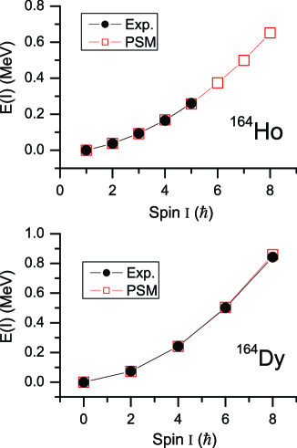
Figure 1: (Color online) Calculated energy levels of the ground band in ¹⁶⁴Ho (upper panel) and ¹⁶⁴Dy (lower panel) are compared with data. The ground state of the odd-odd ¹⁶⁴Ho nucleus has $I^{\pi}=1^{+}$.

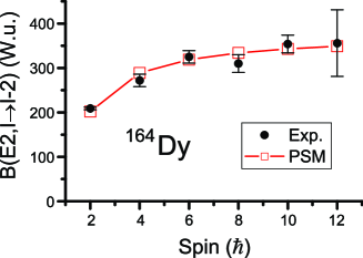
Figure 2: (Color online) Calculated B(E2) values of the ground band in ¹⁶⁴Dy are compared with data.

Under the above calculation conditions, energy levels and wave functions are obtained for the parent ¹⁶⁴Ho and the daughter ¹⁶⁴Dy. In Fig. 1, we compare the calculated energy levels of the ground bands with data. An excellent agreement between theory and experiment is achieved, implying that with this established set of parameters, the structure of these nuclei can be microscopically described. In Fig. 2, one sees that the calculated E2 transition probabilities along the ground band in ¹⁶⁴Dy also agree well with data. These B(E2) values are calculated with the resulting wave functions as

$$B(E2,I_{i}\rightarrow I_{f})={{2I_{f}+1}\over{2I_{i}+1}}\left|\langle\Psi_{I_{f}}||\hat{Q}_{2}||\Psi_{I_{i}}\rangle\right|^{2},$$ (46)

where the effective charges 1.5$e$ for protons and 0.5$e$ for neutrons are used.

IV.2 The Ikeda sum-rule

The above calculations as well as those of the previous PSM publications indicate that for low-lying states in heavy, deformed nuclei, where one has a lot of structure data to compare with, the PSM can usually provide a good description. For GT transitions, a complete description requires the model to cover those highly excited states as well because the GT strength usually spreads for a wide range of excitation and a large amount of GT strength can concentrate in some high energy states. Next, we examine the resulting wave functions of both low-lying and high-lying states in the full model space. There is a well-known charge-exchange sum-rule, the Ikeda sum-rule Ikeda65 , expressed as

$$S(\mathrm{GT^{-}})-S(\mathrm{GT^{+}})$$ (47)

$$= \sum_{f}B(\mathrm{GT^{-}},i\rightarrow f)-\sum_{f}B(\mathrm{GT^{+}},i\rightarrow f)$$

$$= \sum_{f,\mu}|\langle\Psi_{f}|\hat{\beta}^{-}_{1\mu}|\Psi_{i}\rangle|^{2}-\sum_{f,\mu}|\langle\Psi_{f}|\hat{\beta}^{+}_{1\mu}|\Psi_{i}\rangle|^{2}$$

$$= 3(N-Z).$$

This model independent sum-rule results from the commutation relation between the isospin operators. Hence, a (non-relativistic) model is expected to satisfy it as long as the basis in Eq. (47) is complete.

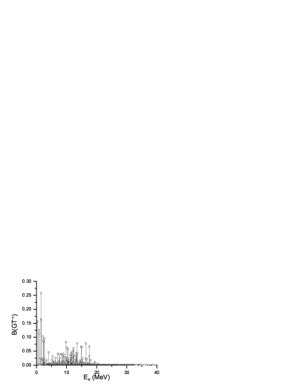
Figure 3: Distribution of the B(GT⁺) strength.

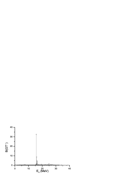
Figure 4: Distribution of the B(GT^-) strength.

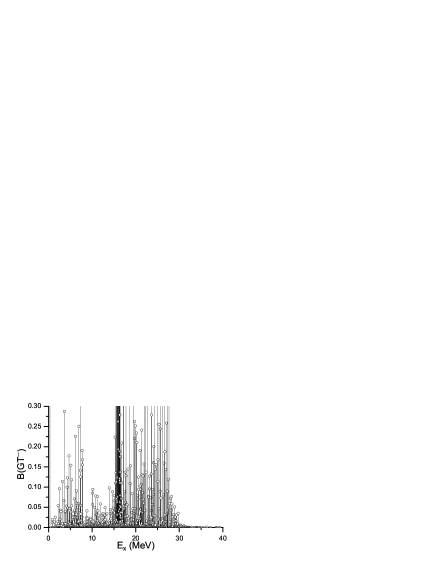
Figure 5: Distribution of the B(GT^-) strength. The numbers are the same as those of Fig. 4, but plotted in the scale as Fig. 3.

Let $|\Psi_{i}\rangle$ in Eq. (47) correspond to the 0-qp ground state of a nucleus and $|\Psi_{f}\rangle$ to the $f$-th 2-qp state with $I^{\pi}=1^{+}$. The summation in Eq. (47) runs over all possible 2-qp $1^{+}$ states in the complete model space. When the single-particle states with $N=$ 3, 4, 5, 6 harmonic-oscillator shells are taken into account for both neutrons and protons, the total number of $1^{+}$ states turns out to be 1718. For our example of ¹⁶⁴Dy ($N=98$ and $Z=66$), we show in Figs. 3, 4, and 5 all the obtained B(GT⁺) and B(GT^-) strengths as functions of the $1^{+}$ state energy. In Fig. 3, it is observed that a considerable portion of the B(GT⁺) strength appears at the low excitation region less than 2.5 MeV. The rest of the strength is fragmented over many states extended to about 20 MeV. The fragmentation is clearly caused by the residual interactions. In Fig. 4, a strong peak of the B(GT^-) strength appears around 16 MeV, while the rest of the strength spreads for nearly the entire energy region. The concentration around 16 MeV takes most of the B(GT^-) strength, and has a character of GT giant resonance. In Fig. 5, we show the same B(GT^-) distribution as that of Fig. 4, but with a different scale to emphasize those smaller strengths. It is seen that the fragmentation extends to the excitation of 30 MeV.

Adding respectively all the B(GT⁺) and B(GT^-) strengths together, as indicated in Eq. (47), we get

$$S(\mathrm{GT^{-}})=97.4957,~{}~{}~{}~{}S(\mathrm{GT^{+}})=4.1717.$$

This means that our $S(\mathrm{GT^{-}})-S(\mathrm{GT^{+}})$ exhausts 97.2$\%$ of the sum-rule value $3(N-Z)$. Note that in our Nilsson calculation for deformed single particle states, we use the standard formalism Nilsson69 in which the neutron harmonic-oscillator frequency $\omega_{\nu}$ differs from the proton frequency $\omega_{\pi}$ for $N\neq Z$ nuclei. If we set $\omega_{\nu}=\omega_{\pi}$, the calculated values become

$$S(\mathrm{GT^{-}})=97.7118,~{}~{}~{}~{}S(\mathrm{GT^{+}})=1.7797,$$

which approaches 99.9$\%$ of the sum-rule value. If we further switch off all the pairing interactions, i.e. if we abandon the quasiparticle picture and go back to the particle picture, we get

$$S(\mathrm{GT^{-}})=96.7480,~{}~{}~{}~{}S(\mathrm{GT^{+}})=0.7480.$$

Thus, in the idealized (but not realistic) case in which neutrons and protons move in the same harmonic-oscillator potential well with no pairing interaction, the Ikeda sum-rule (47) is fulfilled exactly. The above results may be taken as an additional nontrivial check for the coding since in all these calculations, the wave functions in Eq. (47) have a form of Eq. (2) and the B(GT) values are computed in a sophisticated way as presented in Sections II and III.

IV.3 Effects of the Gamow-Teller forces and configuration mixing

The GT interaction in Eq. (9) is a new addition to the PSM Hamiltonian (6). The results in Figs. 1 and 2 seem to indicate that the GT forces do not have effects on the low-lying states since with or without the GT forces, the energy levels and electromagnetic transitions are described equally well. The purpose of this section is to study how the new addition of the GT forces influences the B(GT) values and in what extent the configuration mixing modifies the results.

Table 1: Five different cases of the GT transition calculation. In the table, “even-even” means the $0^{+}$ ground state of ¹⁶⁴Dy and “odd-odd” means the $1^{+}$ ground state of ¹⁶⁴Ho. $H_{GT}$ stands for the Gamow-Teller forces in the Hamiltonian.

Case	Even-even		Odd-odd		$H_{GT}$
1	$\{|0\rangle\}$	(1)	$\{\nu[523]{5\over 2}\times\pi[523]{7\over 2}\}$	(1)	no
2	$\{|0\rangle,|2\nu 2\pi\rangle\}$	(857)	$\{|1\nu 1\pi\rangle\}$	(823)	no
3	$\{|0\rangle\}$	(1)	$\{|1\nu 1\pi\rangle\}$	(823)	yes
4	$\{|0\rangle,|2\nu 2\pi\rangle\}$	(322)	$\{|1\nu 1\pi\rangle\}$	(823)	yes
5	$\{|0\rangle,|2\nu 2\pi\rangle\}$	(857)	$\{|1\nu 1\pi\rangle\}$	(823)	yes

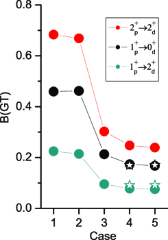
Figure 6: (Color online) B(GT) values calculated for the five different cases. Available data are shown in stars. The B(GT) data are converted from the experimental Log$ft$ values Data through Eq. (45).

We perform calculations for the GT transition from the $1^{+}$ ground state of ¹⁶⁴Ho to the $0^{+}$ ground state of ¹⁶⁴Dy with five different cases as listed in Table I, and results are shown in Fig. 6. For Cases 1 and 2, we do not include the GT forces. In Case 1, there is only one dimension in both the parent ¹⁶⁴Ho and the daughter ¹⁶⁴Dy wave function; namely, we approach the wave function of the even-even nucleus using the projected vacuum state and that of the odd-odd nucleus using the projected 2-qp state $\{\nu[523]{5\over 2}\times\pi[523]{7\over 2}\}$. In Case 2, we include 823 2-qp basis states in the odd-odd and additional 856 4-qp states in the even-even wave function. As one can see from Fig. 6, there is no much difference between Case 1 and Case 2, implying that without the GT forces, configuration mixing becomes unimportant. It is also seen in these two cases that without the GT forces, the calculated B(GT) is by nearly a factor of three too large when compared with data.

A significant reduction in B(GT) is obtained when we switch on the GT forces. As shown in Fig. 6 for Cases 3, 4, and 5, these forces push down the B(GT) values considerably. Moreover, effect of configuration mixing shows up when the GT forces are included; there is a clear difference between the results of Case 3 (with no 4-qp state in the even-even wave function) and Case 4 (with 321 4-qp basis states mixed in the even-even wave function). The latter case reproduces data well. Comparing the result of Case 5 with Case 4, one sees a converging trend in the calculation; further enlarging the configuration space would no longer improve the result as far as the GT transition between the ground states is concerned.

Table 2: Comparison of calculated Log$ft$ values with data for electron-capture from ¹⁶⁴Ho to ¹⁶⁴Dy and $\beta^{-}$ decay from ¹⁶⁴Ho to ¹⁶⁴Er. Data are taken from Ref. Data .

Decay	Log$ft$ (Th.)	Log$ft$ (Exp.)
164Ho ($1^{+}$) $\rightarrow$ 164Dy ($0^{+}$)	4.61	4.59 (8)
164Ho ($1^{+}$) $\rightarrow$ 164Dy ($2^{+}$)	4.96	4.86 (6)
164Ho ($1^{+}$) $\rightarrow$ 164Er ($0^{+}$)	5.19	5.54 (10)
164Ho ($1^{+}$) $\rightarrow$ 164Er ($2^{+}$)	5.62	5.75 (10)

¹⁶⁴Ho can capture an electron and change to ¹⁶⁴Dy, and can $\beta^{-}$-decay to ¹⁶⁴Er. In Table II, we compare calculated Log$ft$ values with the existing data for both processes. We have used the same parameters in generating the ¹⁶⁴Er wave functions and in the calculation of the transition matrix elements. As can be seen from Table II, the agreement in both processes is satisfactory.

IV.4 GT transition rates of the excited states

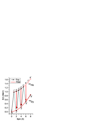
Figure 7: (Color online) Possible transition paths from the ground band of ¹⁶⁴Ho to that of ¹⁶⁴Dy. Experimentally known energies for these states are also displayed.

In Fig. 7, possible allowed GT transitions from the ground band of ¹⁶⁴Ho to that of ¹⁶⁴Dy are illustrated. Here, energy levels up to about 800 keV of excitation in both parent and daughter nuclei are considered. They are $\Delta I=I_{p}-I_{d}=+1$ transitions (in black), $\Delta I=0$ transitions (in red), and $\Delta I=-1$ transitions (in green). The calculated B(GT) values are shown in the upper panel, and the corresponding Log$ft$ values in the lower panel of Fig. 8. The experimentally measured decay probabilities are those of the $I_{p}=1\rightarrow I_{d}=0$ and $I_{p}=1\rightarrow I_{d}=2$ transitions, with which our calculation agrees well. The other transition probabilities associated with the excited states are our prediction. Note that the decay rates with $\Delta I=0$ (in red) are predicted to have larger B(GT) and smaller Log$ft$ values than the measured $\Delta I=\pm 1$ transitions. This is an interesting result because normally, it is very difficult to study $\beta$-decay rates of excited states in laboratory since excited nuclear states decay much faster via $\gamma$-emission than by $\beta$-decay. A measurement may be possible only if the underlying states are long-lived isomers.

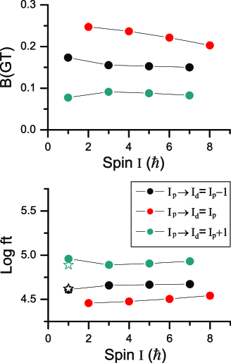
Figure 8: (Color online) Calculated B(GT) (upper panel) and Log$ft$ values (lower panel) for the ¹⁶⁴Ho $\rightarrow$ ¹⁶⁴Dy electron-capture process. Available data are shown in stars. Data are taken from Ref. Data .

In stellar environments, nuclei that are exposed to high temperatures and high densities may experience a significant enhancement in their decay rate. This idea was brought out early by Cameron Cameron59 and studied in detail by Bahcall Bahcall61 . The enhancement can result from the effects related to the thermal population of excited nuclear states in the hot photon bath. In a thermal equilibrium with temperature $T$, the population probability is determined by the Boltzmann factor and the statistical weight

$$p_{i}={{(2I_{i}+1)e^{-E_{i}/kT}}\over{\sum_{m}(2I_{m}+1)e^{-E_{m}/kT}}}.$$ (48)

Hence the actual stellar decay rate must consider decays of all thermally populated excited states $i$ in the parent nucleus to the accessible levels $j$ of the daughter. Thermal enhancement of beta-decay rates can have substantial impact on nucleosynthesis, for example, the s-process branching conditions Kaeppeler99 .

V Summary and outlook

In this article, we have presented the new development of a shell model method for calculation of Gamow-Teller transition rates. The method is based on the Projected Shell Model. Different from the conventional shell model, which builds its states in a spherical basis, the PSM constructs its states in a deformed basis in which important nuclear correlations are taken into account very efficiently. Therefore, it is possible for a shell model diagonalization in the PSM to be carried out in a manageable space for medium to heavy, and even for super-heavy nuclei.

We have shown how the GT transition matrix elements are calculated in the PSM framework. A computer code has been developed and been tested. One nontrivial test has been done through the Ikeda sum-rule. We have obtained a reasonable distribution of the B(GT) strength with a fulfillment of the sum-rule. We have presented the first example from the rare earth region. In the calculation of ¹⁶⁴Ho $\rightarrow$ ¹⁶⁴Dy electron-capture process, we have predicted the GT transition rates for the excited states. Such rates should be included as part of the total rate when these states are thermally populated in hot stellar environments.

In the calculation discussed so far, we have considered only allowed $\beta$-decay for the low-lying states. Calculation of allowed $\beta$-decay for states with high excitation and the forbidden transitions is possible in the PSM framework. Study of GT giant resonance is also under consideration.

The method described in the present article can be applied to various fields such as nuclear astrophysics and fundamental physics, where weak interaction processes take place in nuclear systems ALW05 . In particular, one may find interesting applications to cases where a laboratory measurement for certain weak interaction rates is difficult and where the conventional shell model calculations are not feasible. Potential applications in nuclear astrophysics are calculations of $\beta$-decay rates for the r-process r-process and the rp-process rp-process nucleosynthesis, and electron-capture rates for the core collapse supernova modelling LM03 ; SN . In the double-$\beta$ decay theory, theoretical calculations for the nuclear matrix elements are needed, for which one has relied on the Quasiparticle Random Phase Approximation Civitarese98 ; double-beta , particularly when heavy nuclei are involved. We expect that the method presented here can make important contributions to all these studies.

VI Acknowledgement

The authors are grateful to the Joint Institute for Nuclear Astrophysics (JINA) for support. Z.-C. G. thanks H. Schatz and M. Wiescher for the warm hospitality. Y.S. thanks J. Hirsch for many suggestive discussions. Comments and suggestions from A. Arima, B. A. Brown, J. Engel, and V. Zelevinsky are acknowledged. This work is partly supported by NNSF of China under contract No. 10305019, 10475115, 10435010, by MSBRDP of China (G20000774), and by NSF of USA under contract PHY-0140324 and PHY-0216783.

References

- [1] G. M. Fuller, W. A. Fowler, and M. J. Newman, Ap. J. Suppl. 42, 447 (1980).
- [2] G. M. Fuller, W. A. Fowler, and M. J. Newman, Ap. J. 252, 715 (1982).
- [3] G. M. Fuller, W. A. Fowler, and M. J. Newman, Ap. J. Suppl. 48, 279 (1982).
- [4] G. M. Fuller, W. A. Fowler, and M. J. Newman, Ap. J. 293, 1 (1985).
- [5] M. B. Aufderheide, S. D. Bloom, D. A. Resler, and G. J. Mathews, Phys. Rev. C 47, 2961 (1993).
- [6] K. Langanke and G. Martínez-Pinedo, Rev. Mod. Phys. 75, 819 (2003).
- [7] B. H. Wildenthal, Prog. Part. Nucl. Phys. 11, 5 (1984).
- [8] B. A. Brown and B. H. Wildenthal, At. Data Nucl. Data Tables 33, 347 (1985).
- [9] T. Oda, M. Hino, K. Muto, M. Takahara, and K. Sato, At. Data Nucl. Data Tables 56, 231 (1994).
- [10] E. Caurier, A. P. Zuker, A. Poves, G. Martínez-Pinedo, Phys. Rev. C 50, 225 (1994).
- [11] K. Langanke and G. Martínez-Pinedo, At. Data Nucl. Data Tables 79, 1 (2001).
- [12] K. Hara and Y. Sun, Int. J. Mod. Phys. E 4, 637 (1995).
- [13] J. A. Sheikh and K. Hara, Phys. Rev. Lett. 82, 3968 (1999).
- [14] Y. S. Chen and Z. C. Gao, Phys. Rev. C 63, 014314 (2001).
- [15] Y. Sun, C.-L. Wu, K. Bhatt and M. Guidry, Nucl. Phys. A 703, 130 (2002).
- [16] Y. Sun and C.-L. Wu, Phys. Rev. C 68, 024315 (2003).
- [17] Z. C. Gao, Y. S. Chen, and Y. Sun, Phys. Lett. B 634, 195 (2006).
- [18] A. Aprahamian and Y. Sun, Nature Phys. 1, 81 (2005).
- [19] Y. Sun, M. Wiescher, A. Aprahamian, and J. Fisker, Nucl. Phys. A 758, 765 (2005).
- [20] Y. Sun, X.-R. Zhou, G.-L. Long, E.-G. Zhao, and P. M. Walker, Phys. Lett. B 589, 83 (2004).
- [21] P. Ring and P. Schuck, The Nuclear Many Body Problem (Springer-Verlag, New York, 1980).
- [22] A. R. Edmonds, Angular Momentum in Quantum Mechanics (Princeton University Press, Princeton, 1974).
- [23] S. G. Nilsson, C. F. Tsang, A. Sobiczewski, Z. Szymaski, S. Wycech, C. Gustafson, I.-L. Lamm, P. Möller, and B. Nilsson, Nucl. Phys. A 131, 1 (1969).
- [24] V. A. Kuz’min and V. G. Soloviev, Nucl. Phys. A 486, 118 (1988).
- [25] H. Homma, E. Bender, M. Hirsch, K. Muto, H. V. Klapdor-Kleingrothaus, and T. Oda, Phys. Rev. C 54, 2972 (1996).
- [26] J. Suhonen and O. Civitarese, Phys. Rep. 300, 123 (1998).
- [27] O. Moreno, P. Sarriguren, R. Álvarez-Rodríguez, and E. Moya de Guerra, Prog. Part. Nucl. Phys. 57, 254 (2006).
- [28] D. J. Thouless, Nucl. Phys. 21, 225 (1960).
- [29] K. Tanabe, K. Enami and N. Yoshinaga, Phys. Rev. C 59, 2492 (1999).
- [30] A. Bohr and B. R. Mottelson, Nuclear Structure (W.A. Benjamin, Inc., New York, 1975), Vol. II.
- [31] K. Langanke and G. Martínez-Pinedo, Nucl. Phys. A 673, 481 (2000).
- [32] A. K. Jain, R. K. Sheline, P. C. Sood, and K. Jain, Rev. Mod. Phys. 62, 393 (1990).
- [33] K. Ikeda, T. Udagawa, and H. Yamaura, Prog. Theor. Phys. 175, 22 (1965).
- [34] B. Singh, Nucl. Data Sheets 93, 243 (2001).
- [35] A. Cameron, Ap. J. 130, 452 (1959).
- [36] J. Bahcall, Phys. Rev. 124, 495 (1961).
- [37] F. Käppeler, Prog. Part. Nucl. Phys. 43, 419 (1999).
- [38] A. Aprahamian, K. Langanke, and M. Wiescher, Prog. Part. Nucl. Phys. 54, 535 (2005).
- [39] B. Pfeiffer, K.-L. Kratz, F.-K. Thielemann, and W. B. Walters, Nucl. Phys. A 693, 282 (2001).
- [40] H. Schatz, A. Aprahamian, J. Görres, M. Wiescher, T. Rauscher, J. F. Rembges, F.-K. Thielemann, B. Pfeiffer, P. Möller, K.-L. Kratz, H. Herndl, B. A. Brown, and H. Rebel, Phys. Rep. 294, 167 (1998).
- [41] W. R. Hix, O. E. B. Messer, A. Mezzacappa, M. Liebendörfer, J. Sampaio, K. Langanke, D. J. Dean, and G. Martínez-Pinedo, Phys. Rev. Lett. 91, 201102 (2003).
- [42] S. R. Elliott and P. Vogel, Annu. Rev. Nucl. Part. Sci. 52, 115 (2002).