Charge fluctuations and electric mass in a hot meson gas

Abstract

Net-Charge fluctuations in a hadron gas are studied using an effective hadronic interaction. The emphasis of this work is to investigate the corrections of hadronic interactions to the charge fluctuations of a non-interacting resonance gas. Several methods, such as loop, density and virial expansions are employed. The calculations are also extended to $SU(3)$ and some resummation schemes are considered. Although the various corrections are sizable individually, they cancel to a large extent. As a consequence we find that charge fluctuations are rather well described by the free resonance gas.

I Introduction

The study of event-by-event fluctuations or more generally fluctuations and correlations in heavy ion collisions has recently received considerable interest. Fluctuations of multiplicities and their ratios mult_fluct , transverse momentum pt_fluct_na49 ; pt_fluct_ceres ; pt_fluct_star ; pt_fluct_phenix and net charge fluctuations star_q ; na49_q ; phenix_q ; ceres_q have been measured. Also first direct measurements of two particle correlations have been carried out trainor ; phobos .

Conceptually, fluctuations may reveal evidence of possible phase transitions and, more generally, provide information about the response functions of the system Jeon:2003gk . For example, it is expected that near the QCD critical point long range correlation will reveal themselves in enhanced fluctuations of the transverse momentum ($p_{t}$) per particle Stephanov:1999zu . Also, it has been shown that the fluctuations of the net charge are sensitive to the fractional charges of the quarks in the Quark Gluon Plasma (QGP) Jeon:2000wg ; Asakawa:2000wh .

Most fluctuation measures investigated so far are integrated ones, in the sense that they are related to integrals of many particle distributions koch_bialas . Examples are: Multiplicity, charge and momentum fluctuations which are all related to two-particle distributions. These integrated measures have the advantage that they can be related to well defined quantities in a thermal system. For example, fluctuations of the net charge are directly related to the charge susceptibility. However, in an actual experiment additional, dynamical, i.e non-thermal correlations may be present which make a direct comparison with theory rather difficult. This is particularly the case for fluctuations of the transverse momentum, where the appearance of jet like structures provides nontrivial correlations star_back2back ; phenix_back2back ; trainor . These need to be understood and eliminated from the analysis before fluctuation measurements can reveal insight into the matter itself.

In this article we will not be concerned with the comparison with experimental data, and the difficulties associated with it. We rather want to investigate to which extent interactions affect fluctuations. Specifically, we will study the fluctuations of the net electric charge of the system, the so-called charge fluctuations (CF). CF have been proposed as a signature for the formation of the Quark Gluon Plasma (QGP) in heavy ion collisions Asakawa:2000wh ; Jeon:2000wg . Refs. Asakawa:2000wh ; Jeon:2000wg note that CF per degree of freedom should be smaller in a QGP as compared to a hadron gas because the fractional charges of the quarks enter in square in the CF. Using noninteracting hadrons and quarks, gluons, respectively, it was found that the CF per entropy are about a factor of 3 larger in a hadron gas than in a QGP. The net CF per entropy has in the meantime been measured star_q ; na49_q ; phenix_q ; ceres_q . At RHIC energies the data are consistent with the expectations of a hadron gas, but certainly not with that of a QGP. This might be due to limited acceptance as discussed in bleicher ; stephanov ; gale .

The original estimates of the net charge fluctuations per entropy in the hadron gas Asakawa:2000wh ; Jeon:2000wg have been based on a system of noninteracting particles and resonances. While this model has been proven very successful in describing the measured single particle yields redlich ; becattini , it is not obvious to which extent residual interactions among the hadronic states affect fluctuation observables. For example, in the QGP phase, lattice QCD calculations for the charge susceptibility and entropy-density differ from the result for a simple weakly interacting QGP. Their ratio, however, agrees rather well with that of a noninteracting classical gas of quarks and gluons Kapusta:1992fm ; Jeon:2000wg ; Jeon:2003gk ; Allton:2005gk ; Gupta_net_charge . As far as the hadronic phase is concerned, lattice results for charge fluctuations are only available for systems with rather large pion masses Allton:2005gk ; Gupta_net_charge . In this case, an appropriately rescaled hadron gas model seems to describe the lattice results reasonably well redlich_lattice . Lattice calculations with realistic pion masses, however, are not yet available. Thus, one has to rely on hadronic model calculations in order to assess the validity of the noninteracting hadron gas model for the description of CF. In Ref. Eletsky:1993hv the electric screening mass $m_{\rm el}^{2}$ which is closely related to CF has been calculated up to next-to-leading (NLO) order in $\pi\pi$ interaction. However, the fact that thermal loops pick up energies in the resonance region of the $\pi\pi$ amplitude where chiral perturbation theory is no longer valid leads to large theoretical uncertainties.

It is the purpose of this paper to provide a rough estimate of the effect of interactions in the hadronic phase, in particular the effect of the coupling of the $\rho$-meson to the pions. Since $\rho$-mesons are strong resonances which carry the same quantum numbers as the CF this should provide a good estimate for the size of corrections to be expected from a complete calculation; the latter will most likely come from lattice QCD, once numerically feasible.

As a first step we will consider the case of a heavy $\rho$-meson or, correspondingly, a low temperature approximation. In this case the $\rho$-meson is not dynamical and will not be part of the statistical ensemble. It will only induce an interaction among the pions which closely corresponds to the interaction from the lowest order (LO) chiral Lagrangian.

Although the temperatures in the hadronic phase are well below the $\rho$-mass, it is interesting to estimate the residual $\pi\pi$ correlations introduced when this resonance is treated dynamically. Special attention is paid to charge conservation and unitarity. In addition, we will investigate the importance of quantum statistics. Finally an extension to strange degrees of freedom is provided.

This paper is organized as follows. After a brief review of the charge fluctuations we introduce our model Lagrangian and discuss the heavy rho limit. Next we discuss the treatment of dynamical $\rho$-mesons up to two-loop order and compare with the results obtained in the heavy rho limit. Then, the effect of quantum statistics and unitarity is discussed. Before we show our final results including strange degrees of freedom, we will briefly comment on possible resummation schemes.

II Charge fluctuations and Susceptibilities

Before turning to the model interaction employed in this work, let us first introduce some notation and recall the necessary formalism to calculate the CF (for details, see, e.g., Ref. Jeon:2003gk ).

In this work we will consider a system in thermal equilibrium. In this case the charge fluctuations $\left\langle\delta Q^{2}\right\rangle$ are given by the second derivative of the appropriate free energy $F$ with respect to the charge chemical potential $\mu$:

$$\left\langle\delta Q^{2}\right\rangle=-T\frac{\partial^{2}F}{\partial\mu^{2}}=-VT\chi_{Q}.$$ (1)

Here, $T$ ($V$) is the temperature (volume) of the system and $\chi_{Q}$ is the charge susceptibility, which is often the preferred quantity to consider, particularly in the context of lattice QCD calculations. Equivalently, the CF or susceptibility are related to the electromagnetic current-current correlation function Ka1989 ; Prakash:2001xm

$$\Pi_{\mu\nu}(\omega,{\bf k})=\rm i\int dtd^{3}x\,e^{-i(\omega t-{\bf kx})}\left\langle J_{\mu}({\bf x},t)J_{\nu}(0)\right\rangle$$ (2)

via

$$\left\langle\delta Q^{2}\right\rangle=VT\,\Pi_{00}(\omega=0,{\bf k}\rightarrow 0)=VTm_{{\rm el}}^{2}$$ (3)

which is illustrated for scalar QED in Appendix A. Relation (3) also establishes the connection between the CF and the electric screening mass $m_{\rm el}$.

As noted previously, the observable of interest is the ratio of CF over entropy

$$D_{S}\equiv\frac{\left\langle\delta Q^{2}\right\rangle}{e^{2}S}.$$ (4)

Given a model Lagrangian, both CF and entropy can be evaluated using standard methods of thermal field theory (see e.g. Ka1989 ). CF are often evaluated via the current-current correlator using thermal Feynman rules; evaluating the free energy and using relation (1) will lead to the same results as will be demonstrated in Sec. V.

Let us close this section by noting that in an actual experiment a direct measurement of the entropy is rather difficult. However, the number of charged particles $\langle N_{{\rm ch}}\rangle$ in the final state is a reasonable measure of the final state entropy. Therefore, the ratio

$$D_{c}=4\;\frac{\langle\delta Q^{2}\rangle}{e^{2}\langle N_{{\rm ch}}\rangle}.$$ (5)

has been proposed as a possible experimental observable for accessing the CF per degree of freedom. For details and corrections to be considered see Ref. Jeon:2003gk and references therein. In this article we will concentrate on the “theoretical” observable $D_{S}$ defined in Eq. (4).

III Model Lagrangian and $\bm{\pi\pi}$ interaction in the heavy $\bm{\rho}$ limit

As already discussed in the Introduction, in this work we want to provide an estimate of the corrections to the CF introduced by interactions among the hadrons in the hadronic phase. Since it is impossible to account for all hadrons and their interactions, we will concentrate on a system of pions and $\rho$-mesons only, with some extensions to $SU(3)$ in later sections. A suitable effective Lagrangian for this investigation is the “hidden gauge” approach of Refs. Bando:1984ej ; Kaymakcalan:1984bz . In this model the $\rho$-meson is introduced as a massive gauge field. The $\pi\rho$ interaction results from the covariant derivative $D_{\mu}\Phi=\partial_{\mu}\Phi-\frac{ig}{2}\;\left[\rho_{\mu},\Phi\right]$ acting on the pion field $U(x)=\exp[i\Phi(x)/f_{\pi}]$ in the LO chiral Lagrangian

$${\cal L}_{\pi\pi}^{(2)}=\frac{f_{\pi}^{2}}{4}\;{\rm Tr}\left[\partial_{\mu}U^{\dagger}\partial^{\mu}U+{\cal M}(U+U^{\dagger})\right]$$ (6)

by the replacement $\partial_{\mu}\to D_{\mu}$. Here,

$$\Phi=\left(\begin{array}[]{cc}\pi^{0}&\sqrt{2}\pi^{+}\\ \sqrt{2}\pi^{-}&-\pi^{0}\end{array}\right),\quad\rho_{\mu}=\left(\begin{array}[]{cc}\rho_{\mu}^{0}&\sqrt{2}\rho_{\mu}^{+}\\ \sqrt{2}\rho_{\mu}^{-}&-\rho_{\mu}^{0}\end{array}\right)$$ (11)

and $f_{\pi}=93$ MeV is the pion decay constant. An extension of the heavy gauge model to $SU(3)$ has been applied for vacuum and in-medium processes (see, e.g., Refs. Klingl:1996by ; Alvarez-Ruso:2002ib ) and is straightforward Marco:1999df . This extension is considered in Sec. VII.1.

The resulting $\pi\rho$ interaction terms are

$${\cal L}_{\rho\pi\pi}=\frac{ig}{4}\;{\rm Tr}\left(\rho_{\mu}\left[\partial^{\mu}\Phi,\Phi\right]\right)$$ (12)

and

$${\cal L}_{\rho\rho\pi\pi}=-\;\frac{g^{2}}{16}\;{\rm Tr}\left(\left[\rho_{\mu},\Phi\right]^{2}\right).$$ (13)

Chiral corrections to the interaction in Eq. (12) are of ${\cal O}(p^{5})$ or higher as pointed out in Ref. Birse:1996hd . The interaction of Eq. (13) does not depend on the pion momentum, thus violating the low energy theorem of chiral symmetry Birse:1996hd . Nevertheless, this term is required by the gauge invariance of the $\rho$-meson Cabrera:2000dx and in fact cancels contributions in the pole term and crossed pole term of $\pi\rho$ scattering via Eq. (12).

To leading order in the pion field we, thus, have the following model Lagrangian:

$${\cal L}={\cal L}_{\Phi}+{\cal L}_{\rho}+{\cal L}_{\rho\pi\pi}+{\cal L}_{\rho\rho\pi\pi}$$ (14)

with the free field terms

$${\cal L}_{\Phi} = \frac{1}{4}{\rm Tr}\left(\partial_{\mu}\Phi\partial^{\mu}\Phi\right)-\frac{1}{4}{\rm Tr}\left(m_{\pi}^{2}\Phi^{2}\right),$$

$${\cal L}_{\rho} = -\frac{1}{8}\;{\rm Tr}\left(G_{\mu\nu}G^{\mu\nu}\right)+\frac{1}{4}{\rm Tr}\left(m_{\rho}^{2}\rho_{\mu}\rho^{\mu}\right),$$ (15)

and the interaction terms ${\cal L}_{\rho\pi\pi}$ and ${\cal L}_{\rho\rho\pi\pi}$ as given in Eq. (12) and (13), respectively. For the kinetic tensor of the $\rho$, $G_{\mu\nu}=\partial_{\mu}\rho_{\nu}-\partial_{\nu}\rho_{\mu}$, we restrict ourselves to the Abelian part; a non-Abelian $\rho$ would lead to additional $3\rho$ and $4\rho$ couplings. In the thermal loop expansion this would result in closed $\rho$ loops which are kinematically suppressed. The coupling constant $g$ is fixed from the $\rho\rightarrow\pi\pi$ decay to be $g=g_{\rho\pi\pi}=6$ and and we use $m_{\pi}=138$ MeV and $m_{\rho}=770$ MeV throughout this paper.

As a first approximation, we start with the low temperature limit of the $\pi\pi$ interaction in which the $\rho$-meson mediates the interaction of the pions but does not enter the heatbath as an explicit degree of freedom. To this end we construct an effective interaction based on $s$-, $t$-, and $u$-channel $\rho$-meson exchange as given by second order perturbation theory of the interaction ${\cal L}_{\rho\pi\pi}$. Furthermore, we assume that the momentum transfer $k^{2}$ of two pions interacting via a $\rho$ is much smaller than the mass of the $\rho$–meson, $m_{\rho}^{2}>>k^{2}$, i.e. we replace the propagator of the exchanged $\rho$-meson by $-1/m_{\rho}^{2}$. Thus, we arrive at the following effective interaction

$${\cal L}^{{\rm eff}}_{\pi\pi} = \frac{g^{2}}{2m_{\rho}^{2}}\big{(}(\pi^{-}\stackrel{{\scriptstyle\leftrightarrow}}{{\partial_{\mu}}}\pi^{+})^{2}-2(\pi^{0}\stackrel{{\scriptstyle\leftrightarrow}}{{\partial_{\mu}}}\pi^{+})(\pi^{0}\stackrel{{\scriptstyle\leftrightarrow}}{{\partial^{\mu}}}\pi^{-})\big{)}.$$ (16)

Note that in this limit, subsequently referred to as the “heavy $\rho$ limit” the $\rho\rho\pi\pi$ term from Eq. (13) does not contribute at order $g^{2}$.

The effective Lagrangian of Eq. (16) shows the identical isospin and momentum structure as the kinetic term of Eq. (6) at $1/f_{\pi}^{2}$. However, comparing the overall coefficient one arrives at

$$m_{\rho}^{2}=3f_{\pi}^{2}g^{2}$$ (17)

which differs by a factor of $3/2$ from the well known KSFR relation KSFR $m_{\rho}^{2}=2f_{\pi}^{2}g^{2}$. We should point out the same factor has been observed in the context of the anomalous $\gamma\pi\pi\pi$ interaction Cohen:1989es . As discussed in more detail in Appendix B.1 the KSFR relation is recovered if one restricts the model to the $s$-channel diagrams for the isovector $p$-wave ($T_{11}$) amplitude. Once also $t$- and $u$-channels are taken into account the factor $3/2$ appears. For this study, we prefer the interaction (16) over ${\cal L}_{\pi\pi}^{(2)}$ from Eq. (6) as it delivers a better data description at low energies in the $\rho$-channel (see Appendix B.1). The simplification from the ”heavy $\rho$” limit of the $\pi\pi$ interaction will later be relaxed in favor of dynamical $\rho$-exchange. However, the interaction in the heavy $\rho$ limit will still serve as a benchmark for the more complex calculations.

Since we are interested in the electromagnetic polarization tensor, the interaction of Eq. (16), together with the kinetic term of the pion, is gauged with the photon field by minimal substitution, leading to

$${\cal L}_{\pi\gamma} = -\frac{1}{4}\left(F^{\mu\nu}\right)^{2}-m_{\pi}^{2}\big{(}\pi^{+}\pi^{-}+\frac{1}{2}(\pi^{0})^{2}\big{)}+(D_{\mu}^{*}\pi^{-})(D^{\mu}\pi^{+})+\frac{1}{2}\>\left(\partial_{\mu}\pi^{0}\right)^{2},$$ (18)

$$+ \frac{g^{2}}{2m_{\rho}^{2}}\left(\pi^{-}D_{\mu}\pi^{+}-\pi^{+}D_{\mu}^{*}\pi^{-}\right)^{2}-\frac{g^{2}}{m_{\rho}^{2}}\left(\pi^{0}D^{\mu}\pi^{+}-\pi^{+}\partial^{\mu}\pi^{0}\right)\left(\pi^{0}D_{\mu}^{*}\pi^{-}-\pi^{-}\partial_{\mu}\pi^{0}\right)$$

with the covariant derivative of the photon field $D_{\mu}=\partial_{\mu}+ieA_{\mu}$, $e>0$, and the photon field tensor $F^{\mu\nu}$, leading to the $\gamma\pi\pi$ and $\gamma\gamma\pi\pi$ interactions of scalar QED, plus $\gamma\pi\pi\pi\pi$ and $\gamma\gamma\pi\pi\pi\pi$ vertices. Vector meson dominance leads to $\gamma\rho^{0}$ mixing as pointed out, e.g., in Ref. Klingl:1996by , additionally to the vertices of Eq. (18). However, since the correlator of Eq. (3) is evaluated at the photon point, the form factor is unity and the process $\gamma\to\rho^{0}\to\pi\pi$ which emerges in the systematic approach of Ref. Schechter:1986vs does not contribute to the $\gamma\pi\pi$ coupling. Thus, no modification of Eq. (18) is required. Note also that the anomalous interaction providing $\gamma\pi\rho$ vertices Klingl:1996by does not contribute in the long-wavelength limit studied here. This follows a general rule noted in Ref. Kapusta:1992fm .

In the following chapters, the $\rho$ will be also treated dynamically. The interaction with the photon is then given by the scalar QED vertices from above, plus a $\gamma\rho\pi\pi$ vertex which is obtained from Eq. (12) by minimal substitution. With the same procedure the direct $\gamma\rho$ interaction is constructed from Eq. (15), leading to the vertices

$$\includegraphics[width=71.13188pt]{eq_15_1.eps}\;\;{\hat{=}}\;e\left(k^{\nu}g_{\mu\sigma}+k^{\prime\sigma}g_{\mu\nu}-(k+k^{\prime})^{\mu}g_{\sigma\nu}\right),\quad\includegraphics[width=56.9055pt]{eq_15_2.eps}\;\;{\hat{=}}\;2e^{2}\left(g_{\mu\beta}g_{\alpha\nu}-g_{\mu\nu}g_{\alpha\beta}\right)$$ (19)

in the imaginary time formalism.

IV Charge fluctuations at low temperatures

Having introduced the effective interaction in the heavy $\rho$ limit, we can evaluate the correction to the CF due to this interaction. Before discussing the results let us first remind the reader about the basic relations for CF in a noninteracting gas of pions and $\rho$-mesons.

IV.1 Charge fluctuations for free pions and $\rho$-mesons

In order to illustrate the relations of Sec. II and to establish a baseline it is instructive to calculate $D_{S}$ from Eq. (4) for the free pion gas in two ways: once via Eq. (3) and also directly from statistical mechanics. The interaction from Eq. (18) reduces to scalar QED in the zeroth order in $g$. To order $e^{2}$ the selfenergy is given by the set of gauge invariant diagrams in Fig. 1

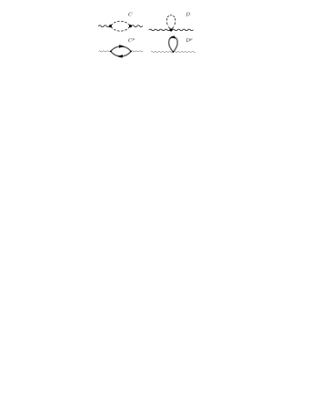
Figure 1: Photon selfenergy at $e^{2}$ for the free pion gas ($C,\,D$) and the free $\rho$ gas ($C^{\rho},\,D^{\rho}$).

and reads

$$\Pi^{00}(k^{0}=0,{\bf k\to 0})=e^{2}\left(C+D\right),\quad\left\langle\delta Q^{2}\right\rangle=e^{2}TV\left(C+D\right)$$ (20)

according to Eq. (3) with

$$C=\frac{1}{\pi^{2}}\int\limits_{0}^{\infty}dp\;\omega\;n[\omega],\quad D=\frac{1}{\pi^{2}}\int\limits_{0}^{\infty}dp\;p^{2}\;\frac{n[\omega]}{\omega}$$ (21)

where $\omega=\sqrt{p^{2}+m_{\pi}^{2}}$ the pion energy, $n[\omega]=1/(\exp\left(\beta\omega\right)-1)$ the Bose-Einstein factor, and $\beta=1/T$. The CF from Eq. (20) can also be derived from statistical mechanics,

$$\left\langle\delta Q^{2}\right\rangle=e^{2}T^{2}\;\frac{\partial^{2}}{\partial\mu^{2}}|_{\mu=0}\log Z,$$ (22)

$$\log Z_{0}(\mu)=-V\int\frac{d^{3}p}{\left(2\pi\right)^{3}}\;\sum_{\mu_{i}=\pm\mu,0}\log\left(1-e^{-\beta(\omega+\mu_{i})}\right).$$ (23)

Both the photon selfenergy and Eq. (22) lead to the same CF also at the perturbative level as will be seen in Sec. V. The value for the chemical potential of $\mu_{i}=\pm\mu$ in Eq. (23) corresponds to charged pions and $\mu_{i}=0$ is assigned to neutral pions which do not contribute to the CF but to the entropy $S=\partial(T\log Z)/\partial T$ of the free gas,

$$S_{0}=\frac{1}{2\pi^{2}}\;\frac{V}{T}\;\int\limits_{0}^{\infty}dp\;p^{2}\;n[\omega]\left(3\omega+\frac{p^{2}}{\omega}\right).$$ (24)

In the high temperature limit, or for massless pions, the relevant thermodynamical quantities are given by

$$\left\langle\delta Q^{2}\right\rangle=\frac{e^{2}V}{3}T^{3},\quad S=\frac{2\pi^{2}V}{15}T^{3},\quad\langle N_{\rm ch}\rangle=\frac{2\zeta(3)V}{\pi^{2}}T^{3}$$ (25)

where $\langle N_{\rm ch}\rangle$ is defined as in Ref. Jeon:2000wg . For the quantity $D_{S}$ from Eq. (4) we obtain $D_{S}=0.185$ for massive free pions at $T=170$ MeV and $D_{S}=0.253$ for massless pions. For $D_{c}$ from Eq. (5), the values are $4.52$ and $5.47$, respectively.

The classical (Boltzmann) limit is obtained by replacing the Bose-Einstein distribution $n$ in Eqs. (21) and (24) by the Boltzmann distribution $n_{\rm B}=\exp(-\beta\omega)$. In this case at $T=170$ MeV we obtain $D_{S}=0.156$ and $D_{S}=1/6$ for massive and massless pions, respectively. For all masses and temperatures, $D_{c}=4$ the classical limit. For a QGP made out of massless quarks and gluons, $D_{S}=0.034$, following the same arguments as in Jeon:2000wg . This is about a factor of five smaller than a pion gas.

The CF for the free $\rho$ gas are given by the diagrams with the double lines in Fig. 1. With the $\rho$ propagator

$$D^{\mu\nu}=\frac{1}{k^{2}-m_{\rho}^{2}+i\epsilon}\left(g^{\mu\nu}-\frac{k^{\mu}k^{\nu}}{m_{\rho}^{2}}\right)$$ (26)

and the interaction from Eq. (19) the photon selfenergy turns out to be

$$\Pi_{\rho}^{00}(k^{0}=0,{\bf k\to 0})=3e^{2}[C^{\rho}+D^{\rho}]$$ (27)

where the upper index means that the pion mass is substituted by the $\rho$-mass in $C$ and $D$ from Eq. (21). The factor of three corresponds to the sum over the physical polarizations of the $\rho$. The same factor also appears in $\log Z_{0}$ of Eq. (23) for the $\rho$.

IV.2 $\bm{\pi\pi}$ interaction in the heavy $\bm{\rho}$ limit to order $\bm{e^{2}g^{2}}$

At order $e^{2}g^{2}$ the Feynman rules derived from the heavy $\rho$ limit Eq. (18) lead to the set of five diagrams (eff1) to (eff5) depicted in Fig. 2. They are gauge invariant as shown in Appendix C.4.

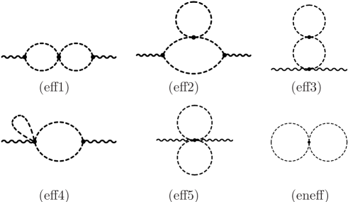
Figure 2: Selfenergy for $\pi\pi$ interaction in the heavy $\rho$ limit at order $e^{2}g^{2}$ (diagrams (eff1) to (eff5)). Expansion of $\log Z$ at $g^{2}$ for the calculation of the entropy (diagram (eneff)).

The summation over Matsubara frequencies has been performed by a transformation into contour integrals following Ref. Ka1989 . The limit $\displaystyle{(k^{0}=0,{\bf k}\rightarrow{\bf 0})}$ for the external photon has to be taken before summation and integration, as discussed in Appendix A. The loop momenta factorize so that the diagrams of Fig. 2 can be expressed in terms of the quantities $C$ and $D$ from Eq. (21) as shown in Tab. 1.

Table 1: Static selfenergy $\Pi^{00}(k^{0}=0,{\bf k\to 0})$ from Fig. 2 with $C$ and $D$ from Eq. (21).

Diagram	Contribution
(eff1)	$\displaystyle{-\frac{3}{2}\frac{e^{2}g^{2}}{m_{\rho}^{2}}\;C^{2}}$
(eff2)	$\displaystyle{-\frac{e^{2}g^{2}}{m_{\rho}^{2}}\;D\big{(}D-3C-\beta\;\frac{\partial}{\partial\beta}\;(C-D)\big{)}}$
(eff3)	$\displaystyle{+\frac{e^{2}g^{2}}{m_{\rho}^{2}}\;D(2D-C)}$
(eff4)	$\displaystyle{-5\frac{e^{2}g^{2}}{m_{\rho}^{2}}\;CD}$
(eff5)	$\displaystyle{-\frac{5}{2}\frac{e^{2}g^{2}}{m_{\rho}^{2}}\;D^{2}}$

The sum of the diagrams is cast in a surprisingly simple form,

$$\sum_{i=1}^{5}\Pi_{i}(k^{0}=0,{\bf k}\to{\bf 0})=-\frac{e^{2}g^{2}}{m_{\rho}^{2}}\left[\frac{3}{2}\left(C+D\right)^{2}-\beta\;D\;\frac{\partial}{\partial\beta}\left(C-D\right)\right].$$ (28)

The entropy correction at $g^{2}$ is calculated from $\log Z$ given by diagram (eneff) in Fig. 2,

$$S_{1}=-\frac{3g^{2}V}{2T}\;\left(\frac{m_{\pi}}{m_{\rho}}\right)^{2}\;D\left(C+D\right).$$ (29)

Note that using the LO chiral Lagrangian from Eq. (6) instead of the $\pi\pi$ interaction in the heavy $\rho$ limit, results would simply change by a factor of $(2/3)^{2}$, up to tiny corrections, which are due to higher order contributions involving the chiral symmetry breaking term $\sim{\cal M}$ from Eq. (6). Numerical results can be found in Sec. VI.2, which supersede our findings from Ref. Doring:2002qa .

V The $\bm{\rho}$–meson in the heatbath

In this section we will relax the assumption of a heavy non-dynamical $\rho$-meson. This will allow for an estimate of the CF from the residual interactions of the $\rho$ when this particle is treated as an explicit degree of freedom. It will also avoid some problems induced in the calculation from vertices of higher order in momenta such as encountered in the ${\cal L}_{\pi\pi}^{(4)}$ calculation in Ref. Eletsky:1993hv (see discussion in Sec. VI.1, VI.2). The $\rho\pi\pi$ interaction from Eq. (12) involves vertices only linear in momentum and a smoother temperature dependence is expected.

We start with the calculation of the diagrams in the first two columns of Fig. 3

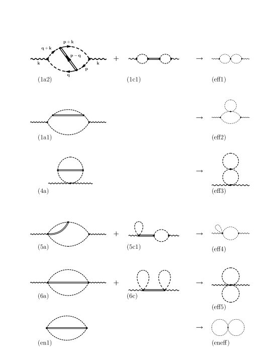
Figure 3: Overview of the relevant two-loop diagrams at $e^{2}g^{2}$ for the photon selfenergy and at $g^{2}$ for the entropy. Diagram (1a2) is calculated in detail in Appendix C, where also the results for all other diagrams and a proof of gauge invariance are found. The diagrams on the right hand side (eff1-eff5) correspond to the heavy $\rho$ limit of the ones given on the left. This limit, indicated with arrows, is numerically shown in Appendix C.1.

because this subset corresponds to the heavy $\rho$ limit from Sec. III; by increasing the $\rho$-mass from its physical value to infinity in these diagrams, the previous results from Tab. 1 are recovered as illustrated in Appendix C.1. Note that there is no need to include $\gamma\rho^{0}$ mixing or anomalous vertices as we have already seen in Sec. III.

Here and in the following sections, the $\rho$ is treated as a stable particle (propagator from Eq. (26)) and we ignore imaginary parts at the cost of unitarity violations as will be discussed in Sec. VI.1. A $\rho$ with finite width would induce problems concerning gauge invariance: one would have to couple the photon to all intermediate $\rho$ selfenergy diagrams that build up the $\rho$ width in the Dyson-Schwinger summation. In principle, this is possible — see the last part of Sec. VIII — but goes beyond the scope of this work. The results for the diagrams with dynamical $\rho$ from Fig. 3 are found in Eq. (58,60) and Fig. 16 of Appendix C.1, together with a detailed calculation of one of the diagrams and a discussion of the infrared divergences. In Appendix C.4 the gauge invariance of the diagrams is shown.

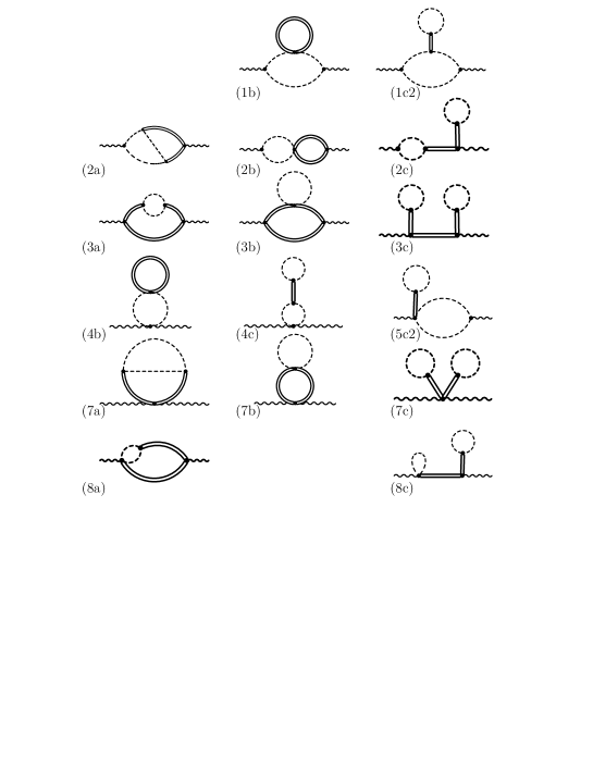
Figure 4: Additional, sub-leading, diagrams at $e^{2}g^{2}$ with direct $(\gamma)\gamma\rho\rho$ couplings and with $\rho\rho\pi\pi$ interaction. Also, the diagrams which vanish are shown [(1c2), (2c), (3c), (4c), (5c2), (7c), (8c)].

At order $e^{2}g^{2}$ there are additional diagrams with direct $\gamma\rho\rho$ and $\gamma\gamma\rho\rho$ couplings from Eq. (19) and also with the $\rho\rho\pi\pi$ coupling from Eq. (13) which is required by the gauge invariance of the $\rho$-meson. The resulting diagrams are displayed in Fig. 4. Some of these diagrams contain more than one $\rho$-propagator. They are sub-dominant because every $\rho$ propagator counts as $1/m_{\rho}^{2}$. Furthermore, Fig. 4 shows diagrams which have a closed pion loop with only one vertex of the $\rho\pi\pi$ type (see, e.g., diagram (2c)). The latter diagrams vanish due to the odd integrand in the loop integration. The set of diagrams from Figs. 3 and 4 is complete at order $e^{2}g^{2}$.

The non-vanishing diagrams from Fig. 4 are best calculated by evaluating the corresponding partition function, $\log Z$, at finite chemical potential $\mu$ and differentiating with respect to $\mu$ Kapusta:1992fm ; Eletsky:1993hv (see also Eq. (22)). For a calculation at finite $\mu$ we first convince ourselves that for the simple interaction from Eq. (16) the use of Eq. (22) leads to the same results as in Sec. IV.2. The calculation at finite $\mu$ implies a shift in the zero-momenta of the propagators and derivative vertices, $p^{0}\to p^{0}\pm\mu$ Eletsky:1993hv ; Ka1989 , depending on the charge states of the particles. The correction to $\log Z(\mu)$ from diagram (a) in Fig. 5

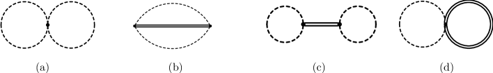
Figure 5: Correction to $\log Z(\mu)$. Diagram (a) shows the $\pi\pi$ interaction in the heavy $\rho$ limit, diagrams (b)–(d) the interaction via explicit vector meson from Eqs. (12) and (13).

with the interaction from Eq. (16) is given by

$$\log Z_{{\rm(a)}}(\mu)=\frac{-g^{2}}{16\;m_{\rho}^{2}}\;\beta V\left[3\left(V_{+}-V_{-}\right)^{2}+m_{\pi}^{2}\left(U_{+}+U_{-}\right)\left(4D+U_{+}+U_{-}\right)\right]$$ (30)

with

$$U_{\pm}=\frac{1}{\pi^{2}}\int\limits_{0}^{\infty}dk\;\frac{k^{2}}{\omega}\;n[w\pm\mu],\quad V_{\pm}=\frac{1}{\pi^{2}}\int\limits_{0}^{\infty}dk\;k^{2}\;n[w\pm\mu]$$ (31)

and $D$ from Eq. (21). Applying Eq. (22) to $\log Z_{{\rm(a)}}(\mu)$ reproduces the result for the photon selfenergy in the heavy $\rho$ limit from Eq. (28) which is shown to be gauge invariant in Appendix C.4.

Thus having established that equivalence of photon selfenergy and charge fluctuations (Eq. (3)) holds on the perturbative level, we are encouraged to evaluate the diagrams of Fig. 4 by differentiating the appropriate terms in $\log Z$ with respect to the chemical potential. The diagrams for $\log Z$ corresponding to the photon self energies given in Figs. 3 and 4 are displayed in Fig. 5(b,c,d). (Details can be found in Appendix C.3).

In Fig. 6 corrections to the electric mass of a free pion gas due to different sets of diagrams are shown. As a reference, we also plot the results for gases of noninteracting pions and noninteracting $\rho$-mesons (”free $\pi$” and ”free $\rho$”).

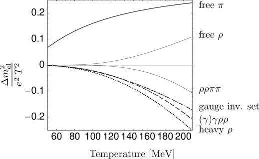
Figure 6: Corrections to $m_{\rm el}$ or CF. Dashed-dotted line: result from the gauge invariant subset of diagrams from the first two columns of Fig. 3. Dashed line: Result from diagrams (b)+(c) from Fig. 5. Dotted line: heavy $\rho$ limit from Sec. IV.2. Solid lines: free $\pi$ gas, free $\rho$ gas, and the $\rho\rho\pi\pi$ interaction from Fig. 5 (d).

The electric mass from the diagrams of Fig. 2 with the $\pi\pi$ interaction in the heavy $\rho$ limit is plotted as the dotted line. The electric mass from the diagrams in the first two columns of Fig. 3 with dynamical $\rho$ is plotted as the dashed-dotted line. At low temperatures, both results coincide (in detail this is also plotted in Fig. 16). However, at higher temperatures we observe significant differences which shows, thus, that the $\rho$ obtains importance as an explicit degree of freedom.

The diagrams (b) and (c) from Fig. 5 correspond to the first two columns of Fig. 3. Additionally, they provide photon selfenergies with $\gamma\rho\rho$ and $\gamma\gamma\rho\rho$ vertices from Fig. 4, diagrams (2a), (3a), (7a), and (8a). As shown in Fig. 6 (dashed line), these additional $\gamma\rho$ couplings obtain some minor influence above $T\sim 150$ MeV.

Additionally, in Fig. 4 there are diagrams with $\rho\rho\pi\pi$ couplings from Eq. (13). The diagrams (1b), (2b), (3b), (4b), and (7b) correspond to diagram (d) in Fig. 5. In the heavy $\rho$ limit these diagrams do not contribute. However, for dynamical $\rho$-mesons these diagrams contribute significantly due to the sum over the spin of the $\rho$. In Fig. 6 the resulting electric mass is displayed as the solid line (”$\rho\rho\pi\pi$”).

VI Relativistic virial expansion

In Ref. Eletsky:1993hv the electric mass has been determined using chiral $\pi\pi$ interaction and thermal loops leading to results that show large discrepancies to a virial calculation of $m_{\rm el}^{2}$. Before we discuss these differences in Sec. VI.1, VI.2 let us review the theoretical framework first. The virial expansion is an expansion of thermodynamic quantities in powers of the fugacities $e^{\beta\mu}$, while the interaction enters as experimentally measured phase-shifts. Consequently, all orders of the interaction are taken into account. Thermal loops, on the other hand, respect quantum statistics (Bose-Einstein in our case) and, thus, contain an infinite subclass of the virial expansion. However, the interaction only enters up to a given order. Thus, the loop and virial expansion represent quite different approximations and it will depend on the problem at hand which is the more appropriate one. The effect on quantum statistics can be considerable. For example at $T=170$ MeV the values for the electric mass $m_{\rm el}^{2}$ of the free $\pi$ gas or the two-loop diagrams, Eq. (28), change by 20% and 38% (!) respectively, if we take the Boltzmann limit. Therefore, it is desirable to have a density expansion that respects particle statistics as well as sums all orders of the interaction. While this might be very difficult if not impossible to do in general, it can be done up to second order in the (Bose-Einstein) density.

The partition function can separated into a free and an interacting part,

$$\log Z=\log Z_{0}+\sum_{i_{1},i_{2}}z_{1}^{i_{1}}\,z_{2}^{i_{2}}\,b(i_{1},i_{2})$$ (32)

in an expansion in terms of the chemical potential $\mu$ with $z_{j}=\exp(\beta\mu_{j})$ for $j=1,2$ the fugacities. In the $S$-matrix formulation of statistical mechanics from Ref. Dashen the second virial coefficient $b(i_{1},i_{2})$ can be separated into a statistical part and a kinematic part containing the vacuum $S$-matrix according to

$$b(i_{1},i_{2})=\frac{V}{4\pi i}\int\frac{d^{3}{\bf k}}{(2\pi)^{3}}\int dE\;e^{-\beta\sqrt{{\bf k}^{2}+E^{2}}}\;{\rm Tr}_{i_{1},i_{2}}\left[AS^{-1}(E)\;\frac{\stackrel{{\scriptstyle\leftrightarrow}}{{\partial}}}{\partial E}\;S(E)\right]_{c}$$ (33)

where $A$ is the (anti)symmetrization operator for interacting (fermions) bosons and the trace is over the sum of connected diagrams (index ”$c$”). In Eq. (33), $V$ is the Volume, $k$ is the momentum of the $n$-particle cluster in the gas rest frame and $E=s^{1/2}$ stands for the total c.m. energy. The labels $i_{1},i_{2}$ indicate a channel of the $S$-matrix with $i_{1}+i_{2}$ particles in the initial state. For the second virial coefficient, $i_{1}=i_{2}=1$.

For $\pi\pi$ scattering, Eq. (33) can be integrated over $k$ and the $S$-matrix can be expressed via phase shifts, weighted with their degeneracy Eletsky:1993hv . With $B_{2}=b(i_{1},i_{2})/V$ in the limit $V\to\infty$ one obtains

$$B_{2}^{(\pi\pi),\;{\rm Boltz}}(\mu=0) = \frac{1}{2\pi^{3}\beta}\;\int\limits_{2m_{\pi}}^{\infty}dE\;E^{2}\;K_{2}(\beta E)\sum_{\ell,I}(2I+1)(2\ell+1)\;\frac{\partial\delta_{\ell}^{I}(E)}{\partial E}$$ (34)

$$= \frac{1}{2\pi^{3}}\;\int\limits_{2m_{\pi}}^{\infty}dE\;E^{2}\;K_{1}(\beta E)\sum_{\ell,I}(2I+1)(2\ell+1)\;\delta_{\ell}^{I}$$

where the second line has been obtained after integration by parts (assuming $\delta_{\ell}^{I}\rightarrow 0$ as $E\rightarrow 2m_{\pi}$). The sum over phase shifts $\delta_{\ell}^{I}$ (isospin $I$, angular momentum $\ell$) is restricted to $\ell+I=$ even and $K_{i}$ are the modified Bessel functions of the second kind. The virial expansion in this or similar form has been applied in numerous studies of the thermal properties of interacting hadrons as, e.g., Welke:1990za ; Venugopalan:1992hy , among them the electric mass Eletsky:1993hv . Note that, e.g. in Eletsky:1993hv , Bose-Einstein statistics is taken into account for the non-interacting, free gas, part. However, it is also possible to include particle statistics for the interacting part. This means the summation of so-called exchange diagrams as outlined in Ref. Dashen , Sec. VIIB. We employ this idea and also include a finite chemical potential. This is achieved by projecting the binary collisions of pions in different charge states to the isospin channels Eletsky:1993hv . Additionally, the interaction $T$ matrix is boosted from the gas rest frame to the two-particle c.m. frame and the $T$-matrix is defined via phase shifts with the final result

$$B_{2}^{(\pi\pi),\;{\rm Bose}}(\mu) = \frac{\beta}{4\pi^{3}}\;\int\limits_{2m_{\pi}}^{\infty}dE\int\limits_{-1}^{1}dx\int\limits_{0}^{\infty}dk\;\frac{E\;k^{2}}{\sqrt{E^{2}+k^{2}}}\bigg{[}\delta_{0}^{2}(E)\left(n[\omega_{1}+\mu]n[\omega_{2}+\mu]+n[\omega_{1}-\mu]n[\omega_{2}-\mu]\right)$$ (35)

$$+ \delta_{0}^{2}(E)\left(n[\omega_{1}+\mu]n[\omega_{2}]+n[\omega_{1}-\mu]n[\omega_{2}]\right)+3\;\delta_{1}^{1}(E)\left(n[\omega_{1}+\mu]n[\omega_{2}]+n[\omega_{1}-\mu]n[\omega_{2}]\right)$$

$$+ \delta_{0}^{2}(E)\left(\frac{1}{3}n[\omega_{1}+\mu]n[\omega_{2}-\mu]+\frac{2}{3}n[\omega_{1}]n[\omega_{2}]\right)+3\;\delta_{1}^{1}(E)\;n[\omega_{1}+\mu]n[\omega_{2}-\mu]$$

$$+ \delta_{0}^{0}(E)\left(\frac{2}{3}n[\omega_{1}+\mu]n[\omega_{2}-\mu]+\frac{1}{3}n[\omega_{1}]n[\omega_{2}]\right)\bigg{]}.$$

A more explicit derivation of this result can be found in Appendix D. The first line of Eq. (35) corresponds to $\pi\pi$ scattering with a net charge of the $\pi\pi$ pair of $|C|=2$, the second line to $|C|=1$ and the third and 4th line to $C=0$. The boosted Bose-Einstein factors which arise after summations over exchange diagrams are

$$n[\omega_{1,2}\pm\mu]=\frac{1}{e^{\beta(\omega_{1,2}\pm\mu)}-1},\quad\omega_{1}=\gamma_{f}\left(\frac{1}{2}\;E+\frac{k\;Q\;x}{\sqrt{E^{2}+k^{2}}}\right),\quad\omega_{2}=\gamma_{f}\left(\frac{1}{2}\;E-\frac{k\;Q\;x}{\sqrt{E^{2}+k^{2}}}\right),$$

$$\gamma_{f}=\left(1-\frac{k^{2}}{E^{2}+k^{2}}\right)^{-\frac{1}{2}},\quad Q=\frac{1}{2}\sqrt{E^{2}-4m_{\pi}^{2}}$$ (36)

with the momentum of the pion $Q\equiv Q_{{\rm c.m.}}$ in the two-pion c.m. frame.

Obviously, the chemical potential can not be factorized in Eq. (35) so that the expansion is rather in powers of Bose-Einstein factors $n$ than in powers of $e^{\beta\mu}$ as in a conventional virial expansion. Eq. (35) contributes also to higher virial coefficients. The situation resembles the case of a free Bose-Einstein gas that contributes to all virial coefficients which can be seen by expanding the Bose-Einstein factor in powers of $e^{\beta\mu}$. Therefore, in the following we will refer to the expansion (35) as “(low) density expansion“. The term ”virial expansion” will be reserved for the well known expansion in terms of classical (Boltzmann) distributions. We note, that in the Boltzmann limit the standard expression for the virial coefficient, e.g. Eq. (9) of Ref. Eletsky:1993hv is recovered; setting additionally $\mu=0$ we obtain Eq. (34).

The connection of $B_{2}(\mu)$ to physics is given by

$$\log Z(\mu)=VB_{2}(\mu),\quad P(\mu)=\frac{B_{2}(\mu)}{\beta},\quad m_{\rm el}^{2}=e^{2}\left(\frac{\partial^{2}P}{\partial\mu^{2}}\right)_{\mu=0}$$ (37)

where $P$ is the correction to the pressure Note that for the electric mass the contribution $\sim\delta_{0}^{0}$ vanishes in the Boltzmann limit (and is small anyways). The form of Eq. (35) makes it as easy to use as the common virial expansion, inserting the $\pi\pi$ phase shifts $\delta_{0}^{0}$, $\delta_{1}^{1}$, and $\delta_{0}^{2}$ which we adopt from Ref. Welke:1990za . The inelasticities of the $\pi\pi$ amplitude are small in the relevant energy region and we have not taken them into account in Eq. (35).

VI.1 Density expansion versus thermal loops

It is instructive to see to which extent the thermal loop expansion and the extension of the virial expansion from Eq. (35) agree. To this end we need to match both approaches by extracting the scattering amplitude from our model Lagrangian and insert it into Eq. (35). For simplicity, we first study the $\pi\pi$ interaction in the heavy $\rho$ limit at $g^{2}$ and evaluate Eq. (35). As this interaction is not unitary, one has to go back to the original $S$-matrix formulation and express it in terms of the (on-shell) $T$-matrix Dashen which can then be calculated from theory. Given the normalization of the $T$-matrix used in this paper, $S=1-\frac{iQ}{8\pi\sqrt{s}}\;T$, the right hand side of Eq. (33) can be written as

$$\left(S^{-1}\;\frac{\partial S}{\partial E}-\frac{\partial S^{-1}}{\partial E}\;S\right)=-\frac{i}{8\pi}\frac{\partial}{\partial E}\left[\frac{Q}{E}\left(T+T^{\dagger}\right)\right]+\frac{1}{64\pi^{2}}\left(\frac{Q}{E}\;T^{\dagger}\right)\frac{\stackrel{{\scriptstyle\leftrightarrow}}{{\partial}}}{\partial E}\;\left(\frac{Q}{E}\;T\right).$$ (38)

Using the relation between $S$-matrix and phase shifts, $S=e^{2i\delta}$, we find

$$\frac{\partial}{\partial E}\,\delta_{\ell}^{I}\;\hat{=}\;-\;\frac{\partial}{\partial E}\left(\frac{2\,Q}{E}\;{\rm Re}\,T_{\ell}^{I}\right)+\frac{8\,Q^{2}}{E^{2}}\left({\rm Re}\,T_{\ell}^{I}\;\frac{\stackrel{{\scriptstyle\leftrightarrow}}{{\partial}}}{\partial E}\;{\rm Im}\,T_{\ell}^{I}\right)$$ (39)

where the connection between isospin amplitudes $T^{I}$ and their projection into partial waves $T^{I}_{\ell}$ is given in Eq. (52). Inserting this expression into Eq. (35) leads to the density expansion based on a given model amplitude. We note that the second term in Eq. (39) is quadratic in the amplitude and vanishes for real amplitudes. Therefore, close to threshold, where the amplitudes are small and real, the quadratic term can be neglected. However, with increasing energy unitarity requires that the imaginary part of the amplitude will become sizable so that the second term cannot any longer be neglected. This is especially the case if the amplitude is resonant. Consequently, the use of point-like interactions at tree level which are always real and not unitary might lead to rather unreliable predictions for thermodynamic quantities.

Before we discuss the importance of unitarity, let us first establish that the density expansion of Eq. (35) and the loop expansion lead to the same results if both methods are based on the same point-like interaction. The partial amplitudes $T^{I}_{\ell}$ for the $\pi\pi$ interaction in the heavy $\rho$ limit are obtained from Eq. (51) by neglecting $s,t,u,$ and $\Gamma$ in the denominators and $s\equiv E^{2}$. Inserting the result in Eq. (35) and calculating the pressure from Eq. (37) we obtain exactly the same result as for the thermal loops from Eq. (30) at $\mu=0$. We have also verified that this agreement holds in a simple $\phi^{4}$ theory of uncharged interacting bosons. Calculating the electric mass in both approaches for the $\pi\pi$ interaction in the heavy $\rho$ limit (Eqs. (28,3) and (35,37)), we again find perfect agreement.

Consequently, and not so surprisingly, both thermal loop and density expansion lead to the same result, if the interaction in the density expansion is truncated at the appropriate (unitarity violating) level. This is also true in the classical (Boltzmann) limit. In this limit, a similar equivalence has been found in Eletsky:1993hv using an effective range expansion for the amplitude; see also Bugrii:1995yg for a related equivalence for propagators.

While it is comforting to see that both approaches agree in the same order of density and interaction, this agreement highlights a possible problem for the loop expansion. If the order of the interaction considered violates unitarity the second term of Eq. (39) is ignored and the loop expansion may lead to unreliable results for the pressure etc. This is of particular importance if the amplitudes are resonant, as it is the case for the $\rho$-exchange.

In order to see these effects we concentrate on the gauge invariant set of diagrams given in the first two columns of Fig. 3. The result for these diagrams is given in Eqs. (58, 60) and plotted in Fig. 7 as the solid line.

Figure 7: Electric mass from dynamical $\rho$ exchange. Solid line: from the diagrams in the first two columns of Fig. 3. Dotted line: Bose-Einstein density expansion from dynamical $\rho$ exchange (no imaginary parts, $\Gamma_{\rho}\to 0$). Dashed line: Same, but $\Gamma_{\rho}=150$ MeV.

In the calculation of these thermal loops we have made the following approximations, see Appendix C.1: (I) The poles of the $\rho$ have been neglected in the contour integration (see the explanation following Eq. (64)). (II) The $\rho$ has no width, i.e. the $\rho$ propagator is given by $D^{\mu\nu}$ from Eq. (26). (III) Only the real parts of the thermal loops have been considered.

In the following we test these approximations by comparing the thermal loop result with a suitable “toy model” low density expansion. For the interaction driving the low density expansion we take the partial waves from Eq. (51) and project out the $T_{\ell}^{I}$ by the use of Eq. (52). Furthermore, we set $\Gamma_{\rho}=0$ in Eq. (51) in this interaction. Third, we consider only the term linear in $T$ in Eq. (39) for the density expansion. This means that imaginary parts are neglected. The low density expansion, constructed in this way, exhibits the same approximations (II) and (III) as the calculation of the thermal loops above, i.e. the zero width and the reduction to the real part only. The result of this “toy model” low density expansion is plotted in Fig. 7 as the dotted line.

Both the results from thermal loops (solid line) and the density expansion (dotted line) agree closely. The small deviation of both curves is due to the additional approximation (I) which we have made in the calculation of the thermal loops, i.e. neglecting the poles in the contour integration. Note also that other partial waves than $T_{0}^{0}$, $T_{1}^{1}$, and $T_{0}^{2}$ are present in the results from the thermal loops because the $\rho$ exchange contains all partial waves. However, from the agreement found here, we may conclude that these higher partial waves give negligible contributions (at least in the present $\rho$-exchange model).

In our “toy model” low density expansion, we can allow for a finite width in the $\rho$-propagator. This implies that the $\rho$-propagator is given by $D_{\rho}=[p^{2}-m_{\rho}^{2}+im_{\rho}\Gamma(\sqrt{s})]^{-1}$, where $\Gamma(\sqrt{s})=\Gamma(m_{\rho})(m_{\rho}^{2}/E^{2})(E^{2}-4m_{\pi}^{2})^{3/2}/(m_{\rho}^{2}-4m_{\pi}^{2})^{3/2}$. With this modification, we evaluate again the electric mass. However, as we still use only the term linear in $T$ in Eq. (39), any imaginary parts of the amplitude arising from the finite width are still ignored. The result is shown as the dashed line in Fig. 7; the electric mass hardly changes.

Let us now discuss the effect of the imaginary parts of the amplitude. To simplify the discussion let us restrict ourselves to the vector-isovector $(I,J)=(1,1)$ channel, which is dominated by the $\rho$-resonance. We will also work in the Boltzmann limit as effects due to unitarity are independent of the statistical ensemble. The model amplitude is simply the $s$-channel $\rho$-exchange diagram with a $\rho$-propagator as given above. This amplitude is unitary by construction and describes the scattering data in the $(I,J)=(1,1)$-channel well (see Fig. 15). With the (complex) $T$-matrix $T_{1}^{1}$ the electric mass $m_{\rm el}$ is given by

$$m_{\rm el}^{2}(\mu=0,I=\ell=1) = -\frac{6\,e^{2}\,\beta}{\pi^{3}}\int\limits_{2m_{\pi}}^{\infty}dE\;Q\,E\,K_{1}(\beta E)\;{\rm Re}\,T_{1}^{1}+\frac{24\,e^{2}}{\pi^{3}}\int\limits_{2m_{\pi}}^{\infty}dE\;Q^{2}\;K_{2}(\beta E)\;\big{(}{\rm Re}\,T_{1}^{1}\;\frac{\stackrel{{\scriptstyle\leftrightarrow}}{{\partial}}}{\partial E}\;{\rm Im}\,T_{1}^{1}\big{)}$$

where the first term is linear and the second quadratic in the amplitude. It is the second, quadratic, term where the imaginary part of the amplitude enters. In Fig. 8 the different contributions to the electric mass according to the decomposition Eq. (LABEL:mel_rhoex) are plotted. As a reference we also show the result using experimentally measured phase shift $\delta_{1}^{1}$ (solid black line).

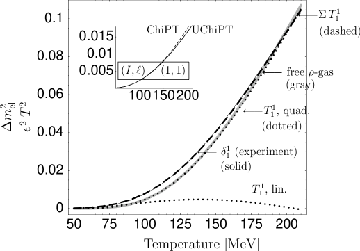
Figure 8: Main plot: Contribution to $m_{\rm el}^{2}$ in the $(I,\ell)=(1,1)$-channel of $\pi\pi$ scattering. Solid line: From experimental phase shift. Dotted lines: Terms linear and quadratic in $T$ from Eq. (LABEL:mel_rhoex) with $T$ from a unitary $\rho$ exchange model. Dashed line: Sum of linear and quadratic term. Gray line: free $\rho$-gas (Boltzmann).
Insert: With $T$ from the LO chiral Lagrangian. Dashed line: Tree level. Solid line: Unitarization with $K$-matrix.

Obviously the contribution from the quadratic term (“$T_{1}^{1}$, quad.”) is dominant, and adding the linear (“$T_{1}^{1}$, lin.”) and quadratic terms we obtain good agreement with the result from the $\delta_{1}^{1}$ experimental phase shift. This is to be expected as $T_{1}^{1}$ fits vacuum data well. Note that the linear term alone vastly underpredicts the electric mass. Thus the imaginary part of the amplitude is essential for the proper description of the fluctuations.

Furthermore, the electric mass from the free $\rho$-gas (Boltzmann statistics) (gray line, Fig. 8) agrees well with the results from the experimental phase shift and unitary $\rho$-model. Indeed, it can be shown that the $\pi\pi$-interaction via unitary $s$-channel $\rho$-exchange in the limit of vanishing width leads to a contribution to $\log Z$ equal to that of a free $\rho$-gas Welke:1990za ; Dashen:1974jw . In this limit $\delta_{1}^{1}(E)=\pi\,\Theta(E-m_{\rho})$ allowing for an explicit evaluation of Eq. (35) in the Boltzmann approximation. For Bose-Einstein statistics the situation is more complicated. In Ref. Dashen:1974jw it has been shown for meson-baryon interaction that also in this case the interaction of two particles via a narrow resonance $N^{*}$ leads to the same grand canonical potential as from a free $N^{*}$-gas with the corresponding Fermi-statistics for $N^{*}$; however, the proof requires a self-consistent medium modification of the $N^{*}$ width and a consideration of larger classes of diagrams.

While in our toy model we could simply restore unitarity by introducing a $\rho$ width, in a more complete calculation this is considerably more difficult. For example, using a $\rho$-propagator with a width in the diagrams of Figs. 3 and 4 leads to additional photon couplings to the intermediate pion loops, which generate the $\rho$-width. This is simply a consequence of gauge invariance (see Appendix C.4). Therefore, introducing unitary amplitudes while maintaining gauge invariance is a non-trivial task.

An alternative approach to assess the role of unitarity is to unitarize a given amplitude using the $K$-matrix approach (see, e.g. Weise ). This approach does not add any additional dynamics, and therefore provides a good estimator on the importance of unitarity alone. Using the $K$-matrix approach we can in principle take any of the interactions discussed in this paper. Here we choose the interaction in the $(1,1)$-channel from the LO chiral Lagrangian given in Eq. (6). Details of the calculation can be found in Appendix B.2. Maintaining gauge invariance in a $K$-matrix unitarization scheme requires special care and is beyond the scope of this paper. Ignoring this issue, we can compare the electric mass from the unitarized version using Eqs. (56,35,37) with the tree level amplitude using $T_{1}^{1}$ from Eq. (55) and then Eqs. (39,35,37). The results are plotted in the insert of Fig. 8 and show only a small correction due to unitarization.

Consequently, unitarity by itself is not as crucial as the dynamics which generates the resonance. In other words as long as the phase shift is slowly varying with energy unitarity corrections are small. A resonant amplitude on the other hand corresponds to a very rapidly varying phase-shift. Since it is the derivative of the phase-shift which enters the density expansion, resonant amplitudes are expected to dominate. Consequently, a resonance gas should provide a good leading order description of the thermodynamics of a strongly interacting system.

Note that the unitarized amplitude $T_{(u),1}^{1}$ from Eq. (55) corresponds to a unitarization via the Bethe-Salpeter equation in the limit where the real parts of the intermediate $\pi\pi$-loops are neglected; the freedom in the choice of the real part (loop regularization) can be used to fit to experimental phase shifts, which in turn introduces the missing dynamics (see, e.g., Refs. Oller:2000ma ; Doring:2004kt ) This should lead to more reliable predictions in_preparation .

To conclude this analysis of the density expansion, it appears that the low density expansion of Eq. (35), using experimental phase shifts, will give the most reliable results, while a simple hadron gas calculation should provide a reasonable first estimate for the fluctuations of a system. Finally, there are certain features of the $\rho$ model from Sec. V which can not be taken into account in the low density expansion: The $\rho\rho\pi\pi$ and $(\gamma)\gamma\rho\rho$ interactions discussed in Sec. V (Fig. 4) are a consequence of the $\rho$ being treated as a heavy gauge particle; these features will be missed in the low density or virial expansion in which the $\rho$ is not more than a resonant structure in the $\pi\pi$ amplitude. These considerations will be taken into account in the final numerical result from Sec. VIII.

VI.2 Numerical results for the interacting pion gas

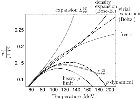
Figure 9: CF or electric mass for the interacting $\pi\pi$ system. The ${\cal L}_{\pi\pi}^{(2)}$, ${\cal L}_{\pi\pi}^{(4)}$ calculations are from Ref. Eletsky:1993hv and the conventional virial expansion (Boltzmann statistics) reproduces results from Ref. Eletsky:1993hv .

In Fig. 9 the results so far obtained are compared to Ref. Eletsky:1993hv (gray dashed lines). The electric mass for pions interacting in the heavy $\rho$ limit from Sec. IV.2 is indicated with the dotted line. Taking into account that the interaction from Eq. (16) is around 3/2 times stronger than the one from the LO chiral Lagrangian, the calculation is consistent with the ${\cal L}_{\pi\pi}^{(2)}$ calculation from Ref. Eletsky:1993hv which we have also checked analytically. The result for dynamical $\rho$ exchange (black dashed line) contains the contributions from free pion and $\rho$ gas and the diagrams from Fig. 5 (b), (c), and (d). The difference to the heavy $\rho$ limit shows the importance of the $\rho$ as an explicit degree of freedom in the heatbath.

Up to $T\sim 130$ MeV the dynamical $\rho$ exchange contributes with the same sign as the virial expansion from Ref. Eletsky:1993hv although they differ largely in size due to the lack of imaginary part in the loop calculation, especially in the $(I,\ell)=(1,1)$-channel as discussed above. Also the $\rho$-model does not describe the $(I,\ell)=(2,0)$ amplitude very well.

For the low density expansion from Eq. (35) and the virial expansion from Eq. (34) we use the phase shifts from Ref. Welke:1990za . Note that there is a partial cancellation from the $\delta_{1}^{1}$ and $\delta_{0}^{2}$ partial waves Eletsky:1993hv .

The ${\cal L}_{\pi\pi}^{(4)}$ calculation from Ref. Eletsky:1993hv , which of course contains also the ${\cal L}_{\pi\pi}^{(2)}$ contribution, shows a very distinct result. The reason is twofold: on one hand, unitarity is not preserved (see discussion in Sec. VI.1). On the other hand, the thermal loops in the ${\cal L}_{\pi\pi}^{(4)}$ calculation pick up high c.m. momenta where the theory is no longer valid and the dependence of the NLO interaction on high powers of momenta introduces artifacts. Note that the size of the correction from ${\cal L}_{\pi\pi}^{(4)}$ alone is larger than the one from ${\cal L}_{\pi\pi}^{(2)}$ for $T>80$ Mev.

The results for the observable $D_{S}$ from Eq. (4) are displayed in Fig. 10. Corrections to the entropy are included: from Eq. (29) for the heavy $\rho$ limit, from Eq. (58) for the case with dynamical $\rho$ and from Eq. (37) for the low density expansions.

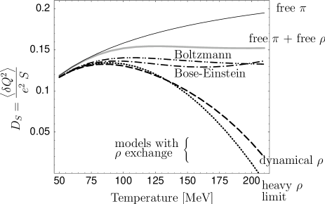
Figure 10: $D_{S}$ from Eq. (4) for the interacting $\pi\pi$ system. The heavy $\rho$ limit from Eqs. (28,29) includes the contribution from the free $\pi$ gas. The contributions from free $\pi$ and free $\rho$ gases are included for the result from Eqs. (65,67,68), the latter indicated as ”dynamical $\rho$”. The virial and density expansions are indicated according to their underlying particle statistics with ”Boltzmann” and ”Bose-Einstein”, respectively.

For the thermal loops, indicated by ”models with $\rho$ exchange”, $D_{S}$ is suppressed. This is due to the large negative correction to $\left\langle\delta Q^{2}\right\rangle$ as has been seen in Fig. 9. The virial expansion and the density expansion coincide better with each other than in Fig. 9 and can be roughly approximated by a gas of noninteracting pions and rhos.

Having contrasted virial expansions and dynamic $\rho$ model in Sec. VI.1, the most realistic results for CF and $D_{S}$ for the interacting $\pi\pi$ system are given by the Bose-Einstein density expansion from Eq. (35). While this result is somewhat below the estimate of a gas of free pions and $\rho$-meson, it is nowhere near the value of $D_{S}^{QGP}\simeq 0.034$ for the quark gluon plasma.

VII Higher order corrections

Both the density expansions and $\rho$ models from the last sections are quadratic in density, i.e., the statistical factor $n$. However, at the temperatures of the hadronic phase higher effects in density play an important role. Virial expansions become complicated beyond the second virial coefficient and no experimental information exists on three body correlations. Performing resummations is, therefore, of interest. This will include the density and strong coupling $g$ to all orders. Of course, this can not be done in a systematic way; resummations only contain certain classes of diagrams at a given order in perturbation theory. In all resummations, $\log Z$ is calculated at finite $\mu$ and then Eq. (22) is applied in order to obtain the electric mass. We have convinced ourselves in Sec. V that this is a charge conserving procedure.

We start with two natural extensions of the basic interaction diagram (a) in Fig. 5, displayed in Fig. 11 (n) and (r) using for both of them the effective interaction of the heavy $\rho$ limit from Eq. (16). Alternatively, one can use the LO chiral Lagrangian from Eq. (6). As found in Sec. III, results for the dominant part of this interaction are obtained by simply multiplying $g$ in the following by a factor of $2/3$. However, one should keep in mind the unitarity problems of these simplified point-like interactions which have been addressed in Sec. VI.1.

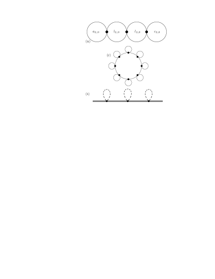
Figure 11: Resummation schemes: necklace (n) and ring (r). Below, the tadpole medium correction of the $\rho$ propagator is displayed (t).

For the calculation of diagram (n) we utilize an equation of the Faddeev type. The Faddeev equations, usually used in three-body scattering processes as in Ref. Doring:2004kt in a different context, are an easy way to sum processes whose elementary building blocks are of different types, as in this case loops of neutral pions with chemical potential $\mu=0$ and charged loops:

$$\log Z_{({\rm n})}(\mu) = \frac{1}{2}\;\beta V\left(\frac{1}{2}\;a_{0}\;b_{\pm}+a_{\pm}\left(b_{\pm}+b_{0}\right)\right)$$

$$b_{\pm} = g^{\prime}c_{\pm}+g^{\prime}l_{\pm}\left(b_{\pm}+b_{0}\right)$$

$$b_{0} = \frac{1}{2}\;g^{\prime}c_{0}+\frac{1}{2}\;g^{\prime}l_{0}\;b_{\pm}$$ (41)

with $g^{\prime}=-g^{2}/m_{\rho}^{2}$. The first loop in the chain is labeled $a$, the last one $c$, and $l$ means an intermediate loop. The indices ”$\pm$” and ”$0$” label charged and uncharged loops, respectively. It is instructive to expand Eq. (41) loop by loop which shows that the structure indeed reproduces all sequences of charged and uncharged loops, of all lengths. There is a symmetry factor of $1/2$ for every loop of neutral pions and a global factor of $1/2$ for every pion chain. The solution of Eq. (41) is found in Appendix E. The result of resummation (n) is plotted in Fig. 12 together with its expansion up to $g^{2}/m_{\rho}^{2}$ (dashed line) and up to $g^{4}/m_{\rho}^{4}$ (dotted line).

Figure 12: Left panel, main plot: Resummations (n) and (r) from Fig. 11 and their expansions up to $g^{2}/m_{\rho}^{2}$ (dashed line) and up to $g^{4}/m_{\rho}^{4}$ (dotted line) which are the same for (n) and (r). Insert: resummation (t), for order $g^{4}/m_{\rho}^{4}$ and higher. Right panel: CF over entropy, $D_{S}$. Result for heavy $\rho$ limit and dynamical $\rho$ as in Fig. 10. The result including the resummations (see text) is shown as the dashed dotted line ($\Sigma^{\prime}$).

The summation (r) of Fig. 11 with the interaction from Eq. (16) exhibits a symmetry factor of $1/N$ for a ring with $N$ ”small” loops (see Fig. 11) which after summing over $N$ leads to the occurrence of a logarithmic cut in the zero-component $p^{0}$ of the momentum of the ”big” loop. Due to this obstacle for the contour integration method Ka1989 , usually only the static mode $p^{0}=0$ is calculated, although new studies overcome this problem Liao:2002kp . In the present approach, we can calculate the ring with $N$ ”small” loops explicitly before summing over $N$. This avoids, thus, the problem of the logarithm at the cost of having to cut the series at some $N_{{\rm max}}$. On the positive side, all modes are included, and not only the $p^{0}=0$ static contribution. The result up to eight ”small” loops has already converged up to $T\sim 200$ MeV and is displayed in Fig. 12 as (r). The explicit solution can be found in Appendix E.

Note that in the resummation schemes we do not consider the vacuum parts of the loops, i.e. we do not renormalize the vacuum amplitude. This excludes potential double counting issues in the final numerical results in Sec. VIII where resummations and density expansion are added: Renormalizations of the vacuum amplitude are supposed to be be included in the phase shifts that are used in the density expansion.

There is an additional resummation scheme that sums up the $\rho\rho\pi\pi$ interaction required by the gauge invariance of the $\rho$ (see Eq. (13)): One can consider diagram (b) and (c) of Fig. 5, dress the $\rho$ propagator as indicated in (t) of Fig. 11, and finally take the heavy $\rho$ limit as in Sec. III. This leads to the same result as a renormalization of the static $\rho$ propagator $-1/m_{\rho}^{2}$ of diagram (a) in Fig. 5 for the $\pi\pi$ interaction in the heavy $\rho$ limit: The resummed pion tadpoles can be incorporated by a mass shift,

$$m_{\rho^{\pm}}^{2}\to m_{\rho}^{2}+\frac{g^{2}}{4}(U_{+}+U_{-}+2D),\quad m_{\rho^{0}}^{2}\to m_{\rho}^{2}+\frac{g^{2}}{2}(U_{+}+U_{-})$$ (42)

for charged and neutral $\rho$. The contribution to $m_{\rm el}$ from this modification is shown in the insert of Fig. 12 as (t). The thermal $\rho_{0}$ mass from Eq. (42) at $\mu=0$ is $m_{\rho_{0}}=824$ MeV at $T=170$ MeV which is slightly more than in other studies Sarkar:1997aa . This is certainly due to the omission of the $\rho\to\pi\pi\to\rho$ selfenergy which also contributes and is required by the gauge invariance of the $\rho$-meson. In the counting of the present study, the $\rho\to\pi\pi\to\rho$ selfenergy is statically included in the resummation (n) of Fig. 11.

To the right in Fig. 12 the normalized CF over entropy, $D_{S}$ from Eq. (4), are plotted. For comparison, the result at $g^{2}$ from the dynamical $\rho$-exchange (see Fig. 10) is shown with the dashed line. We include now the resummation (n) but only with three or more loops, or in other words, at $g^{4}$ and higher in the interaction in order to avoid double counting with the $g^{2}$ contribution. We have already seen in Fig. 12, left panel, that both resummations (n) and (r) contain the same diagram at order $g^{4}$ (linear chain of three loops). Thus, again in order to avoid double counting, we include the resummation (r) requiring at least three of the ”small” loops, see Fig. 11; this means that only contributions of order $g^{6}$ and higher are included. Finally, we add the resummation (t) including the orders $g^{4}$ and higher, which again avoids double counting of the $g^{2}$-contribution. Summing in this way the resummations to the $g^{2}$-result (dashed line) for both $\left\langle\delta Q^{2}\right\rangle$ and $S$, the resulting $D_{S}=\left\langle\delta Q^{2}\right\rangle/S$ is indicated as $\Sigma^{\prime}$ with the dashed-dotted line in Fig. 12.

The resummations have a large effect on $\left\langle\delta Q^{2}\right\rangle$ (see Fig. 12, left) whereas their effect on the entropy is much smaller; the entropy is efficiently suppressed for higher orders in the coupling. This explains, why the result $\Sigma^{\prime}$ shows such a large difference compared to the results at order $g^{2}$ (dashed line).

For the resummations (n) and (r), we have ensured that we recover the results from Eqs. (28) and (30) at the same order of the interaction. We have also verified that the results from Ref. Gale:1990pn at external momentum $p$ of the $\rho$ being zero $(p^{0}=0,{\bf p}\to 0)$ match the $\rho$ self energies at $\mu=0$ that are implicitly or explicitly contained in the resummations (n) and (t).

A possible extension of the diagrams discussed here is given by resummations of super-daisy type: the pion propagator is dressed by a series of pion tadpoles; the propagator of the tadpole loop itself is again dressed which constitutes a self consistency condition. E.g., this leads to a thermal mass of the pion $m_{\pi}\sim 170$ MeV at $T\sim 170$ Mev. However, one should realize that the lower orders in the coupling $g$ of a super-daisy expansion are already covered by the resummations considered before: it is easy to see that the super-daisy resummation introduces additional diagrams only at order $g^{8}$ and higher ($g^{6}$ and higher for resummation (t)) and, thus, can be neglected.

VII.1 Extension to $\bm{SU(3)}$

In order to obtain a more realistic model for the grand canonical partition function, the leading contributions from the interaction of the full $SU(3)$ meson and vector meson octets is considered. Obviously, the leading contribution to the CF from strange degrees of freedom is simply the free kaon gas. Here we want to discuss corrections due to interactions of kaons with pions. The most important of those is the resonant $p$-wave interaction involving an intermediate $K^{*}(892)$ meson. This is quite analogous to the $\rho$ meson in the $\pi\pi$ case, discussed previously. The $\Phi$ meson, on the other hand, only enters if interactions between kaons are considered. These are sub-leading as pions are more abundant and thus $\pi K$ interactions are more important.

As in the previous sections we describe the meson-meson interaction by dynamical vector meson exchange, second, by an effective interaction, and, third, by realistic phase shifts via a relativistic Bose-Einstein density expansion. For processes which contain at least one pion, the dynamical vector meson exchange is mediated by the $K^{*}(892)$. The effective contact interaction is taken from the LO chiral meson-meson Lagrangian in its $SU(3)$ version, ${\cal L}_{\pi K}^{(2)}$ for the $\pi K$-interaction. The density expansion of $\pi K$ scattering is obtained following the same steps as in Sec. VI. Details of the calculations are summarized in Appendix F.

Figure 13: Corrections to the electric mass or CF, $\left\langle\delta Q^{2}\right\rangle/(e^{2}VT^{3})$ for $\pi K$ interaction. The density and virial expansions are from Eqs. (100) and (102), respectively. The loop expansions ”$\pi K$ dynamical” and ”$\pi K$ contact” are from Eqs. (97,98) and (99), respectively. The solid line shows the electric mass of a gas of free $\kappa(800)$, $K^{*}(892)$, $K_{0}^{*}(1430)$, and $K_{2}^{*}(1430)$ mesons.

In Fig. 13 the CF from the different models are shown. For the virial and density expansion the phase shifts have been taken from the parametrization of Ref. Aston:1987ir for the attractive channels $\delta_{0}^{1/2},\delta_{1}^{1/2},\delta_{2}^{1/2}$, corrected for the parameters of the $K_{0}^{*}(1350)$ resonance (nowadays, $K_{0}^{*}(1430)$ in the PDG Eidelman:2004wy ) as reported in Ref. Venugopalan:1992hy . The repulsive $\delta_{0}^{3/2}$ phase shift is from Ref. Estabrooks:1977xe . The phase shifts plotted in Fig. 4 of Venugopalan:1992hy up to $s^{1/2}=1$ GeV have been reproduced.

The situation resembles the case of $\pi\pi$ scattering from Fig. 9: Thermal loops with dynamical vector exchange or with effective interaction via ${\cal L}_{\pi K}^{(2)}$ show large discrepancies to the virial and density expansions, this time even more than in the $\pi\pi$ case. The reasons are similar as those found in Sec. VI.1: The repulsive $(I,\ell)=(3/2,0)$ partial wave is not well described by $\pi K$ scattering via $K^{*}(892)$ and unitarity problems of the thermal loops show up. The contributions from both the virial expansion and the low density expansion are large compared to the virial corrections in the $\pi\pi$ sector (see Fig. 9). This seems surprising as in the $\pi K$ system the kaon has a large mass which should suppress contributions kinematically. However, in the considered channels of $\pi K$ scattering, four resonances are present, $\kappa(800)$, $K^{*}(892)$, $K_{0}^{*}(1430)$, and $K_{2}^{*}(1430)$ and we know from Sec. VI.1 that resonances give a large positive contribution to $m_{\rm el}$. The electric masses from these resonances, treated as free gases (Boltzmann), is plotted in Fig. 13 with the solid line. We find the same pattern as in the discussion of Fig. 8 for the free $\rho$: the virial corrections from resonant phase shifts are well described by a free gas of the same resonances. Furthermore, the repulsive $\delta_{0}^{3/2}$ phase shift is very small.

As the outcome for the density expansion in Fig. 13 shows, the inclusion of Bose-Einstein statistics is important (compare to the virial expansion which uses Boltzmann statistics). We consider the density expansion to provide the most reliable prediction.

VIII Numerical results

In the discussions in Secs. VI.1 and VII.1 good reasons have been found that at quadratic order in density $n$ the Bose-Einstein density expansion gives the most realistic results. For the final numerical results we include therefore the $\pi\pi$ and the $\pi K$ density expansion from Eqs. (35) and (100).

Figure 14: Final results for charge fluctuations (electric mass) and $D_{S}$. Results of the Bose-Einstein density expansions with the dashed-dotted lines. Adding $\rho\rho\pi\pi$ and $K^{*}K^{*}\pi\pi$ contributions, the resummations, and free mesons up to 1.6 GeV, the results are indicated with the dashed lines. For comparison, $m_{\rm el}^{2}$ and $D_{S}$ from free mesons alone, without any interactions, are also plotted (dotted lines).

The dashed-dotted lines in Fig. 14 show electric mass and normalized charge fluctuations $D_{S}$ from Eq. (4) for the sum of the two density expansions. At order $n^{2}$, there are additional photon selfenergy diagrams with $(\gamma)\gamma\rho\rho$ and $\rho\rho\pi\pi$ vertices from Fig. 4. As discussed at the end of Sec. VI.1 these contributions are not included in the density expansion but a consequence of the $\rho$ being introduced as a heavy gauge field. The same applies to the $K^{*}K^{*}\pi\pi$ diagram (d) from Eq. (98). Thus, we include these additional contributions for $\left\langle\delta Q^{2}\right\rangle$ and $S$.

At higher orders in density one has to rely on resummation schemes. Including the resummations in the final results does not to lead to double counting: Resummations at order $g^{4}$ and upwards in the strong coupling correspond to diagrams with three and more loops and, thus, to contributions higher than quadratic in density. We include (with $g^{4}$ and higher) the summations (n), (r), and (t) from Sec. VII. Note that for $m_{\rm el}$ there is a partial cancellation of sizable contributions from the resummations and the $(\gamma)\gamma\rho\rho$, $\rho\rho\pi\pi$, $K^{*}K^{*}\pi\pi$ diagrams.

In order to obtain a more realistic picture, we also include as free gases all mesons from the PDG Eidelman:2004wy which have not been considered so far, up to a mass of 1.6 GeV. Note that we do not add free mesons that have the same quantum numbers as the density expansions namely $\sigma(600)$, $\rho(770)$, $\kappa(800)$, $K^{*}(892)$, $K_{0}^{*}(1430)$, and $K_{2}^{*}(1430)$. We have seen in Sec. VI.1 that their contribution via phase shifts in the density expansions is roughly of the size as if they had been included as free particles. Adding all contributions mentioned, the results are indicated with the dashed lines in Fig. 14.

Compared to the density expansions the final results do not change much. The influence of heavier mesons than those considered in this study is, thus, well controlled. Many of the heavier resonances that have been added here as free gases are axials which decay into three particles. To include them in a density expansion would require the consistent treatment of three body correlations.

Concluding, we can assign $D_{S}\simeq 0.09$ for temperatures $120<T<200$ MeV which coincides (incidentally) quite well with the result if one simply considers free, noninteracting, mesons up to masses of $1.6$ GeV. The latter case is indicated with the dotted lines in Fig. 14.

Theoretical uncertainties in the present study arise from the omission of diagrams such as the (small) eye shaped diagram mentioned in Ref. Eletsky:1993hv already at $g^{4}$. Furthermore, both resummations and density expansions are incomplete as they only partly include the in-medium renormalization of the resonances which drive the meson-meson scattering, such as the $\sigma(600)$, $f_{0}(980)$, or the $\rho(770)$ itself Dashen:1974jw ; Gale:1990pn . In this context one can think of a more complete microscopical model: We have found in Sec. V and VI.1 that unitarity and a good description of the vacuum data up to high energies and in all partial waves are important. Such models exist, e.g., the chiral unitary approach from Ref. Oller:2000ma . The medium implementation of such a model has been done in a different context, see Dobado:2002xf ; GomezNicola:2002an and references therein. A generalization of the virial expansion from Ref. Pelaez:2002xf to finite chemical potential and including Bose-Einstein statistics, as carried out here, would be feasible in principle. Such an ansatz in_preparation would allow to take simultaneously into account the medium renormalization of the (dynamically generated) resonances and the calculation of the grand canonical partition function at finite $\mu$ as needed for a calculation of $m_{\rm el}^{2}$.

IX Summary and Conclusions

For an estimate of charge fluctuations (CF) in the hadronic phase of heavy ion collisions, we have calculated the effect of particle interactions. For the perturbative expansion up to two thermal loops, the $\pi\pi$ interaction has been described by vector meson exchange. The correlations induced by a dynamical $\rho$ have been found significant by comparing to an effective theory where the $\rho$ is frozen out.

The photon self energies are charge conserving and shown to be equivalent to the loop expansion of the grand canonical partition function at finite chemical potential. We have pointed out that the inclusion of imaginary parts is essential for a proper description of the thermodynamics, especially if resonant amplitudes are involved. To second order in the density, it has been possible to include Bose-Einstein statistics in the conventional virial expansion. This ”density expansion” can change the conventional results significantly. Moreover, for real amplitudes, we could show the equivalence of the loop expansion and the density expansion at all temperatures. However, the inclusion of unitary (complex) amplitudes is more straightforward in the density (virial) expansion. To the extend that two-particle correlations are dominant, the density expansion with Bose-Einstein statistics is, thus, the method of choice as it provides the same statistics as the thermal loop expansion and unitarity is automatically implemented by the use of realistic phase shifts.

For an estimate of three- and higher particle correlations, a variety of summation schemes has been presented, all of which tend to soften the large first order correction of the thermal loop expansion. For the CF, higher order corrections have a large influence whereas higher orders for the entropy are small.

For the CF over entropy, $D_{S}$, it has been shown that the influence of heavy particles beyond the interactions considered are well under control; a final value of $D_{S}\simeq 0.09$ has been found for temperatures $120<T<200$ MeV. This result agrees quite well with the outcome from the free resonance gas, supporting the notion that resonant amplitudes dominate the thermodynamics. As lattice gauge calculations with realistic quark masses become available it would be interesting to see at which point these start to significantly deviate from a hadron gas.

Acknowledgments: This work was supported by the Director, Office of Science, Office of High Energy and Nuclear Physics, Division of Nuclear Physics, and by the Office of Basic Energy Sciences, Division of Nuclear Sciences, of the U.S. Department of Energy under Contract No. DE-AC03-76SF00098. It has also been supported by the Studienstiftung des Deutschen Volkes and the program Formación de Profesorado Universitario of the Spanish Government.

Appendix A From charge fluctuations to photon selfenergy in sQED

In this section, an outline for the proof of Eq. (3) for scalar QED is given. The argument follows Ref. Ka1989 where a similar connection is made for QED. If $\pi\pi$ contact interactions are included according to Eq. (18), the steps outlined below are similar, but lengthier, and Ward identities for four-point functions have to be determined.

CF are defined as $\left\langle\delta Q^{2}\right\rangle=\left\langle Q^{2}\right\rangle-\left\langle Q\right\rangle^{2}$, and the expectation values are calculated via the statistical operator of the grand canonical ensemble with the charge chemical potential $\mu\equiv\mu_{Q}$. One obtains immediately:

$$\langle\delta Q^{2}\rangle=e^{2}TV\;\frac{\partial}{\partial\mu}\langle\hat{{\mbox{\j}}}_{0}\rangle$$ (43)

with $\hat{{\mbox{\j}}}_{0}$ the zero-component of the conserved current, $\hat{Q}=\int\hat{{\mbox{\j}}}_{0}=V\hat{{\mbox{\j}}}_{0}$. The expectation value of $\hat{{\mbox{\j}}}_{0}=i(\phi^{\star}(\partial^{0}+ieA^{0})\phi-\phi(\partial^{0}-ieA^{0})\phi^{\star})$ can be expressed in terms of the propagator

$$\left(\frac{\partial\langle\hat{{\mbox{\j}}}_{0}\rangle}{\partial\mu}\right)_{T}=-\frac{\partial}{\partial\mu}T\sum_{\omega_{n}=-\infty}^{\infty}\int\frac{d^{3}{\bf p}}{(2\pi)^{3}}\;2(p^{0}-\mu)\;{\cal G}(p^{0},{\bf p})$$ (44)

where we have used $\mu=eA^{0}$ and the definition of the imaginary time propagator

$${\cal G}_{\alpha\beta}({\bf x}\tau;{\bf x}^{\prime}\tau^{\prime})=-{\rm Tr}[{{\hat{\rho}}_{G}\;{\rm T}_{\tau}[\phi_{K\alpha}({\bf x}\tau)\phi^{\dagger}_{K\beta}({\bf x}^{\prime}\tau^{\prime})]]}$$ (45)

where $T_{\tau}$ is the $\tau$-ordered product in the modified Heisenberg picture, see, e.g., Ref. FeWa , and the Fourier transform is at equal times $\tau$, $\tau^{+}$ and position ${\bf x=x^{\prime}}$. The $\mu$-dependence of the propagator is given by $p^{0}=i\,\omega_{n}-\mu$ where $\omega_{n}=2\pi i\,n\,T$. With this, the derivative can be rewritten as

$$\left(\frac{\partial\langle\hat{{\mbox{\j}}}_{0}\rangle}{\partial\mu}\right)_{T}=-\sum_{\omega_{n}=-\infty}^{\infty}T\int\frac{d^{3}{\bf p}}{(2\pi)^{3}}\left(-2{\cal G}(p^{0},{\bf p})-2p^{0}\;\frac{\partial}{\partial p_{0}}\;{\cal G}(p^{0},{\bf p})\right)$$ (46)

at zero chemical potential $\mu=0$. Using $\partial/\partial p^{0}{\cal G}=-{\cal G}(\partial/\partial p^{0}{\cal G}^{-1}){\cal G}$, the Ward identity in the differential form for scalar QED can be applied. The Ward identity connects the inverse propagator with the fully dressed vertex $\Gamma^{\mu}$ according to

$$e^{2}TV\left(\frac{\partial\langle\hat{{\mbox{\j}}}_{0}\rangle}{\partial\mu}\right)_{T} = T^{2}V\sum_{\omega_{n}=-\infty}^{\infty}\int\frac{d^{3}{\bf p}}{(2\pi)^{3}}\Big{[}2e^{2}{\cal G}(p^{0},{\bf p})-e(2p^{0}){\cal G}(p^{0},{\bf p})\Gamma^{0}({\bf p},\omega_{n}){\cal G}(p^{0},{\bf p})\Big{]}$$ (47)

$$= TV\big{(}\underbrace{\Pi^{00}_{D\;{\rm mat}}(k_{0}=0,{\bf k}\to{\bf 0})}_{\begin{picture}(10.0,40.0)\put(-40.0,0.0){ \includegraphics[width=85.35826pt]{eq_a5_1.eps}} \end{picture}}+\underbrace{\Pi^{00}_{C\;{\rm mat}}(k_{0}=0,{\bf k}\to{\bf 0})}_{\begin{picture}(10.0,40.0)\put(-40.0,0.0){ \includegraphics[width=85.35826pt]{eq_a5_2.eps}} \end{picture}}\big{)}.$$

Factors of $e$ and $p^{0}$ have been identified here with the bare $\gamma\gamma\pi\pi$ and $\gamma\pi\pi$ vertices. In the step from Eq. (46) to Eq. (47) we have generated three propagators from one, and it should be noted that this takes place inside the momentum integral and summation. Therefore, the limit in Eq. (3) has to be taken before summation and integration.

Appendix B Pion-pion interaction

B.1 Chiral $\bm{\pi\pi}$ interaction and vector exchange

In this section the effective pion-pion contact interaction from Sec. III and its connection to the chiral Lagrangian is discussed in more detail. For four pion fields the kinetic term of ${\cal L}_{\pi\pi}^{(2)}$ in Eq. (6) and the effective interaction in Eq. (16) have identical isospin and momentum structure. Comparing the overall coefficients leads to the result in Eq. (17) which differs from the KSFR relation by a factor of $3/2$. Studying the low energy behavior of both theories helps solve this puzzle of the obvious violation of the phenomenologically well-fulfilled KSFR relation. The $\pi\pi$ amplitude at threshold from the LO chiral Lagrangian Eq. (6) and the effective interaction Eq. (16) is given by

$$T_{\pi\pi}^{(2)}=-\;\frac{2m_{\pi}^{2}}{f_{\pi}^{2}},\quad T_{{\rm eff}}=-\;\frac{4g^{2}m_{\pi}^{2}}{m_{\rho}^{2}},$$ (48)

respectively which leads to the correct KSFR relation

$$2f_{\pi}^{2}g^{2}=m_{\rho}^{2}.$$ (49)

This is due to the mass correction term proportional to ${\cal M}$ in Eq. (6). This term, however, does not have any momentum structure and immediately becomes small at finite pion momenta compared to the kinetic term. It has no influence in the results of this study.

For finite pion momenta, higher order partial waves have to be included. We concentrate on the quantum numbers of the $\rho$-meson and obtain for $\pi\pi$ scattering via the LO chiral interaction in isospin $I=1$:

$$T^{1}_{\pi\pi}=\frac{-1}{f_{\pi}^{2}}\;(t-u)$$ (50)

which should be compared to the result from $\rho$-exchange from Eq. (12):

$$T^{1}({\rm dyn.}\;\rho) = g^{2}\left(\frac{s-u}{t-m_{\rho}^{2}}+2\;\frac{t-u}{s-m_{\rho}^{2}+im_{\rho}\Gamma(s)}+\frac{t-s}{u-m_{\rho}^{2}}\right),$$

$$T^{2}({\rm dyn.}\;\rho) = g^{2}\left(\frac{u-s}{t-m_{\rho}^{2}}+\frac{t-s}{u-m_{\rho}^{2}}\right)$$ (51)

where we have also given the result for $T^{2}$ for completeness, and $T^{0}$ is immediately obtained by crossing symmetry, $T^{0}=-2T^{2}$. Projecting out the $p$-wave in both results (50) and (51) by using

$$T^{I}_{\ell}(s)=\frac{1}{64\pi}\int_{-1}^{1}d(\cos\theta)\;P_{\ell}(\cos\theta)\;T^{I}(s,t,u)$$ (52)

for $(I,\ell)=(1,1)$, making an expansion in ${\bf p}_{\rm cm}^{2}$, and comparing the coefficients, leads to the relation $m_{\rho}^{2}-4m_{\pi}^{2}=3f_{\pi}^{2}g^{2}$ which shows again the deviation of 3/2 from the KSFR relation up to a correction from the pion mass. However, taking only the $s$-channel vector exchange, which is given by the second term of $T^{1}$ Eq. (51), we obtain after projection to the $p$-wave:

$$m_{\rho}^{2}-4m_{\pi}^{2}=2f_{\pi}^{2}g^{2}.$$ (53)

This is indeed the KSFR relation in Eq. (49) with some small correction which vanishes when $s$ is neglected against $m_{\rho}^{2}$ in the denominator of Eq. (51). Concluding, the restriction to $s$-channel vector exchange in $\pi\pi$ scattering restores the KSFR relation in the $p$-wave expansion of the scattering amplitude. However, $t$- and $u$-channel vector exchange is also present, and this leads to the effective interaction in Eq. (16) which is 3/2 times stronger than the interaction from the LO chiral Lagrangian.

Fig. 15 illustrates the behavior of the different theories together with data from Ref. Froggatt:1977hu :

Figure 15: $p$-wave isovector $\pi\pi$ interaction. Dots: Partial wave analysis from Ref. Froggatt:1977hu . Dashed line: ${\cal L}_{\pi\pi}^{(2)}$ calculation. Dashed-dotted line: ${\cal L}_{\pi\pi}^{(4)}$ calculation from Ref. Donoghue:1992dd . Solid line: Effective interaction from Eq. (16). Thin solid lines: Explicit $\rho$ exchange from Eq. (12) with and without (momentum dependent) width for the $\rho$.

The LO chiral Lagrangian underpredicts the strength of the experimental $T_{1}^{1}$ amplitude. In contrast, the interaction up to ${\cal L}_{\pi\pi}^{(4)}$ and the effective interaction from Eq. (16) describe better the data at low energies. The explicit $\rho$ exchange with width (thin line) delivers a good data description even beyond the $\rho$-mass.

One more remark is appropriate in the framework of this section: In the treatment of the $\rho$-meson as a heavy gauge field, the covariant derivative introduces the $\pi\rho$ interaction as we have seen in Sec. III. Additionally, the original $\pi\pi$ interaction from Eq. (6) remains in this derivative. In the present model, we have omitted this term, as has been also done, e.g., in Ref. Klingl:1996by . This leads to better agreement with the data in the $T_{1}^{1}$-channel and ensures the KSFR relation. It is possible to keep the original chiral interaction, but then additional refinements have to be added added as, e.g., in Ref. Cabrera:2000dx .

B.2 Unitarization of the $\bm{\pi\pi}$-amplitude with the $\bm{K}$-matrix

The $K$-matrix is defined via the $S$-matrix as

$$S_{K}(E)=\frac{1+i\,Q\,K}{1-i\,Q\,K},\quad K=-\,\frac{T_{\rm tree}}{16\pi\,E}$$ (54)

with the tree level amplitude $T_{\rm tree}$ from Eq. (50) and the c.m. momentum $Q$ from Eq. (36). The unitarized amplitude $T_{(u),1}^{1}$ which is given by

$$T_{(u),1}^{1}=\frac{T_{1}^{1}}{1+2i\,Q\,T_{1}^{1}/E},\quad T_{1}^{1}=-\frac{E^{2}-4m_{\pi}^{2}}{96\pi\,f_{\pi}^{2}}$$ (55)

can be parametrized via phase shift as

$$\delta_{1}^{1}=\frac{1}{2}\arctan\;\frac{-{\rm Re}\,T_{(u),1}^{1}}{\frac{E}{4Q}+{\rm Im}\,T_{(u),1}^{1}}.$$ (56)

Appendix C The $\bm{\rho}$-meson in the heatbath

C.1 Analytic results

The analytical expressions and numerical contributions from the set of gauge invariant diagrams in Fig. 3 are given which are obtained from the interactions from Sec. III. With

$$L_{\pm}\left(a,b\right):=\log\left|\frac{\left[m_{\rho}^{2}+\left(p\pm q\right)^{2}-\left(b\;\omega-a\omega^{\prime}\right)^{2}\right]\left[m_{\rho}^{2}+\left(p-q\right)^{2}-\left(b\;\omega+a\omega^{\prime}\right)^{2}\right]}{\left[m_{\rho}^{2}+\left(p\mp q\right)^{2}-\left(b\;\omega-a\omega^{\prime}\right)^{2}\right]\left[m_{\rho}^{2}+\left(p+q\right)^{2}-\left(b\;\omega+a\omega^{\prime}\right)^{2}\right]}\right|,$$ (57)

where $\omega^{2}=q^{2}+m_{\pi}^{2}$ and $\omega^{\prime 2}=p^{2}+m_{\pi}^{2}$, we obtain for the real parts of the diagrams in Fig. 3, left column:

$$\Pi_{({\rm 1a1})}^{00}(k_{0}=0,{\bf k\to 0}) = \;\frac{-e^{2}g^{2}}{\left(2\pi\right)^{4}m_{\rho}^{2}}\;\frac{\partial}{\partial\alpha}\;\frac{\partial}{\partial\beta}|_{\alpha=\beta=1}\int\limits_{0}^{\infty}dp\int\limits_{0}^{\infty}dq\;\frac{pq}{\alpha\beta\omega\omega^{\prime 3}}\;n[\omega]\;n\left[\alpha/\beta\;\omega^{\prime}\right]$$

$$\times \left[-8m_{\rho}^{2}\;pq+\left[(2m_{\pi}m_{\rho})^{2}-\left(m_{\rho}^{2}-\left(\left(\alpha/\beta\right)^{2}-1\right)\omega^{\prime 2}\right)^{2}\right]L_{-}\left(\alpha/\beta,1\right))\right],$$

$$\Pi_{({\rm 1a2})}^{00}(k_{0}=0,{\bf k\to 0}) = \;\frac{-e^{2}g^{2}}{2\left(2\pi\right)^{4}}\;\;\frac{\partial}{\partial\alpha}\;\frac{\partial}{\partial\beta}|_{\alpha=\beta=1}\int\limits_{0}^{\infty}dp\int\limits_{0}^{\infty}dq\;\frac{pq}{\left(\omega\omega^{\prime}\right)^{2}}\;n[\beta\omega]\;n\left[\alpha\omega^{\prime}\right]$$

$$\times \left[4m_{\pi}^{2}-m_{\rho}^{2}+2\left((\beta^{2}-1)\omega^{2}+(\alpha^{2}-1)\omega^{\prime 2}\right)-\frac{1}{m_{\rho}^{2}}\left((\alpha^{2}-1)\omega^{\prime 2}-(\beta^{2}-1)\omega^{2}\right)^{2}\right]$$

$$\times L_{+}\left(\alpha,\beta\right),$$

$$\Pi_{({\rm 4a})}^{00}(k_{0}=0,{\bf k\to 0}) = \;\frac{-e^{2}g^{2}}{\left(2\pi\right)^{4}m_{\rho}^{2}}\;\frac{\partial}{\partial\alpha}|_{\alpha=1}\int\limits_{0}^{\infty}dp\int\limits_{0}^{\infty}dq\;\frac{pq}{\alpha\omega\omega^{\prime 3}}\;n[\omega]\;n[\alpha\omega^{\prime}]$$

$$\times \left[-8m_{\rho}^{2}\;pq+\left[(2m_{\pi}m_{\rho})^{2}-\left(m_{\rho}^{2}-(\alpha^{2}-1)\omega^{\prime 2}\right)^{2}\right]L_{-}(\alpha,1)\right],$$

$$\Pi_{({\rm 5a})}^{00}(k_{0}=0,{\bf k\to 0}) = \frac{6e^{2}g^{2}}{\left(2\pi\right)^{4}m_{\rho}^{2}}\;\frac{\partial}{\partial\alpha}|_{\alpha=1}\;\int\limits_{0}^{\infty}dp\int\limits_{0}^{\infty}dq\;\frac{pq}{\omega\omega^{\prime 2}}\;n[\omega]\;n\left[\alpha\omega^{\prime}\right]$$

$$\times \left[-\alpha\omega^{\prime}\left(m_{\rho}^{2}+(1-\alpha^{2})\omega^{\prime 2}\right)L_{-}\left(\alpha,1\right)+\omega\left(m_{\rho}^{2}+(\alpha^{2}-1)\omega^{\prime 2}\right)L_{+}\left(\alpha,1\right)\right],$$

$$\Pi_{({\rm 6a})}^{00}(k_{0}=0,{\bf k\to 0}) = \;\frac{-3e^{2}g^{2}}{\left(2\pi\right)^{4}m_{\rho}^{2}}\;\int\limits_{0}^{\infty}dp\int\limits_{0}^{\infty}dq\;\frac{pq}{\omega\omega^{\prime}}\;n[\omega]\;n\left[\omega^{\prime}\right]$$

$$\times \left[-\left(m_{\rho}^{2}-\omega^{2}-\omega^{\prime 2}\right)L_{-}\left(1,1\right)+2\omega\omega^{\prime}L_{+}\left(1,1\right)\right],$$

$$\log Z_{{\rm(en1)}} = \frac{3g^{2}V}{4T\left(2\pi\right)^{4}}\;\int\limits_{0}^{\infty}dp\int\limits_{0}^{\infty}dq\;\frac{pq}{\omega\omega^{\prime}}\;n[\omega]\;n\left[\omega^{\prime}\right]\left[-8pq+\left(4m_{\pi}^{2}-m_{\rho}^{2}\right)L_{-}\left(1,1\right))\right].$$ (58)

In these expressions the poles from the $\rho$-propagator have been omitted as discussed in Appendix C.2. The use of derivatives in Eq. (58) cures infrared divergences which occur (see Appendix C.2). The logarithmic pole in the numerically relevant integration regions for $p$ and $q$ is in all cases is given by

$$m_{\rho}^{2}+(p-q)^{2}-\left(b\;\omega+a\;\omega^{\prime}\right)^{2}=0$$ (59)

where $a,b$ take values according to the arguments of $L_{\pm}(a,b)$ of Eqs. (57,58). The singularity leads to an imaginary part which we neglect. The issue of imaginary parts is discussed in Sec. VI.1. The diagrams from the second column of Fig. 3 are calculated straightforward with the results

$$\Pi^{00}_{(1c1)}=-\frac{e^{2}g^{2}}{m_{\rho}^{2}}\;C^{2},\quad\Pi^{00}_{(5c1)}=-\frac{2e^{2}g^{2}}{m_{\rho}^{2}}\;CD,\quad\Pi^{00}_{(6c)}=-\frac{e^{2}g^{2}}{m_{\rho}^{2}}\;D^{2}$$ (60)

in the static limit ($k_{0}=0,{\bf k\to 0}$).

Fig. 16 shows the numerical results.

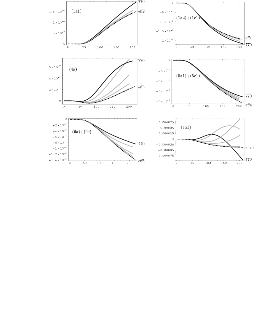
Figure 16: Numerical results for the diagrams from Fig. 3, Eq. (58) as a function of $T$ [MeV]. Selfenergy $\Pi/(e^{2}T^{4})$ in [MeV^-2] for all plots, except the correction to $Z$: $\log Z_{{\rm(en1)}}/(VT^{4})$ in [MeV]^-1. Results for different $m_{\rho}$ with solid lines. Dashed lines: Corresponding diagrams from the heavy $\rho$ limit, see Tab. 1 and Eq. (29).

For every diagram, the contribution of the dynamical $\rho$-meson at its physical mass of $m_{\rho}=770$ MeV (indicated with ”770”) is displayed. Additionally, the amplitudes for $\rho$-masses of $m_{\rho}^{i}=1070,1770,2770,10000$ MeV are evaluated, multiplying the result with $(m_{\rho}^{i}/m_{\rho})^{2}$ (gray lines). This would correspond to a $\rho$-meson with mass $m_{\rho}^{i}$ whose strong coupling $g$ is increased by $(m_{\rho}^{i}/m_{\rho})$. This is indeed equivalent to the heavy $\rho$ limit from Sec. III and convergence of the results from Eq. (58) towards the heavy $\rho$ limit of Sec. IV.2 (dashed lines) is observed. This convergence is, on the other hand, a useful tool to check the results from Eq. (58).

The large difference of both models at $m_{\rho}=770$ MeV in case of the diagrams (4a) and (eff3) is due to terms that partially cancel: diagram (eff3) $\sim D(2D-C)$. For the calculation of the entropy in Eq. (4), the correction to $\log Z$ is needed which is very different for diagram (eneff) and diagram (en1) as Fig. 16 shows. The discrepancy can be traced back to the different high energy behavior of the amplitudes. In any case, the total size of the entropy correction, compared to the result of the free pion gas, Eq. (24), is small and of no relevance for the final results.

C.2 Calculation of diagram (1a2)

The calculation of one of the diagrams from Fig. 3 is outlined in more detail. The evaluation of the other diagrams is carried out in an analog way, with the results given in Eqs. (58,60). For diagram (1a2) it is most convenient to treat the vertex correction first, that is given by the left side of the diagram. The external photon momentum has to be set to zero from the beginning of the calculation as has been shown in Appendix A; the matter part of the vertex correction reads for an external $\pi^{+}$:

$$\Gamma^{0}[k^{0}=0,{\bf k\to 0}] = \frac{2eg^{2}p^{0}}{\pi^{2}}\;\int\limits_{0}^{\infty}dq\;q^{2}\int\limits_{-1}^{1}dx\;\frac{1}{2\pi i}\int\limits_{-i\infty+\epsilon}^{i\infty+\epsilon}dq^{0}\;n[q^{0}]\;\frac{\left(q^{0}\right)^{2}}{\left((q^{0})^{2}-\omega^{2}\right)^{2}}$$ (61)

$$\times \frac{4m_{\pi}^{2}-m_{\rho}^{2}+2\left((p^{0})^{2}+(q^{0})^{2}-\omega^{2}-\omega^{\prime 2}\right)-\left(1/m_{\rho}^{2}\right)\left((p^{0})^{2}-(q^{0})^{2}+\omega^{2}-\omega^{\prime 2}\right)^{2}}{\left((p^{0}+q^{0})^{2}-\eta^{2}\right)\left((p^{0}-q^{0})^{2}-\eta^{2}\right)}$$

where the contour integration method of Ref. Ka1989 is used for the summation over Matsubara frequencies. In Eq. (61), $\omega^{2}=q^{2}+m_{\pi}^{2}$ and $\eta^{2}=p^{2}+q^{2}-2pqx+m_{\rho}^{2}$. A problem occurs when closing the integration contour in the right $q^{0}$ half plane: The residue at $\omega$ from the double pole of the two pion propagators at the same energy is given by

$${\rm Res}\;f(z)|_{z=\omega}=\lim_{z\to\omega}\frac{1}{(m-1)!}\frac{d^{m-1}}{dz^{m-1}}[f(z)(z-\omega)^{m}]$$ (62)

at $m=2$. The derivative also applies to the denominator in the second line of Eq. (61) from the $\rho$ propagator. The integrand exhibits then a divergence of the type

$$\Gamma[k^{0}=0,{\bf k\to 0}]\sim\int dq\;\frac{1}{a-q^{2}},\quad\mbox{at}\quad p^{0}=0.$$ (63)

The divergence affects only the zero-mode $p^{0}=0$, but when the pion lines are closed later on, in order to obtain diagram (1a2), the integrals in Eq. (61) are not defined any more, and one finds poles of the type $1/(a-{\bf q}^{2})$ in the three-momentum integration. This infrared divergence, for the external photon at $k=0$, occurs in diagrams that contain, besides two or more propagators at the same momentum, an additional propagator as in this case the one of the $\rho$-meson.

The complication can be most easily overcome with the introduction of additional parameters according to

$$\frac{1}{2\omega^{2}}\frac{\partial}{\partial\beta}|_{\beta=1}\;\frac{1}{(q^{0})^{2}-(\beta\omega)^{2}}=\frac{1}{\left((q^{0})^{2}-\omega^{2}\right)^{2}},$$ (64)

and performing the derivative numerically after the three-momentum integration. Still, singularities of the $1/q$ type remain, but they are well-defined by the $\epsilon$-prescription in the $q^{0}$-integral of Eq. (61). We can in this case, as well as in all other diagrams from Fig. 3, integrate the angle $x=\cos({\bf p,q})$ analytically, thus being left with logarithmic singularities, that are easily treated numerically with the help of Eq. (59).

It has been checked for all diagrams in Fig. 3 that the poles of the $\rho$-meson can be omitted: In Eq. (61) the denominator of the second line from the $\rho$-propagator produces two single poles in the right $q^{0}$ half plane. Taking these residues into account in the contour integration leads to deviations of less than 1 % of the result for the vertex correction, for all values of $(p^{0},{\bf p})$ and up to temperatures $T\sim 200$ MeV. Intuitively, this is clear since these poles produce a strong Bose-Einstein suppression $\sim n[m_{\rho}]$ and extra powers of $m_{\rho}$ in the denominator compared to the pion pole. This approximation is made for all results of Eq. (58). See also Sec. VI.1 where the approximation is again tested.

The rest of the evaluation of diagram (1a2) is straightforward up to the introduction of an additional derivative parameter in the same manner as above. As one can see in Fig. 3, a topologically different structure, diagram (1c1), is possible for the combination of two $\gamma\pi\pi$ and two $\rho\pi\pi$-vertices. This diagram is easily evaluated and has to be added.

C.3 The $\bm{\gamma\pi\rho}$ system at finite $\bm{\mu}$.

Explicit results for $\log Z$ from the diagrams (b), (c), and (d) from Fig. 5 are given from which the electric mass can be directly calculated using Eq. (22). As argued in the main text, the diagrams (b,c,d) from Fig. 5 lead to the same CF as all diagrams with dynamical $\rho$ from Figs. 3 and 4. For diagram (b), the result is

$$\log Z^{\pi\pi}_{{\rm(b)}}(\mu) = \frac{-g^{2}\beta V}{32}(U_{+}+U_{-})(U_{+}+U_{-}+4D)+\frac{g^{2}\beta V}{128\pi^{4}}\int\limits_{0}^{\infty}dp\int\limits_{0}^{\infty}dq\;\frac{pq\left(4m_{\pi}^{2}-m_{\rho}^{2}\right)}{\omega\omega^{\prime}}$$ (65)

$$\times \big{[}\left(n_{+}n[\omega^{\prime}-\mu]+n_{-}n[\omega^{\prime}+\mu]\right)\log_{1}+\left(n_{+}n[\omega^{\prime}+\mu]+n_{-}n[\omega^{\prime}-\mu]\right)\log_{2}\big{]}$$

with $U_{\pm}$ and $V_{\pm}$ from Eq. (31), $n_{\pm}=n[\omega\pm\mu]+2n[\omega]$, and

$$\log_{1}=\log\left[\frac{m_{\rho}^{2}+(p-q)^{2}-(\omega+\omega^{\prime})^{2}}{m_{\rho}^{2}+(p+q)^{2}-(\omega+\omega^{\prime})^{2}}\right],\;\log_{2}=\log\left[\frac{m_{\rho}^{2}+(p-q)^{2}-(\omega-\omega^{\prime})^{2}}{m_{\rho}^{2}+(p+q)^{2}-(\omega-\omega^{\prime})^{2}}\right],$$ (66)

with $\omega^{2}=q^{2}+m_{\pi}^{2}$, $\omega^{\prime 2}=p^{2}+m_{\pi}^{2}$, and $n$ the Bose-Einstein distribution. We have checked that $\log Z_{{\rm(b)}}(\mu=0)=\log Z_{{\rm(en1)}}$ from Eq. (58). The diagram (c) in Fig. 5 with

$$\log Z^{\pi\pi}_{{\rm(c)}}(\mu)=-\;\frac{g^{2}\beta V}{8m_{\rho}^{2}}\left(V_{+}-V_{-}\right)^{2}$$ (67)

is zero for $\mu=0$ and therefore $\log Z_{{\rm(c)}}$ does not contribute to the entropy but only to the CF.

The diagram (d) in Fig. 5 contains a $\rho\rho\pi\pi$ vertex that comes from Eq. (13). This interaction is required by the gauge invariance of the $\rho$ with the contribution to $m_{\rm el}$ given by

$$\log Z^{\pi\pi}_{{\rm(d)}}(\mu)=-\frac{3\beta Vg^{2}}{16}\left[(U_{+}^{\rho}+U_{-}^{\rho}+2D^{\rho})(U_{+}^{\pi}+U_{-}^{\pi}+2D^{\pi})-4D^{\rho}D^{\pi}\right].$$ (68)

The upper index for $U,D$ indicates which mass has to be used in the meson energy $\omega$ of Eqs. (21) and (31).

C.4 Charge conservation

In a calculation of CF the conservation of charge is essential and therefore gauge invariance of the diagrams must be ensured. The set of diagrams in Fig. 2 has been constructed using the Ward identity following the procedure outlined in Appendix A. They ought to be charge conserving by construction. Nevertheless, it is desirable to have an explicit proof. The diagrams from Fig. 2 represent the heavy $\rho$ limit of the ones with dynamical $\rho$-mesons in Fig. 3 as shown in Appendix C.1. Therefore, it is enough to show charge conservation for the latter.

From Ref. PeSc1995 we utilize the part of the proof that concerns closed loops. The main statement extracted from Ref. PeSc1995 is, adapted to the current situation: Define a diagram with one external photon at momentum $k$, not necessarily on-shell. By inserting another photon in all possible ways in the diagram, a set of new diagrams of photon selfenergy type emerges: For example, the four diagrams in Fig. 17

Figure 17: Elementary diagrams to be saturated with an additional photon in order to construct the selfenergy from Fig. 3.

lead to the photon self energies in the two left columns of Fig. 3 plus the (vanishing) diagrams (1c2), (4c), and (5c2) from Fig. 4, once saturated with an additional photon (we do not allow direct $\gamma\rho\rho$ and $\gamma\gamma\rho\rho$ vertices). The selfenergy diagrams $\Pi^{\mu\nu}_{i}$ constructed in this way are charge conserving, and $k_{\mu}\sum_{i}\Pi^{\mu\nu}_{i}=0$ for the sum over all diagrams.

For this statement, it has to be shown first that indeed the diagrams from Fig. 3, including all symmetry and isospin factors, turn out from the ones of Fig. 17. This short exercise reveals that there are two classes of selfenergy diagrams: one comes from inserting photons in diagrams (1) and (2) of Fig. 17 and the other one from inserting photons in (3) and (4). Thus, there are two separate gauge-invariant classes. In a second step, one has to show the statement from Ref. PeSc1995 for the current theory which is different from QED and richer in vertices of different type:

(I) The $\gamma\pi\pi$ couplings in Fig. 17 can be transformed into $\gamma\gamma\pi\pi$ couplings by inserting an additional photon. The $\rho\pi\pi$ vertex can be transformed into a $\gamma\rho\pi\pi$ vertex. These transformations which are a consequence of the momentum dependence of the vertices are essential for the proof.

(II) For this proof we do not allow direct $\gamma\rho\rho$ and $\gamma\gamma\rho\rho$ couplings. However, diagrams which include these couplings as in Fig. 4 form a disjoint gauge class anyway.

(III) The gauge invariance of the diagrams with dynamical $\rho$ in Fig. 3 survives in the heavy $\rho$ limit: According to Appendix C.1, the amplitudes at a $\rho$-mass of $m_{\rho}^{i}$ are multiplied by $(m_{\rho}^{i}/m_{\rho})^{2}$, with $m_{\rho}$ the physical mass. Then, the limit $m_{\rho}^{i}\to\infty$ is taken and the effective diagrams of Fig. 2 turn out. The gauge invariance of these diagrams follows.

This simple graphical proof demonstrates the charge conservation, and, turning the argument around, provides a useful tool to ensure that the amplitudes, including symmetry and isospin factors, have been correctly determined in Eqs. (58,60) and Tab. 1.

Appendix D Structure of the low density expansion

For a motivation of Eq. (35), we consider the general expression of Eq. (33) for the case of two interacting particles. This result is obtained in Dashen after carrying out the trace over particle states, i.e. two integrations over the momenta ${\bf p}_{1}$ and ${\bf p}_{2}$ of the interacting particles:

$$B_{2}(\mu=0) = -\;\frac{\beta}{2}\int\frac{d^{3}{\bf p}_{1}}{(2\pi)^{3}}\;\frac{1}{2\omega_{1}^{\prime}}\int\frac{d^{3}{\bf p}_{2}}{(2\pi)^{3}}\;\frac{1}{2\omega_{2}^{\prime}}\;e^{-\beta\omega_{1}^{\prime}}\;e^{-\beta\omega_{2}^{\prime}}\;T({\bf p}_{1},{\bf p}_{2})$$ (69)

where $\omega_{1,2}^{\prime}=\sqrt{{\bf p}_{1,2}^{2}+m_{\pi}^{2}}$. The momenta ${\bf p}_{1}$ and ${\bf p}_{2}$ are defined in the gas rest frame. For simplicity, we consider here only a real $T$-Matrix for the interaction and set $\mu=0$. The extension to finite $\mu$ and complex $T$ is straightforward. Note that in the current normalization, $T$ is connected to $T_{J}^{I}$ according to $T\to(32\pi)\;T_{J}^{I}$ (see Eq. (52)). The integrations in Eq. (69) can be rewritten in terms of the momentum of the 2-particle cluster, ${\bf k}={\bf p}_{1}+{\bf p}_{2}$, and the relative momentum in the two-particle c.m. frame, ${\bf Q}$, which implies a Lorentz boost along ${\bf k}$. Using the fact that

$$\int\frac{d^{3}{\bf p}_{1}}{2\omega_{1}^{\prime}}\;\int\frac{d^{3}{\bf p}_{2}}{2\omega_{2}^{\prime}}=\int\frac{d^{3}{\bf Q}\;d^{3}{\bf k}}{E\sqrt{E^{2}+{\bf k}^{2}}}\;,$$ (70)

where $E\equiv s^{1/2}$ is the total energy of the pions in the c.m. system, Eq. (69) can be rewritten with a result corresponding to Eq. (33). For the moment we ignore the symmetrization operator $A$ in Eq. (33) which will be taken care of below. The Lorentz boost of the statistical exponents in Eq. (69) is in this case easy to carry out and leads to the factor $e^{-\beta\sqrt{{\bf k}^{2}+E^{2}}}$ by noting that the invariant energy is given by $E^{2}=s=(\omega_{1}^{\prime}+\omega_{2}^{\prime})^{2}-{\bf k}^{2}$.

Obviously, no quantum statistical information has entered in Eq. (69). However, in Sec. VIIB of Ref. Dashen it is shown that the fermionic or bosonic nature of the particles can be (partly) included by summing over exchange diagrams, i.e., permutating the particles. The final result of this procedure is the replacement of the statistical factors $e^{-\beta\omega^{\prime}}$ in Eq. (69) by Bose-Einstein factors leading to

$$B_{2}(\mu=0) = -\;\frac{\beta}{2}\int\frac{d^{3}{\bf p}_{1}}{(2\pi)^{3}}\;\frac{1}{2\omega_{1}^{\prime}}\int\frac{d^{3}{\bf p}_{2}}{(2\pi)^{3}}\;\frac{1}{2\omega_{2}^{\prime}}\;\frac{1}{e^{\beta\omega_{1}^{\prime}}-1}\;\frac{1}{e^{\beta\omega_{2}^{\prime}}-1}\;T({\bf p}_{1},{\bf p}_{2}),$$ (71)

which formally have the appearance of Bose-Einstein factors as shown in Sec. VIIB of Dashen (see also the example in Sec. VIIC of Dashen ). As before in the evaluation of Eq. (69), we can use at this point Eq. (70). In order to obtain the final form of Eq. (35), finite charge chemical potential and complex $T$-matrix elements, projected over angular momentum, are straightforward introduced. Also, it is more convenient to express the pion scattering in terms of isospin amplitudes. The final result is shown in Eq. (35).

The Lorentz boost into the c.m. frame at velocity ${\bf v}={\bf k}/(E^{2}+{\bf k}^{2})$, implicitly contained in Eq. (70), has also to be carried out for the statistical factors in Eq. (71). Unlike in the simple case of Eq. (69), this leads to the slightly more complex expressions shown in Eq. (36). Note the boost is not essential but convenient as the scattering amplitude is easily obtained in the two-particle c.m. frame and some integrations can be carried out analytically.

Formally, exchange diagrams are included in Eq. (33) through the symmetrization operator $A$. Note, however, that in the standard form of the virial expansion, Eq. (34), effects from exchange diagrams are missing. This highlights again the difference between the virial expansion, Eq. (34), and the low density expansion in Eq. (35).

In fact, Eq. (71) is not an unfamiliar expression: Let us put $T=\lambda\equiv$const, i.e. using $\phi^{4}$ theory with ${\cal L}=-\lambda/4!\,\phi^{4}$, and calculate thermodynamic observables such as the pressure from $B_{2}$. Using the same interaction, we can compute the observables also from thermal loops in the imaginary time formalism (see e.g. Sec. V) at order $\lambda$. Results are identical. In Sec. VI.1 this agreement is reconfirmed for more complex interactions.

The observation of equivalence of the methods from Dashen and the thermal loop expansion is, to our best knowledge, novel; although in Eletsky:1993hv , using an effective range expansion for the amplitude, a similar equivalence has been found on the level of Eq. (34), i.e., without including Bose-Einstein statistics through exchange diagrams.

Appendix E Solutions for the resummations

An additional technical complication appears in the evaluation of Eq. (41) for the summation (n) when the structure of the vertices between $\pi^{\pm}\pi^{\pm}$-loops or $\pi^{0}\pi^{\pm}$-loops is inspected: The interaction of Eq. (16) leads to a Feynman rule of the form $\left(p^{2}+q^{2}+6pq\right)$ for the vertex between two charged pion loops of momenta $p$ and $q$, and of the form $\left(p^{2}+q^{2}\right)$ between a charged and a $\pi^{0}$-loop, always implying the corresponding shift $p^{0}\to p^{0}\pm\mu$ ($q^{0}\to q^{0}\pm\mu$) for the inclusion of finite chemical potential. Therefore, the loops can not be factorized easily in the way Eq. (41) suggests. In order to cast the resummations in a manageable from, we introduce for every term of the sum $\left(p^{2}+q^{2}+6pq\right)$ an entry in an additional index that runs from 1 to 3. The Eq. (41) is then to be read as a matrix equation in its variables. With the definitions

$$W_{\pm}=\frac{1}{\pi^{2}}\int\limits_{0}^{\infty}dq\;\omega\;n[\omega\pm\mu],\quad X_{\pm}=\frac{1}{\pi^{2}}\int\limits_{0}^{\infty}dq\;\omega^{2}n[\omega\pm\mu],$$ (72)

additional to the ones of Eq. (21) and (31), the entries of the Faddeev-like equations (41) can be cast in the form

$$a_{0} = \left(D,\;m_{\pi}^{2}D,\;0\right),$$

$$a_{\pm} = \frac{1}{4}\left(U_{+}+U_{-},m_{\pi}^{2}\left(U_{+}+U_{-}\right),\sqrt{6}\left(V_{-}-V_{+}\right)\right)$$

$$c_{0} = \left(\begin{array}[]{l}m_{\pi}^{2}D\\ D\\ 0\end{array}\right)$$ (76)

$$c_{\pm} = \frac{1}{4}\left(\begin{array}[]{l}m_{\pi}^{2}\left(U_{+}+U_{-}\right)\\ U_{+}+U_{-}\\ \sqrt{6}\left(V_{-}-V_{+}\right)\end{array}\right)$$ (80)

$$l_{0} = \left(\begin{array}[]{lll}C-3D&m_{\pi}^{2}(C-5D)&0\\ \frac{1}{m_{\pi}^{2}}\;(C-D)&C-3D&0\\ 0&0&0\end{array}\right)$$ (84)

$$l_{\pm} = \frac{1}{8}\left(\begin{array}[]{lll}W_{+}-3U_{+}+W_{-}-3U_{-}&m_{\pi}^{2}\left(W_{+}-5U_{+}+W_{-}-5U_{-}\right)&\sqrt{6}\left(3V_{+}-X_{+}-3V_{-}+X_{-}\right)\\ \frac{1}{m_{\pi}^{2}}\left(W_{+}-U_{+}+W_{-}-U_{-}\right)&W_{+}-3U_{+}+W_{-}-3U_{-}&\frac{\sqrt{6}}{m_{\pi}^{2}}\left(X_{-}-V_{-}-X_{+}+V_{+}\right)\\ \frac{\sqrt{6}}{m_{\pi}^{2}}\left(X_{-}-V_{-}-X_{+}+V_{+}\right)&\sqrt{6}\left(3V_{+}-X_{+}-3V_{-}+X_{-}\right)&6\left(W_{+}+W_{-}\right)\end{array}\right).$$ (88)

With this extension Eq. (41) is easily solved. In order to check for bulk errors, one can expand the result in the coupling constant, and at order $g^{2}/m_{\rho}^{2}$ Eq. (30) indeed turns out. At order $g^{4}/m_{\rho}^{4}$ the expansion gives the linear chain of three loops which also emerges from the diagram (r) at that order, and the results are identical.

The ring diagram (r) from Fig. 11 with $N$ ”small” loops is given by

$$\log Z_{({\rm r}),N}(\mu)=$$

$$\frac{-(-1)^{N}\beta V}{2N\pi^{2}}\int\limits_{0}^{\infty}dp\;p^{2}\;{\rm Res}\left[\left(\frac{\Pi_{\pm}(p^{0})}{(p^{0}+\mu)^{2}-\omega^{2}}\right)^{N}n[p^{0}]+\left(\frac{\Pi_{\pm}(-p^{0})}{(p^{0}-\mu)^{2}-\omega^{2}}\right)^{N}n[p^{0}]+\left(\frac{\Pi_{0}(p^{0})}{(p^{0})^{2}-\omega^{2}}\right)^{N}n[p^{0}]\right]$$ (89)

for $N\geq 3$. The residue is taken for the variable $p^{0}$ at the poles of order $N$ in the right $p^{0}$ half-plane. The tadpole selfenergies $\Pi_{\pm}$ and $\Pi_{0}$ for the charged and neutral pion propagator in Eq. (89) are given by

$$\Pi_{\pm}(p^{0}) = -\frac{g^{2}}{4m_{\rho}^{2}}\left(\left[(p^{0}+\mu)^{2}-\omega^{2}+2m_{\pi}^{2}\right]\left[U_{+}+U_{-}+2D\right]+6\,(p^{0}+\mu)(V_{-}-V_{+})\right),$$

$$\Pi_{0}(p^{0}) = -\frac{g^{2}}{2m_{\rho}^{2}}\left((p^{0})^{2}-\omega^{2}+2m_{\pi}^{2}\right)\left(U_{+}+U_{-}\right)$$ (90)

which is immediately obtained from $a_{\pm}$ and $a_{0}$ in Eq. (88).

Figure 18: Resummation (f) from the expansion of the LO chiral Lagrangian to all orders.

There is an additional possible resummation scheme displayed as (f) in Fig. 18. The interaction is obtained from the kinetic term of the LO chiral Lagrangian Eq. (6) by expanding it to all orders in the pion fields which means an exact calculation of the exponentials $U=\exp(i\Phi/f_{\pi}^{2})$ in Eq. (6). The mass correction with ${\cal M}$ from Eq. (6) is tiny (see Sec. III) and can be safely neglected. The Lagrangian for $2n$ fields is then given by ($n\geq 2$):

$${\cal L}_{2n\pi}^{(2)}=\frac{(-1)^{n}4^{n-1}f_{\pi}^{2(1-n)}}{(2n)!}\;\left((\pi^{0})^{2}+2\pi^{+}\pi^{-}\right)^{n-2}\big{(}(\pi^{+}\stackrel{{\scriptstyle\leftrightarrow}}{{\partial_{\mu}}}\pi^{-})^{2}-2(\pi^{-}\stackrel{{\scriptstyle\leftrightarrow}}{{\partial_{\mu}}}\pi^{0})(\pi^{+}\stackrel{{\scriptstyle\leftrightarrow}}{{\partial^{\mu}}}\pi^{0})\big{)}.$$ (91)

At $\mu=0$, the grand canonical partition function from this interaction, summed over all $n$, results in a surprisingly simple expression,

$$\log Z_{({\rm f})}(\mu=0)=\frac{\beta Vm_{\pi}^{2}}{2}\;\big{(}f_{\pi}^{2}\big{(}1-e^{-\frac{D}{f_{\pi}^{2}}}\big{)}-D\big{)}$$ (92)

with $D$ from Eq. (21). This is the special case of the result for finite $\mu$ ($n\geq 2$),

$$\log Z_{({\rm f})}(\mu) = \beta V\sum_{n=2}^{\infty}\frac{(-1)^{n}4^{n-1}f_{\pi}^{2(1-n)}}{(2n)!}\;\sum_{k=0}^{n-2}2^{k-n-1}(-D)^{k}\sqrt{\pi}(U_{+}+U_{-})^{n-k-2}\left(\begin{array}[]{c}n-2\\ k\end{array}\right)$$

$$\times \bigg{(}\;\frac{4D(n-k-2)!\;(m_{\pi}^{2}(U_{+}+U_{-})^{2}-(2+k-n)(V_{+}-V_{-})^{2})}{\Gamma(-1/2-k)(U_{-}+U_{+})}$$

$$+ \frac{\Gamma(n-k)(-m_{\pi}^{2}(U_{+}+U_{-})(2D+U_{+}+U_{-})+(1+k-n)(V_{+}-V_{-})^{2})-\Gamma(1-k+n)(V_{+}-V_{-})^{2}}{\Gamma(1/2-k)}\;\bigg{)}.$$

The sum over $k$ comes from the expansion of the polynomial of order $n-2$ in Eq. (91). The possibilities of contracting $2k$ neutral pion fields have been rewritten, $\prod_{i=0,k-1}(2k-1-2i)=(-2)^{k}\Gamma(1/2)/\Gamma(1/2-k)$.

The structure of the Lagrangian in Eq. (91) resembles the vertex structure of resummation (t) from Sec. VII with the $\rho\rho\pi\pi$ interaction: At any order $n\geq 2$ in the interaction, there are only two derivative couplings. Also, the diagrammatic representation of resummation (t) has the same topology as diagram (f) once the heavy $\rho$ limit is taken. Indeed, we observe a close numerical correspondence between the resummations (t) and (f). Thus, it is interesting to note that the $\rho$ tadpole resummation is well described by an expansion of ${\cal L}_{\pi\pi}^{(2)}$ to all orders. The resummation (f) is not included in the final numerical results due to these potential double counting problems with (t).

Appendix F Extension to $\bm{SU(3)}$

It is straightforward to extend the study of CF and other thermodynamical observables to $SU(3)$. Compared to the pion, the other members of the meson octet have higher masses which simplifies the selection of relevant processes in a thermal heat bath: we regard diagrams which do not contain any pion as kinematically suppressed. The contribution to $\log Z$ at $g^{2}$ then consists of diagram (b) in Fig. 5 with one pion line replaced by a kaon and the $\rho$ replaced by the $K^{*}(892)$. The $\pi KK^{*}$ interaction follows from Eq. (12) in the $SU(3)$ version by extending the representation in Eq. (11) to the full meson and vector meson octet in the standard way Marco:1999df ; Alvarez-Ruso:2002ib . The result reads

$$\log Z_{(b)}^{\pi K}(\mu) = -\frac{g^{2}\beta V}{32}\left[\left(U_{+}^{\pi}+U_{-}^{\pi}\right)\left(U_{+}^{K}+U_{-}^{K}+2D^{K}\right)+D^{\pi}\left(U_{+}^{K}+U_{-}^{K}\right)\right]+\frac{g^{2}\beta V}{128\pi^{4}}\left(2m_{\pi}^{2}+2m_{K}^{2}-m_{K^{*}}^{2}\right)$$ (97)

$$\times \int\limits_{0}^{\infty}dp\int\limits_{0}^{\infty}dq\;\frac{pq}{\omega\omega^{\prime}}\Bigg{[}\left(n_{+}n[\omega^{\prime}-\mu]+n_{-}n[\omega^{\prime}+\mu]+\frac{1}{2}\;n[\omega^{\prime}]\left(n[\omega+\mu]+n[\omega-\mu]\right)\right)\log_{1}$$

$$+\left(n_{+}n[\omega^{\prime}+\mu]+n_{-}n[\omega^{\prime}-\mu]+\frac{1}{2}\;n[\omega^{\prime}]\left(n[\omega+\mu]+n[\omega-\mu]\right)\right)\log_{2}\Bigg{]}$$

where $\omega^{2}=q^{2}+m_{K}^{2}$, $\omega^{\prime 2}=p^{2}+m_{\pi}^{2}$, $n_{\pm}=n[\omega\pm\mu]+n[\omega]$, and the upper index specifies the mass that has to be used in the definitions of $D$ and $U$ from Eqs. (21) and (31). The expressions $\log_{1}$ and $\log_{2}$ are given by Eq. (66) with the replacement $m_{\rho}\to m_{K^{*}}$ and $\omega,\;\omega^{\prime}$ defined as in Eq. (97).

Diagram (c) from Fig. 5 with $\pi$, $\rho$, and $K$ is possible. Also, the $K^{*}K^{*}\pi\pi$ term from Eq. (13) is present, shown in Fig. 5 (d) with the $\rho$ replaced by a $K^{*}(892)$. The corresponding contributions are

$$\log Z_{(c)}^{\pi K}(\mu) = -\frac{g^{2}\beta V}{8m_{\rho}^{2}}\left(V_{+}^{\pi}-V_{-}^{\pi}\right)\left(V_{+}^{K}-V_{-}^{K}\right),$$

$$\log Z_{(d)}^{\pi K}(\mu) = -\frac{3g^{2}\beta V}{32}\left[\left(U_{+}^{K^{*}}+U_{-}^{K^{*}}+2D^{K^{*}}\right)\left(U_{+}^{\pi}+U_{-}^{\pi}+D^{\pi}\right)-2D^{K^{*}}D^{\pi}\right].$$ (98)

The electric mass from Eqs. (97) and (98) is plotted as ”$\pi K$ dynamical” in Fig. 13.

The $\pi K$ interaction can be alternatively described by the LO chiral Lagrangian from Eq. (6) in the $SU(3)$ version (we do not try to construct an effective, point-like, $\pi K$ interaction from $K^{*}(892)$ exchange as it has been done for $\pi\pi$ via $\rho$ exchange). Using similar arguments as above, the calculation is reduced to diagram (a) in Fig. 5, with one pion replaced by a kaon. Taking only the kinetic part of Eq. (6) — contributions from the mass term are tiny — one obtains

$$\log Z_{(a)}^{\pi K}(\mu)=\frac{-\beta V}{96f_{\pi}\;f_{K}}\;\left[6\left(V_{+}^{\pi}-V_{-}^{\pi}\right)\left(V_{+}^{K}-V_{-}^{K}\right)+\left(m_{\pi}^{2}+m_{K}^{2}\right)\left(U_{+}^{K}+U_{-}^{K}+2D^{K}\right)\left(U_{+}^{\pi}+U_{-}^{\pi}+D^{\pi}\right)\right]$$ (99)

with $f_{K}=1.22f_{\pi}$ taken from chiral perturbation theory Gasser:1984gg . The contribution from Eq. (99) is plotted as ”$\pi K$ contact” in Fig. 13 with the dotted line.

In a similar way as in Sec. VI, it is possible to establish a density expansion for the $\pi K$ interaction that respects the Bose-Einstein statistics of the asymptotic states in $\pi K$ scattering. Following the same steps as in Sec. VI, we obtain, again assuming elastic unitarity (the 50 % inelasticity in the $\delta_{2}^{1/2}$ partial wave changes the result only slightly),

$$B_{2}^{(\pi K),\;{\rm Bose}}(\mu) = \frac{\beta}{4\pi^{3}}\;\int\limits_{m_{\pi}+m_{K}}^{\infty}dE\int\limits_{-1}^{1}dx\int\limits_{0}^{\infty}dk\;\frac{E\;k^{2}}{\sqrt{E^{2}+k^{2}}}\sum_{\ell=0,1,2,\cdots}(2\ell+1)$$ (100)

$$\times 2\bigg{[}\delta_{\ell}^{3/2}\left(n[\omega_{\pi}+\mu]n[\omega_{K}+\mu]+n[\omega_{\pi}-\mu]n[\omega_{K}-\mu]\right)$$

$$+\frac{1}{3}\left(\delta_{\ell}^{1/2}+2\delta_{\ell}^{3/2}\right)\left(n[\omega_{\pi}]n[\omega_{K}+\mu]+n[\omega_{\pi}]n[\omega_{K}-\mu]\right)$$

$$+\frac{2}{3}\left(\delta_{\ell}^{1/2}+2\delta_{\ell}^{3/2}\right)\left(n[\omega_{\pi}+\mu]n[\omega_{K}]+n[\omega_{\pi}-\mu]n[\omega_{K}]+n[\omega_{\pi}]n[\omega_{K}]\right)$$

$$+\frac{1}{3}\left(2\delta_{\ell}^{1/2}+\delta_{\ell}^{3/2}\right)\left(n[\omega_{\pi}-\mu]n[\omega_{K}+\mu]+n[\omega_{\pi}+\mu]n[\omega_{K}-\mu]\right)\bigg{]}.$$

The boosted Bose-Einstein factors are

$$n[\omega_{\pi,K}\pm\mu]=\frac{1}{e^{\beta(\omega_{\pi,K}\pm\mu)}-1},\quad\omega_{\pi}=\gamma_{f}\left(E_{\pi}+\frac{k\;Q\;x}{\sqrt{E^{2}+k^{2}}}\right),\quad\omega_{K}=\gamma_{f}\left(E_{K}-\frac{k\;Q\;x}{\sqrt{E^{2}+k^{2}}}\right),$$

$$\gamma_{f}=\left(1-\frac{k^{2}}{E^{2}+k^{2}}\right)^{-\frac{1}{2}},\quad E_{\pi,K}=\sqrt{Q^{2}+m_{\pi,K}^{2}}=\frac{E^{2}+m_{\pi,K}^{2}-m_{K,\pi}^{2}}{2E}$$ (101)

with the c.m. momentum of the particles, $Q=1/(2E)\sqrt{(E^{2}-(m_{\pi}+m_{K})^{2})(E^{2}-(m_{\pi}-m_{K})^{2})}$. For $\mu=0$ and in the Boltzmann limit Eq. (100) reduces to the virial coefficient

$$B_{2}^{(\pi K),\;{\rm Boltz}}(\mu=0)=\frac{1}{2\pi^{3}}\int\limits_{m_{\pi}+m_{K}}^{\infty}dE\;E^{2}\;K_{1}(\beta E)\;4\sum_{\ell=0,1,2,\cdots}(2\ell+1)\left(4\delta_{\ell}^{3/2}+2\delta_{\ell}^{1/2}\right)$$ (102)

which shows the correct ratio of degeneracy between $\delta_{\ell}^{3/2}$ and $\delta_{\ell}^{1/2}$, but is an overall factor of 4 larger than one would expect — compare, e.g., to Eq. (34): Instead of a sum over isospin of the form $\sum_{I,\ell}(2I+1)(2\ell+1)\delta_{\ell}^{I}$, the projection of charge channels of pions and kaons to the isospin channels leads to $4\sum_{I,\ell}(2I+1)(2\ell+1)\delta_{\ell}^{I}$. In any case, the result Eq. (100) for $m_{\rm el}$, using the chiral $\pi K$ interaction at $1/(f_{\pi}f_{K})$, matches exactly the thermal loops in Eq. (99). This we have shown in the same way as in Sec. VI.1 by using Eq. (39) and the partial waves $T^{1/2}=(7u-5s-2t)/(12f_{\pi}f_{K})$ and $T^{3/2}=(2s-t-u)/(6f_{\pi}f_{K})$ (as in Eq. (99), we consider only the kinetic term of ${\cal L}_{\pi K}^{(2)}$). A similar test has been performed by starting from Eq. (102) and using the partial waves from above. From this the pressure has been calculated and results are identical to the pressure obtained from Eq. (99) by taking the Boltzmann limit of the statistical factors $n$ in the definition of $D$, $U$, and $V$. Additionally, an independent check for the Lorentz structure of Eq. (100) has been performed in the same way as in Sec. VI.1, this time for a $\phi_{1}^{2}\phi_{2}^{2}$ interaction of uncharged bosons with different masses $m_{\phi_{1}}$ and $m_{\phi_{2}}$.

References

- (1) S. V. Afanasev et al. [NA49 Collaboration], Phys. Rev. Lett. 86, 1965 (2001) [arXiv:hep-ex/0009053].
- (2) T. Anticic et al. [NA49 Collaboration], Phys. Rev. C 70, 034902 (2004) [arXiv:hep-ex/0311009].
- (3) D. Adamova et al. [CERES Collaboration], Nucl. Phys. A 727, 97 (2003) [arXiv:nucl-ex/0305002].
- (4) J. Adams et al. [STAR Collaboration], Phys. Rev. C 71, 064906 (2005) [arXiv:nucl-ex/0308033].
- (5) S. S. Adler et al. [PHENIX Collaboration], Phys. Rev. Lett. 93, 092301 (2004) [arXiv:nucl-ex/0310005].
- (6) J. Adams et al. [STAR Collaboration], Phys. Rev. C 68, 044905 (2003) [arXiv:nucl-ex/0307007].
- (7) C. Alt et al. [NA49 Collaboration], Phys. Rev. C 70, 064903 (2004) [arXiv:nucl-ex/0406013].
- (8) K. Adcox et al. [PHENIX Collaboration], Phys. Rev. Lett. 89, 082301 (2002) [arXiv:nucl-ex/0203014].
- (9) H. Sako and H. Appelshaeuser [CERES/NA45 Collaboration], J. Phys. G 30, S1371 (2004) [arXiv:nucl-ex/0403037].
- (10) J. Adams et al. [STAR Collaboration], J. Phys. G 32, L37 (2006) [arXiv:nucl-ex/0509030].
- (11) B. B. Back et al. [PHOBOS Collaboration], Phys. Rev. C 74, 011901 (2006) [arXiv:nucl-ex/0603026].
- (12) S. Y. Jeon and V. Koch, Quark-Gluon Plasma 3, eds. R.C. Hwa and X.N Wang, World Scientific, 2004. arXiv:hep-ph/0304012.
- (13) M. A. Stephanov, K. Rajagopal and E. V. Shuryak, Phys. Rev. D 60, 114028 (1999) [arXiv:hep-ph/9903292].
- (14) S. Jeon and V. Koch, Phys. Rev. Lett. 85, 2076 (2000) [arXiv:hep-ph/0003168].
- (15) M. Asakawa, U. W. Heinz and B. Muller, Phys. Rev. Lett. 85, 2072 (2000) [arXiv:hep-ph/0003169].
- (16) A. Bialas and V. Koch, Phys. Lett. B 456, 1 (1999) [arXiv:nucl-th/9902063].
- (17) C. Adler et al. [STAR Collaboration], Phys. Rev. Lett. 90, 082302 (2003) [arXiv:nucl-ex/0210033].
- (18) S. S. Adler et al. [PHENIX Collaboration], Phys. Rev. Lett. 97, 052301 (2006) [arXiv:nucl-ex/0507004].
- (19) M. Bleicher, S. Jeon and V. Koch, Phys. Rev. C 62, 061902 (2000) [arXiv:hep-ph/0006201].
- (20) E. V. Shuryak and M. A. Stephanov, Phys. Rev. C 63, 064903 (2001) [arXiv:hep-ph/0010100].
- (21) Q. H. Zhang, V. Topor Pop, S. Jeon and C. Gale, Phys. Rev. C 66, 014909 (2002) [arXiv:hep-ph/0202057].
- (22) P. Braun-Munzinger, K. Redlich and J. Stachel, Quark-Gluon Plasma 3, eds. R.C. Hwa and X.N Wang,World Scientific, 2004. arXiv:nucl-th/0304013.
- (23) F. Becattini, M. Gazdzicki, A. Keranen, J. Manninen and R. Stock, Phys. Rev. C 69, 024905 (2004) [arXiv:hep-ph/0310049].
- (24) R. V. Gavai and S. Gupta, Phys. Rev. D 64, 074506 (2001) [arXiv:hep-lat/0103013].
- (25) J. I. Kapusta, Phys. Rev. D 46, 4749 (1992).
- (26) C. R. Allton et al., Phys. Rev. D 71, 054508 (2005) [arXiv:hep-lat/0501030].
- (27) F. Karsch, K. Redlich and A. Tawfik, Phys. Lett. B 571, 67 (2003) [arXiv:hep-ph/0306208].
- (28) V. L. Eletsky, J. I. Kapusta and R. Venugopalan, Phys. Rev. D 48, 4398 (1993) [arXiv:hep-ph/9306211].
- (29) M. Prakash, R. Rapp, J. Wambach and I. Zahed, Phys. Rev. C 65, 034906 (2002) [arXiv:hep-ph/0110070].
- (30) J.I. Kapusta: Finite Temperature Field Theory, Cambridge 1989
- (31) M. Bando, T. Kugo, S. Uehara, K. Yamawaki and T. Yanagida, Phys. Rev. Lett. 54, 1215 (1985).
- (32) O. Kaymakcalan and J. Schechter, Phys. Rev. D 31, 1109 (1985).
- (33) F. Klingl, N. Kaiser and W. Weise, Z. Phys. A 356, 193 (1996) [arXiv:hep-ph/9607431].
- (34) L. Alvarez-Ruso and V. Koch, Phys. Rev. C 65, 054901 (2002) [arXiv:nucl-th/0201011].
- (35) E. Marco, S. Hirenzaki, E. Oset and H. Toki, Phys. Lett. B 470, 20 (1999) [arXiv:hep-ph/9903217].
- (36) M. C. Birse, Z. Phys. A 355, 231 (1996) [arXiv:hep-ph/9603251].
- (37) D. Cabrera, E. Oset and M. J. Vicente Vacas, Nucl. Phys. A 705, 90 (2002) [arXiv:nucl-th/0011037].
- (38) K. Kawarabayashi and M. Suzuki, Phys. Rev. Lett. 16, 255 (1966), Riazuddin and Fayyazuddin, Phys. Rev. 147, 1071 (1966).
- (39) T. D. Cohen, Phys. Lett. B 233, 467 (1989).
- (40) J. Schechter, Phys. Rev. D 34, 868 (1986).
- (41) M. Döring and V. Koch, Acta Phys. Polon. B 33, 1495 (2002) [arXiv:nucl-th/0204009].
- (42) Dashen, Ma, and Bernstein, PR 187 (1969), 345-370
- (43) R. Venugopalan and M. Prakash, Nucl. Phys. A 546, 718 (1992).
- (44) G. M. Welke, R. Venugopalan and M. Prakash, Phys. Lett. B 245, 137 (1990).
- (45) A. I. Bugrii, L. L. Jenkovszky and V. N. Shadura, arXiv:hep-th/9507101.
- (46) R. F. Dashen and R. Rajaraman, Phys. Rev. D 10, 694 (1974).
- (47) T. Ericson and W. Weise, Pions and nuclei, Clarendon Press (1988)
- (48) J. A. Oller, E. Oset and A. Ramos, Prog. Part. Nucl. Phys. 45, 157 (2000) [arXiv:hep-ph/0002193].
- (49) M. Döring, E. Oset and M. J. Vicente Vacas, Phys. Rev. C 70, 045203 (2004) [arXiv:nucl-th/0402086].
- (50) M. Döring and V. Koch, in preparation
- (51) J. f. Liao, X. l. Zhu and P. f. Zhuang, Phys. Rev. D 67, 105023 (2003) [arXiv:hep-ph/0212355].
- (52) S. Sarkar, J. e. Alam, P. Roy, A. K. Dutt-Mazumder, B. Dutta-Roy and B. Sinha, Nucl. Phys. A 634, 206 (1998) [arXiv:nucl-th/9712007].
- (53) C. Gale and J. I. Kapusta, Nucl. Phys. B 357, 65 (1991).
- (54) D. Aston et al., Nucl. Phys. B 296, 493 (1988).
- (55) S. Eidelman et al. [Particle Data Group], Phys. Lett. B 592, 1 (2004).
- (56) P. Estabrooks, R. K. Carnegie, A. D. Martin, W. M. Dunwoodie, T. A. Lasinski and D. W. G. Leith, Nucl. Phys. B 133, 490 (1978).
- (57) A. Dobado, A. Gomez Nicola, F. J. Llanes-Estrada and J. R. Pelaez, Phys. Rev. C 66, 055201 (2002) [arXiv:hep-ph/0206238].
- (58) A. Gomez Nicola, J. R. Pelaez, A. Dobado and F. J. Llanes-Estrada, AIP Conf. Proc. 660, 156 (2003) [arXiv:hep-ph/0212121].
- (59) J. R. Pelaez, Phys. Rev. D 66, 096007 (2002) [arXiv:hep-ph/0202265].
- (60) A. L. Fetter and J. D. Walecka: Quantum theory of many particle systems, McGraw-Hill 1971
- (61) C. D. Froggatt and J. L. Petersen, Nucl. Phys. B 129, 89 (1977).
- (62) J. F. Donoghue, E. Golowich and B. R. Holstein, Camb. Monogr. Part. Phys. Nucl. Phys. Cosmol. 2, 1 (1992).
- (63) M.E. Peskin, D.V. Schroeder: An Introduction to Quantum Field Theory, Cambridge 1995
- (64) J. Gasser and H. Leutwyler, Nucl. Phys. B 250, 465 (1985).