Effective Theories of Dense and Very Dense Matter

1 Introduction

The exploration of the phase diagram of dense baryonic matter is an area of intense theoretical and experimental activity. Baryonic systems, from dilute neutron matter at low density to superconducting quark matter at high density, exhibit an enormous variety of many-body effects. Despite its simplicity all these phenomena are ultimately described by the lagrangian of QCD.

In practice it is usually very difficult to describe QCD many-body systems directly in terms of the QCD lagrangian, and even in cases where this is possible it is often not the most convenient and most transparent description. Instead, it is advantageous to employ an effective field theory (EFT) formulated in terms of the relevant degrees of freedom. EFTs also provide a unified description of physical systems involving very different length scales, such as Fermi liquids in nuclear and atomic physics, or non-Fermi liquid gauge theories involving colored quarks or charged electrons.

In these lectures we shall discuss the many body physics of several effective field theories relevant to the structure of hadronic matter. We will concentrate on two regimes in the phase diagram. At low baryon density the relevant degrees of freedom are neutrons and protons, while at very high baryon density the degrees of freedom are quarks and gluons. These lectures do not provide an introduction to effective field theories (see Polchinski:1992ed ; Manohar:1996cq ; Kaplan:2005es ), nor an exhaustive treatment of many body physics (see Abrikosov:1963 ; Fetter:1971 ; Negele:1988vy ) or the physics of dense quark matter (see Rajagopal:2000wf ; Alford:2001dt ).

2 Fermi liquids

2.1 Effective field theory for non-relativistic fermions

If the relevant momenta are small neutrons and protons can be described as point-like non-relativistic fermions interacting via local forces. Effective field theories for nuclear systems have been studied extensively over the past couple of years Kaplan:2005es ; Beane:2000fx ; Bedaque:2002mn ; Epelbaum:2005pn . If the typical momenta are on the order of the pion mass pions have to be included as explicit degrees of freedoms. For simplicity we will consider neutrons only and focus on momenta small compared to $m_{\pi}$. The effective lagrangian is

$${\cal L}_{0}=\psi^{\dagger}\left(i\partial_{0}+\frac{\nabla^{2}}{2m}\right)\psi-\frac{C_{0}}{2}\left(\psi^{\dagger}\psi\right)^{2}+\frac{C_{2}}{16}\left[(\psi\psi)^{\dagger}(\psi\stackrel{{\scriptstyle\leftrightarrow}}{{\nabla}}{}^{\!2}\psi)+h.c\right]+\ldots,$$ (1)

where $m$ is the neutron mass, $C_{0}$ and $C_{2}$ are dimensionful coupling constants, $\stackrel{{\scriptstyle\leftrightarrow}}{{\nabla}}=\stackrel{{\scriptstyle\rightarrow}}{{\nabla}}-\stackrel{{\scriptstyle\leftarrow}}{{\nabla}}$ is a Galilei invariant derivative, and $\ldots$ denotes interactions with more derivatives. We have only displayed terms that act in the s-channel. The coupling constant are determined by the neutron-neutron scattering amplitude. For non-relativistic scattering the amplitude is related to the scattering phase shift $\delta$ by

$${\cal A}=\frac{4\pi}{m}\frac{1}{p\cot\delta-ip}.$$ (2)

For small momenta the quantity $p\cot\delta$ can be expanded as a Taylor series in $p$. This expansion is called the effective range expansion

$$p\cot\delta=-\frac{1}{a}+\frac{1}{2}\sum_{n=0}^{\infty}{r}_{n}p^{2(n+1)},$$ (3)

where $a$ is the scattering length, and $r_{0}$ is the effective range. The situation is simplest if the scattering length is small. In this case the scattering amplitude has a perturbative expansion in $C_{i}$. At tree level

$$C_{0}=\frac{4\pi a}{m},\hskip 14.22636ptC_{2}=C_{0}\frac{ar_{0}}{2}.$$ (4)

However, there are many systems of physical interest in which the scattering length is not small. This happens whenever there is a two-body bound state with a very small binding energy, or if the two-body system is very close to forming a bound state. For neutrons $a_{nn}=-17$ fm, much larger than typical strong interaction length scales.

If the scattering length is large then loop diagrams with the leading order interaction $C_{0}(\psi^{\dagger}\psi)^{2}$ have to be resummed. The one-loop correction involves the loop integral

$$L(E) = i\int\frac{d^{d+1}q}{(2\pi)^{d+1}}\,\frac{1}{(E/2+q_{0}-\vec{q}^{2}/(2m)+i\epsilon)(E/2-q_{0}-\vec{q}^{2}/(2m)+i\epsilon)}$$ (5)

$$= \int\frac{d^{d}q}{(2\pi)^{d}}\,\frac{1}{E-\vec{q}^{2}/m+i\epsilon}$$

$$= -\frac{m}{(4\pi)^{d/2}}\,\Gamma\left(\frac{2-d}{2}\right)(-mE-i\epsilon)^{\frac{d-2}{2}},$$

where $E$ is the center-of-mass energy. We have regularized the integral by analytic continuation to $d+1$ dimensions. In order to define the theory we have to specify a subtraction scheme. Here, we will employ the modified minimal subtraction $\overline{MS}$ scheme. See Kaplan:1998we for a discussion of different renormalization schemes. We get

$$L(E)=\frac{m}{4\pi}\sqrt{-mE-i\epsilon}=-\frac{m}{4\pi}\,ip\,,$$ (6)

where $p=\sqrt{mE}$ is the nucleon momentum in the center-of-momentum frame. It is now straightforward to sum all the bubble diagrams. The result is

$${\cal A}=-\frac{C_{0}}{1+iC_{0}(mp/4\pi)}.$$ (7)

Higher order corrections due to the $C_{i}$ terms ($i\geq 2$) can be treated perturbatively. The bubble sum can now be matched to the effective range expansion. In the $\overline{MS}$ scheme the result is particularly simple since equ. (6) only contains the contribution from the unitarity cut. As a consequence, the result given in equ. (4) is not modified even if $C_{0}$ is summed to all orders.

2.2 Dilute Fermi liquid

The lagrangian given in equ. (1) is invariant under the $U(1)$ transformation $\psi\to e^{i\phi}\psi$. The $U(1)$ symmetry implies that the fermion number

$$N=\int d^{3}x\,\psi^{\dagger}\psi$$ (8)

is conserved. As a consequence, it is meaningful to study a system of fermions at finite density $\rho=N/V$. We will do this in the grand-canonical formalism. We introduce a chemical potential $\mu$ conjugate to the fermion number $N$ and study the partition function

$$Z(\mu,\beta)={\rm Tr}\left[e^{-\beta(H-\mu N)}\right].$$ (9)

Here, $H$ is the Hamiltonian associated with ${\cal L}$ and $\beta=1/T$ is the inverse temperature. The trace in equ. (9) runs over all possible states of the system. The average number of particles for a given chemical potential $\mu$ and temperature $T$ is given by $\langle N\rangle=T(\partial\log Z)/(\partial\mu)$. At zero temperature the chemical potential is the energy required to add one particle to the system.

Figure 1: Leading order Feynman diagrams for the ground state energy of a dilute gas of fermions interacting via a short range potential.

There is a formal resemblance between the partition function equ. (9) and the quantum mechanical time evolution operator $U=\exp(-iHt)$. In order to write the partition function as a time evolution operator we have to identify $\beta\to it$ and add the term $-\mu N$ to the Hamiltonian. Using standard techniques we can write the time evolution operators as a path integral Kapusta:1989 ; LeBellac:1996

$$Z=\int D\psi D\psi^{\dagger}\exp\left(-\int_{0}^{\beta}d\tau\int d^{3}x\,{\cal L}_{E}\right).$$ (10)

Here, ${\cal L}_{E}$ is the euclidean lagrangian

$${\cal L}_{E}=\psi^{\dagger}\left(\partial_{\tau}-\mu-\frac{\nabla^{2}}{2m}\right)\psi+\frac{C_{0}}{2}\left(\psi^{\dagger}\psi\right)^{2}+\ldots\,.$$ (11)

The fermion fields satisfy anti-periodic boundary conditions $\psi(\beta)=-\psi(0)$. Equation (11) is the starting point of the imaginary time formalism in thermal field theory. The chemical potential simply results in an extra term $-\mu\psi^{\dagger}\psi$ in the lagrangian. From equ. (11) we can easily read off the free fermion propagator

$$S_{\alpha\beta}^{0}(p)=\frac{\delta_{\alpha\beta}}{ip_{4}+\mu-\frac{\vec{p}^{\,2}}{2m}},$$ (12)

where $\alpha,\beta$ are spin labels. We observe that the chemical potential simply shifts the four-component of the momentum. This implies that we have to carefully analyze the boundary conditions in the path integral in order to fix the pole prescription. The correct Minkowski space propagator is

$$S^{0}_{\alpha\beta}(p)=\frac{\delta_{\alpha\beta}}{p_{0}-\epsilon_{p}+i\delta{\rm sgn}(\epsilon_{p})}=\delta_{\alpha\beta}\left\{\frac{\Theta(p-p_{F})}{p_{0}-\epsilon_{p}+i\delta}+\frac{\Theta(p_{F}-p)}{p_{0}-\epsilon_{p}-i\delta}\right\},$$

where $\epsilon_{p}=E_{p}-\mu$, $E_{p}=\vec{p}^{\,2}/(2m)$ and $\delta\to 0^{+}$. The quantity $p_{F}=\sqrt{2m\mu}$ is called the Fermi momentum. We will refer to the surface defined by the condition $|\vec{p}|=p_{F}$ as the Fermi surface. The two terms in equ. (2.2) have a simple physical interpretation. At finite density and zero temperature all states with momenta below the Fermi momentum are occupied, while all states above the Fermi momentum are empty. The possible excitation of the system are particles above the Fermi surface or holes below the Fermi surface, corresponding to the first and second term in equ. (2.2). The particle density is given by

$$\rho=\langle\psi^{\dagger}\psi\rangle=\int\frac{d^{4}p}{(2\pi)^{4}}S^{0}_{\alpha\alpha}(p)\left.e^{ip_{0}\delta}\right|_{\delta\to 0^{+}}=2\int\frac{d^{3}p}{(2\pi)^{3}}\Theta(p_{F}-p)=\frac{p_{F}^{3}}{3\pi^{2}}.$$ (13)

Tadpole diagrams require an extra $i\delta$ prescription which can be derived from a careful analysis of the path integral representation at $\mu\neq 0$. As a first simple application we can compute the energy density as a function of the fermion density. For free fermions, we find

$${\cal E}=2\int\frac{d^{3}p}{(2\pi)^{3}}\,E_{p}\Theta(p_{F}-p)=\frac{3}{5}\rho\frac{p_{F}^{2}}{2m}.$$ (14)

We can also compute the corrections to the ground state energy due to the interaction $(C_{0}/2)(\psi^{\dagger}\psi)^{2}$. The first term is a two-loop diagram with one insertion of $C_{0}$, see Fig. 1. There are two possible contractions and the spin-factor of the diagram is $(\delta_{\alpha\alpha}\delta_{\beta\beta}-\delta_{\alpha\beta}\delta_{\alpha\beta})=g(g-1)$ where $g=(2s+1)$ is the degeneracy and $s$ is the spin of the fermions. In the following we will always set $g=2$. The diagram is proportional to the square of the density and we get

$${\cal E}_{1}=C_{0}\left(\frac{p_{F}^{3}}{6\pi^{2}}\right)^{2}.$$ (15)

We observe that the sum of the first two terms in the energy density can be written as

$${\cal E}=\rho\,\frac{p_{F}^{2}}{2m}\left(\frac{3}{5}+\frac{2}{3\pi}(p_{F}a)+\ldots\right),$$ (16)

which shows that the $C_{0}$ term is the first term in an expansion in $p_{F}a$, suitable for a dilute, weakly interacting, Fermi gas.

2.3 Higher order corrections

The expansion in $(p_{F}a)$ was carried out to order $(p_{F}a)^{2}$ by Huang, Lee and Yang Lee:1957 ; Huang:1957 . Since then, the accuracy was pushed to $O((p_{F}a)^{4}\log(p_{F}a))$, see Hammer:2000xg for an EFT approach to this calculation. The $O((p_{F}a)^{2})$ calculation involves a few new ingredients and we shall briefly outline the main steps. Consider the third diagram in Fig. 1. The contribution to the vacuum energy is

$${\cal E}_{2}=-i\frac{C_{0}^{2}}{2}\int\frac{d^{4}q_{1}}{(2\pi)^{4}}\int\frac{d^{4}q_{2}}{(2\pi)^{4}}\int\frac{d^{4}q_{3}}{(2\pi)^{4}}S(q_{1})S(q_{2})S(q_{3})S(q_{1}+q_{2}-q_{3}).$$ (17)

We begin by performing two of the energy integrals using contour integration. The contours can be placed in such a way that the two poles correspond to two particles or two holes (but not a particle and a hole). This allows us to write

$${\cal E}_{2}=\frac{C_{0}^{2}}{2}\int\frac{d^{3}q_{1}}{(2\pi)^{3}}\int\frac{d^{3}q_{2}}{(2\pi)^{3}}\,\theta_{q}^{-}\Pi_{pp}(q_{1}+q_{2})+h.c.\,,$$ (18)

where $\theta_{q}^{-}$ is the Pauli-blocking factor corresponding to a pair of holes

$$\theta_{q}^{-}=\theta\left(p_{F}-q_{1}\right)\,\theta\left(p_{F}-q_{2}\right)\ ,$$ (19)

and $\Pi_{pp}$ is the one-loop particle-particle scattering amplitude. Since $q_{1,2}$ are on-shell we can write $\Pi_{pp}$ as a function of the center-of-mass and relative momenta $\vec{P}$ and $\vec{k}$ with $\vec{q}_{1,2}=\vec{P}/2\pm\vec{k}$. Note that because of Galilean invariance the vacuum scattering amplitude only depends on $\vec{k}$. We find

$$\Pi_{pp}=\int\!\!\frac{d^{3}q}{(2\pi)^{3}}\;\frac{m\theta_{q}^{+}}{\vec{k}^{2}-\vec{q}^{2}+i\epsilon}=\Pi_{pp}^{vac}(k)+\frac{mp_{F}}{(2\pi)^{2}}f_{pp}(\kappa,s)\ ,$$ (20)

where $\theta_{q}^{+}=\theta\left(p_{F}+q_{1}\right)\theta\left(p_{F}+q_{2}\right)$ is defined in analogy with equ. (19). The first term on the RHS is the vacuum contribution and the second term is the medium contribution which depends on the scaled momenta $\vec{\kappa}=\vec{k}/p_{F}$ and $\vec{s}=\vec{P}/(2p_{F})$. The vacuum contribution is divergent and needs to be renormalized. In dimensional regularization $\Pi_{pp}^{vac}$ is purely imaginary and does not contribute to the vacuum energy. In other regularization schemes the vacuum contributions combines with the $O(C_{0})$ graph to give the correct one-loop relation between $C_{0}$ and the scattering length.

For $s<1$ the in-medium scattering amplitude is given by

$$f_{PP}(\kappa,s)=1+s+\kappa\log\left|\frac{1+s-\kappa}{1+s+\kappa}\right|+\frac{1-\kappa^{2}-s^{2}}{2s}\log\left|\frac{(1+s)^{2}-\kappa^{2}}{1-\kappa^{2}-s^{2}}\right|\ .$$ (21)

The contribution to the energy density can now be determined by integrating equ. (21) over phase space. We find

$${\cal E}_{2} = C_{0}^{2}\frac{p_{F}m}{4\pi^{2}}\int\!\frac{d^{3}P}{(2\pi)^{3}}\frac{d^{3}k}{(2\pi)^{3}}\;\theta_{k}^{-}\;f_{PP}(\kappa,s)$$ (22)

$$= \rho\,\frac{p_{F}^{2}}{2m}\frac{4}{35\pi^{2}}\left(11-2\log(2)\right)\left(p_{F}a\right)^{2}.$$

The fourth diagram in Fig. 1 involves a particle-hole pair with zero energy and the corresponding phase space factor vanishes Fetter:1971 .

The effective lagrangian can also be used to study many other properties of the system, such as corrections to the fermion propagator. Near the Fermi surface the propagator can be written as

$$S_{\alpha\beta}=\frac{Z\delta_{\alpha\beta}}{p_{0}-v_{F}(|\vec{p}|-p_{F})+i\delta{\rm sgn}(|\vec{p}|-p_{F})},$$ (23)

where $Z$ is the wave function renormalization and $v_{F}=p_{F}/m^{*}$ is the Fermi velocity. $Z$ and $m^{*}$ can be worked out order by order in $(p_{F}a)$, see Abrikosov:1963 ; Platter:2002yr . The leading order results are

$$\frac{m^{*}}{m} = 1-\frac{8}{15\pi^{2}}\left(1-7\log(2)\right)\left(p_{F}a\right)^{2}+\ldots$$ (24)

$$Z^{-1} = 1-\frac{4}{\pi^{2}}\log(2)\left(p_{F}a\right)^{2}+\ldots$$ (25)

The main observation is that the structure of the propagator is unchanged even if interactions are taken into account. The low energy excitations are quasi-particles and holes, and near the Fermi surface the lifetime of a quasi-particle is infinite. This is the basis of Fermi liquid theory Pines:1966 ; Baym:1991 .

Figure 2: Leading order Feynman diagrams that contribute to the photon polarization function in a non-relativistic Fermi liquid. The tadpole diagram shown in the right panel only appears in the spatial part of the polarization tensor.

2.4 Screening and damping

An important aspect of a dilute Fermi gas of charged particles is the response to an external electromagnetic field. We consider a system in which the total charge is neutralized by a homogeneous background (such as positive ions in a metal). The response to an electric field is governed by the gauge coupling $eA_{0}\psi^{\dagger}\psi$. The medium correction to the photon propagator is determined by the polarization function

$$\Pi_{00}(q)=e^{2}\int d^{4}x\,e^{-iqx}\langle\psi^{\dagger}\psi(0)\psi^{\dagger}\psi(x)\rangle.$$ (26)

The one-loop contribution is given by

$$\Pi_{00}(q)=-ie^{2}\int\!\frac{d^{4}p}{(2\pi)^{4}}\frac{1}{q_{0}+p_{0}-\epsilon_{p+q}+i\delta{\rm sgn}(\epsilon_{p+q})}\frac{1}{p_{0}-\epsilon_{p}+i\delta{\rm sgn}(\epsilon_{p})}.$$ (27)

Performing the $p_{0}$ integral using contour integration we find

$$\Pi_{00}(q)=e^{2}\int\!\frac{d^{3}p}{(2\pi)^{3}}\frac{n_{p+q}-n_{p}}{E_{p+q}-E_{p}},$$ (28)

where we have introduced the Fermi distribution function $n_{p}=\Theta(p_{F}-p)$. We observe that in the limit $\vec{q}\to 0$ the polarization function only receives contributions from particle-hole pairs that are very close to the Fermi surface. On the other hand, the energy denominator diverges in this limit because the photon can excite particle-hole pairs with arbitrarily small energy. These two effects combine to give a finite contribution

$$\Pi_{00}(q_{0}=0,\vec{q}\to 0)=e^{2}\int\!\frac{d^{3}p}{(2\pi)^{3}}\frac{\partial n_{p}}{\partial E_{p}}=e^{2}\frac{p_{F}m}{2\pi^{2}},$$ (29)

which is proportional to the density of states on the Fermi surface. Equ. (29) implies that the static photon propagator in the limit $\vec{q}\to 0$ is modified according to $1/\vec{q}^{\,2}\to 1/(\vec{q}^{\,2}+m_{D}^{2})$, where

$$m_{D}^{2}=e^{2}\left(\frac{p_{F}m}{2\pi^{2}}\right)$$ (30)

is called the Debye mass. The factor $N=(p_{F}m)/(2\pi^{2})$ is equal to the density of states on the Fermi surface. In a relativistic theory we find the same result as in equ. (30) with the density of states replaced by the correct relativistic expression $N=(p_{F}E_{F})/(2\pi^{2})$. The Coulomb potential is modified as

$$V(r)=-e\frac{e^{-r/r_{D}}}{r},$$ (31)

where $r_{D}=1/m_{D}$ is called the Debye screening length. The physics of screening is very easy to understand. A test charge can polarize virtual particle-hole pairs that act to shield the charge.

In the same fashion we can study the response to an external vector potential $\vec{A}$. The coupling of a non-relativistic fermion to the vector potential is determined in the usual way by replacing $\vec{p}\to\vec{p}+e\vec{A}$. Since the kinetic energy operator is quadratic in the momentum we find a linear and a quadratic coupling of the vector potential. The one-loop diagrams that contribute to the polarization tensor are shown in Fig. 2. In the limit of small external momenta we find

$$\Pi_{ij}(q)=-e^{2}m_{D}^{2}\int\frac{d\Omega}{4\pi}\left\{v_{i}v_{j}\frac{\vec{v}\cdot\vec{q}}{q_{0}-\vec{v}\cdot\vec{q}}+\frac{1}{3}v^{2}\delta_{ij}\right\},$$ (32)

where $\vec{v}=\vec{p}/m$ is the Fermi velocity. In the limit $q_{0}\!=\!0$ the polarization tensor vanishes. There is no screening of static magnetic fields. For non-zero $q_{0}$ the trace of the polarization tensor is given by

$$\Pi_{ii}(q)=m_{D}^{2}\frac{vq_{0}}{2q}\log\left(\frac{q_{0}-vq}{q_{0}+vq}\right).$$ (33)

The result has an imaginary part for $vq>q_{0}$. This phenomenon is known as Landau damping. The physical mechanism is that the photon is loosing energy as it scatters of the electrons in the Fermi liquid, see Landau:kin for a detailed discussion in the context of kinetic theory.

3 Superconductivity

3.1 BCS instability

One of the most remarkable phenomena that take place in many body systems is superconductivity. Superconductivity is related to an instability of the Fermi surface in the presence of attractive interactions between fermions. Let us consider fermion-fermion scattering in the simple model introduced in Sect. 2. At leading order the scattering amplitude is given by

$$\Gamma_{\alpha\beta\gamma\delta}(p_{1},p_{2},p_{3},p_{4})=C_{0}\left(\delta_{\alpha\gamma}\delta_{\beta\delta}-\delta_{\alpha\delta}\delta_{\beta\gamma}\right).$$ (34)

At next-to-leading order we find the corrections shown in Fig. 3. A detailed discussion of the role of these corrections can be found in Abrikosov:1963 ; Shankar:1993pf ; Polchinski:1992ed . The BCS diagram is special, because in the case of a spherical Fermi surface it can lead to an instability in weak coupling. The main point is that if the incoming momenta satisfy $\vec{p}_{1}\simeq-\vec{p}_{2}$ then there are no kinematic restrictions on the loop momenta. As a consequence, all back-to-back pairs can mix and there is an instability even in weak coupling.

Figure 3: Second order diagrams that contribute to particle-particle scattering. The three diagrams are known as the ZS (zero sound), ZS’ and BCS (Bardeen-Cooper-Schrieffer) contribution.

For $\vec{p}_{1}=-\vec{p}_{2}$ and $E_{1}=E_{2}=E$ the BCS diagram is given by

$$\Gamma_{\alpha\beta\gamma\delta}=C_{0}^{2}\left(\delta_{\alpha\gamma}\delta_{\beta\delta}-\delta_{\alpha\delta}\delta_{\beta\gamma}\right)\int\frac{d^{4}q}{(2\pi)^{4}} \frac{1}{E+q_{0}-\epsilon_{q}+i\delta{\rm sgn}(\epsilon_{q})}$$ (35)

$$\frac{1}{E-q_{0}-\epsilon_{q}+i\delta{\rm sgn}(\epsilon_{q})}.$$

As $E\to 0$ the loop integral develops an infrared divergence. This divergence comes from momenta near the Fermi surface and we can approximate $d^{3}q\simeq p_{F}^{2}dl$ with $l=|\vec{q}|-p_{F}$. The scattering amplitude is proportional to

$$\Gamma_{\alpha\beta\gamma\delta}=\left(\delta_{\alpha\gamma}\delta_{\beta\delta}-\delta_{\alpha\delta}\delta_{\beta\gamma}\right)\left\{C_{0}-C_{0}^{2}\left(\frac{p_{F}m}{2\pi^{2}}\right)\log\left(\frac{E_{0}}{E}\right)\right\},$$ (36)

where $E_{0}$ is an ultraviolet cutoff. The logarithmic divergence can also be seen by expanding equ. (21) around $s=0$ and $\kappa=1$. The term in the curly brackets can be interpreted as an effective energy dependent coupling. The coupling constant satisfies the renormalization group equation Polchinski:1992ed ; Shankar:1993pf

$$E\frac{dC_{0}}{dE}=C_{0}^{2}\left(\frac{p_{F}m}{2\pi^{2}}\right),$$ (37)

with the solution

$$C_{0}(E)=\frac{C_{0}(E_{0})}{1+NC_{0}(E_{0})\log(E_{0}/E)},$$ (38)

where $N=(p_{F}m)/(2\pi^{2})$ is the density of states. Equ. (38) shows that there are two possible scenarios. If the initial coupling is repulsive, $C_{0}(E_{0})>0$, then the renormalization group evolution will drive the effective coupling to zero and the Fermi liquid is stable. If, on the other hand, the initial coupling is attractive, $C_{0}(E_{0})<0$, then the effective coupling grows and reaches a Landau pole at

$$E_{\it crit}\sim E_{0}\exp\left(-\frac{1}{N|C_{0}(E_{0})|}\right).$$ (39)

At the Landau pole the Fermi liquid description has to break down. The renormalization group equation does not determine what happens at this point, but it seems natural to assume that the strong attractive interaction will lead to the formation of a fermion pair condensate. The fermion condensate $\langle\epsilon^{\alpha\beta}\psi_{\alpha}\psi_{\beta}\rangle$ signals the breakdown of the $U(1)$ symmetry and leads to a gap $\Delta$ in the single particle spectrum.

Figure 4: Gap equation for the superfluid gap in a theory with short range interactions.

The scale of the gap is determined by the position of the Landau pole, $\Delta\sim E_{\it crit}$. A more quantitative estimate of the gap can be obtained in the mean field approximation. In the path integral formulation the mean field approximation is most easily introduced using the Hubbard-Stratonovich trick. For this purpose we first rewrite the four-fermion interaction as

$$\frac{C_{0}}{2}(\psi^{\dagger}\psi)^{2}=\frac{C_{0}}{4}\left\{(\psi^{\dagger}\sigma_{2}\psi^{\dagger})(\psi\sigma_{2}\psi)+(\psi^{\dagger}\sigma_{2}\vec{\sigma}\psi^{\dagger})(\psi\vec{\sigma}\sigma_{2}\psi)\right\},$$ (40)

where we have used the Fierz identity $2\delta^{\alpha\beta}\delta^{\gamma\rho}=\delta^{\alpha\rho}\delta^{\gamma\beta}+(\vec{\sigma})^{\alpha\rho}(\vec{\sigma})^{\gamma\beta}$. Note that the second term in equ. (40) vanishes because $(\sigma_{2}\vec{\sigma})$ is a symmetric matrix. We now introduce a factor of unity into the path integral

$$1=\frac{1}{Z_{\Delta}}\int D\Delta\exp\left(\frac{\Delta^{*}\Delta}{C_{0}}\right),$$ (41)

where we assume that $C_{0}<0$. We can eliminate the four-fermion term in the lagrangian by a shift in the integration variable $\Delta$. The action is now quadratic in the fermion fields, but it involves a Majorana mass term $\psi\sigma_{2}\Delta\psi+h.c$. The Majorana mass terms can be handled using the Nambu-Gorkov method. We introduce the bispinor $\Psi=(\psi,\psi^{\dagger}\sigma_{2})$ and write the fermionic action as

$${\cal S}=\frac{1}{2}\int\!\frac{d^{4}p}{(2\pi)^{4}}\Psi^{\dagger}\left(\begin{array}[]{cc}p_{0}-\epsilon_{p}&\Delta\\ \Delta^{*}&p_{0}+\epsilon_{p}\end{array}\right)\Psi.$$ (42)

Since the fermion action is quadratic we can integrate the fermion out and obtain the effective lagrangian

$${\cal L}=\frac{1}{2}{\rm Tr}\left[\log\left(G_{0}^{-1}G\right)\right]+\frac{1}{C_{0}}|\Delta|^{2},$$ (43)

where $G$ is the fermion propagator

$$G(p)=\frac{1}{p_{0}^{2}-\epsilon_{p}^{2}-|\Delta|^{2}}\left(\begin{array}[]{cc}p_{0}+\epsilon_{p}&\Delta^{*}\\ \Delta&p_{0}-\epsilon_{p}\end{array}\right).$$ (44)

The diagonal and off-diagonal components of $G(p)$ are sometimes referred to as normal and anomalous propagators. Note that we have not yet made any approximation. We have converted the fermionic path integral to a bosonic one, albeit with a very non-local action. The mean field approximation corresponds to evaluating the bosonic path integral using the saddle point method. Physically, this approximation means that the order parameter does not fluctuate. Formally, the mean field approximation can be justified in the large $N$ limit, where $N$ is the number of fermion fields. The saddle point equation for $\Delta$ gives the gap equation

$$\Delta=|C_{0}|\int\!\frac{d^{4}p}{(2\pi)^{4}}\frac{\Delta}{p_{0}^{2}-\epsilon^{2}_{p}-\Delta^{2}}.$$ (45)

Performing the $p_{0}$ integration we find

$$1=\frac{|C_{0}|}{2}\int\!\frac{d^{3}p}{(2\pi)^{3}}\frac{1}{\sqrt{\epsilon^{2}_{p}+\Delta^{2}}}.$$ (46)

Since $\epsilon_{p}=E_{p}-\mu$ the integral in equ. (46) has an infrared divergence on the Fermi surface $|\vec{p}|\sim p_{F}$. As a result, the gap equation has a non-trivial solution even if the coupling is arbitrarily small. We can estimate the size of the gap as we did earlier by writing $d^{3}p\simeq p_{F}^{2}dl$ and introducing a cutoff $\Lambda$ for the integral over $l$. We find $\Delta=2\Lambda\exp(-1/(N|C_{0}|))$. In order to obtain a more accurate result we compute the RHS of equ. (46) without the approximation $d^{3}q\simeq p_{F}^{2}dl$. We use dimensional regularization and

$$\int_{0}^{\infty}dz\,\frac{z^{\alpha}}{\sqrt{(z-1)^{2}+x^{2}}}=-\frac{\pi}{\sin(\pi\alpha)}\left(1+x^{2}\right)^{\alpha/2}P_{\alpha}\left(-\frac{1}{\sqrt{1+x^{2}}}\right).$$ (47)

The dimensionally regularized gap equation is Papenbrock:1998wb ; Marini:1998

$$1=\frac{\lambda\pi}{\sin(\pi\alpha)}\left(1+x^{2}\right)^{\alpha/2}P_{\alpha}\left(-\frac{1}{\sqrt{1+x^{2}}}\right),$$ (48)

where $2\lambda=C_{0}mp_{F}^{d-2}\Omega_{d}/(2\pi)^{d}$ is a dimensionless coupling constant, $\Omega_{d}$ is the surface area of the $d$-dimensional unit ball and $x=\Delta/E_{F}$ is the dimensionless gap. $P_{\alpha}(z)$ is the Legendre function of order $\alpha$ and $\alpha=(d-2)/2$. Dimensional regularization sets the power divergence in equ. (46) to zero. As a result, we can set $d=3$ and $C_{0}=4\pi a/m$ in equ. (48). If the gap is small, $x\ll 1$, equ. (48) can be solved using the asymptotic behavior of the Legendre function $P_{\alpha}(z)$ near the logarithmic singularity at $z=-1$,

$$P_{\alpha}(z)\simeq\frac{\sin(\alpha\pi)}{\pi}\left(\log\left(\frac{1+z}{2}\right)+2\gamma+2\psi(\alpha+1)+\pi\cot(\alpha\pi)\right).$$ (49)

We find

$$\Delta=\frac{8E_{f}}{e^{2}}\exp\left(-\frac{\pi}{2p_{F}|a|}\right).$$ (50)

The term in the exponent represents the leading term in an expansion in $p_{F}|a|$, see Fig. 4. This means that in order to determine the pre-exponent in equ. (50) we have to solve the gap equation at next-to-leading order. The contribution from the second diagram in Fig. 4b was first computed by Gorkov and Melik-Barkhudarov Gorkov:1961 . The second order graph screens the leading order particle-particle scattering amplitude and suppresses the $s$-wave gap by a factor $(4e)^{1/3}\sim 2.2$

For neutron matter the scattering length is large, $a=-18.8$ fm, and equ. (50) is not very useful, except at very small density. At moderate density a rough estimate of the gap can be obtained by replacing $1/(p_{F}a)$ with $\cot(\delta(k_{F}))$, where $\delta(k)$ is the $s$-wave phase shift. This estimate gives neutron gaps on the order of 1 MeV at nuclear matter density.

3.2 Superfluidity

Pairing leads to important physical effects. If the fermions are charged, pairing causes superconductivity. If the fermions are neutral, pairing leads to superfluidity. We first discuss superfluidity. The superfluid order parameter $\langle\psi\psi\rangle$ breaks the $U(1)$ symmetry and leads to the appearance of a Goldstone boson. The Goldstone boson field is defined as the phase of the order parameter

$$\langle\psi\psi\rangle=|\langle\psi\psi\rangle|e^{2i\varphi}.$$ (51)

In the following we shall construct an effective lagrangian for the Goldstone field $\varphi$. The $U(1)$ symmetry implies that the lagrangian can only depend on derivatives of $\varphi$. The simplest possibility is

$${\cal L}=f^{2}\left((\partial_{0}\varphi)^{2}-v^{2}(\partial_{i}\varphi)^{2}+\ldots\right),$$ (52)

where $vf$ is the coupling of $\partial_{i}\varphi$ to the $U(1)$ current and $v$ is the Goldstone boson velocity. This Lagrangian correctly describes the propagation of Goldstone modes and the coupling to external currents, but it does not respect Galilean invariance, and it does not describe the interaction between Goldstone modes Greiter:1989qb ; Son:2002zn ; Son:2005rv . Under Galilean transformations the fermion field transforms as

$$\psi(t,\vec{x})\to\psi^{\prime}(t,\vec{x})=e^{im\vec{v}\cdot\vec{x}}\psi(t,\vec{x}-\vec{v}t).$$ (53)

This implies that $\varphi$ transforms as $\varphi(t,\vec{x})\to\varphi(t,\vec{x}-\vec{v}t)+m\vec{v}\cdot\vec{x}$. We also observe that the chemical potential enters the microscopic theory like the time component of a $U(1)$ gauge field. We can impose the constraints of Galilei invariance and $U(1)$ symmetry by constructing an effective lagrangian that only depends on the variable

$$X=\mu-\partial_{0}\varphi-\frac{(\partial_{i}\varphi)^{2}}{2m}.$$ (54)

In the following it will be useful to consider a low energy expansion in which $\partial_{0}\varphi$, $\partial_{i}\varphi$ are $O(1)$ but higher derivatives $\partial_{i}\partial_{j}\varphi$, etc. are suppressed. In this case the leading order lagrangian contains arbitrary powers of $X$, but terms with derivatives of $X$ are suppressed. The functional form of ${\cal L}(X)$ can be determined using the following simple argument. For constant fields $\varphi=const$ the lagrangian ${\cal L}(X)={\cal L}(\mu)$ is equal to minus the thermodynamic potential $\Omega$. Since $\Omega=-P$, where $P$ is the pressure, we conclude that ${\cal L}(X)=P(X)$.

As an example consider superfluidity in a weakly coupled Fermi gas. At leading order the equation of state is that of a free Fermi gas, $P=m^{3/2}(2\mu)^{5/2}/(15\pi^{2})$. The effective lagrangian is given by

$${\cal L}=\frac{2^{5/2}m^{3/2}}{15\pi^{2}}\left(\mu-\partial_{0}\varphi-\frac{(\partial_{i}\varphi)^{2}}{2m}\right)^{5/2}.$$ (55)

We can determine the Goldstone boson propagator as well as Goldstone boson interactions by expanding this result in powers of $\partial_{0}\varphi$ and $\partial_{i}\varphi$. There are some predictions that are independent of the equation of state. Consider the effective theory at second order in $(\partial\varphi)$,

$${\cal L}=P(\mu)-n\partial_{0}\varphi+\frac{1}{2}\frac{\partial n}{\partial\mu}(\partial_{0}\varphi)^{2}-\frac{n}{2m}(\partial_{i}\varphi)^{2}+\ldots,$$ (56)

where we have used $n=(\partial P)/(\partial\mu)$. The Goldstone boson velocity is given by

$$v^{2}=\frac{n}{m}\frac{\partial\mu}{\partial n}=\frac{\partial P}{\partial\rho}\,.$$ (57)

where $\rho=nm$ denotes the mass density. We observe that the Goldstone boson velocity is given by the same formula as the speed of sound in a normal fluid. In a weakly interacting Fermi gas $v^{2}=v_{F}^{2}/3$.

It is also instructive to study the relation to fluid dynamics in more detail. The equation of motion for the field $\varphi$ is given by

$$\partial_{0}\bar{n}+\frac{1}{m}\vec{\nabla}\left(\bar{n}\vec{\nabla}\varphi\right)=0,$$ (58)

where we have defined $\bar{n}=P^{\prime}(X)$. Equ. (58) is the continuity equation for the current $j_{\mu}=\bar{n}(1,\vec{v}_{s})$ where we have identified the fluid velocity

$$\vec{v}_{s}=\frac{\vec{\nabla}\varphi}{m}\,.$$ (59)

In the hydrodynamic description the independent variables are $\bar{n}$ and $\vec{v}_{s}$. We can derive a second equation by using the identity $dP=nd\mu$. We get

$$\partial_{0}\vec{v}_{s}+\frac{1}{2}\vec{\nabla}v_{s}^{2}=-\frac{1}{m}\vec{\nabla}\mu.$$ (60)

This is the Euler equation for non-viscous, irrotational fluid. The fact that the flow is irrotational follows from the definition of the velocity as the gradient of $\varphi$. We conclude that the low energy effective lagrangian is equivalent to superfluid hydrodynamics.

3.3 Landau-Ginzburg theory

In this section we shall study the properties of a superconductor in more detail. Superconductors are characterized by the fact that the $U(1)$ symmetry is gauged. The order parameter $\Phi=\langle\epsilon^{\alpha\beta}\psi_{\alpha}\psi_{\beta}\rangle$ breaks $U(1)$ invariance. Consider a gauge transformation

$$A_{\mu}\to A_{\mu}+\partial_{\mu}\Lambda.$$ (61)

The order parameter transforms as

$$\Phi\to\exp(2ie\Lambda)\Phi.$$ (62)

The breaking of gauge invariance is responsible for most of the unusual properties of superconductors Anderson:1984 ; Weinberg:1995 . This can be seen by constructing the low energy effective action of a superconductor. For this purpose we write the order parameter in terms of its modulus and phase

$$\Phi(x)=\exp(2ie\phi(x))\tilde{\Phi}(x).$$ (63)

The field $\phi$ corresponds to the Goldstone mode. Under a gauge transformation $\phi(x)\to\phi(x)+\Lambda(x)$. Gauge invariance restricts the form of the effective Lagrange function as

$$L=-\frac{1}{4}\int d^{3}x\,F_{\mu\nu}F_{\mu\nu}+L_{s}(A_{\mu}-\partial_{\mu}\phi).$$ (64)

There is a large amount of information we can extract even without knowing the explicit form of $L_{s}$. Stability implies that $A_{\mu}=\partial_{\mu}\phi$ corresponds to a minimum of the energy. This means that up to boundary effects the gauge potential is a total divergence and that the magnetic field has to vanish. This phenomenon is known as the Meissner effect.

Equ. (64) also implies that a superconductor has zero resistance. The equations of motion relate the time dependence of the Goldstone boson field to the potential,

$$\dot{\phi}(x)=-V(x).$$ (65)

The electric current is related to the gradient of the Goldstone boson field. Equ. (65) shows that the time dependence of the current is proportional to the gradient of the potential. In order to obtain a static current the gradient of the potential has to vanish throughout the sample, and the resistance is zero.

In order to study the properties of a superconductor in more detail we have to specify $L_{s}$. For this purpose we assume that the system is time-independent, that the spatial gradients are small, and that the order parameter is small. In this case we can write

$$L_{s}=\int d^{3}x\,\left\{-\frac{1}{2}\left|\left(\vec{\nabla}-2ie\vec{A}\right)\Phi\right|^{2}+\frac{1}{2}m^{2}_{H}\left(\Phi^{*}\Phi\right)^{2}-\frac{1}{4}g\left(\Phi^{*}\Phi\right)^{4}+\ldots\right\},$$ (66)

where $m_{H}$ and $g$ are unknown parameters that depend on the temperature. Equ. (66) is known as the Landau-Ginzburg effective action. Strictly speaking, the assumption that the order parameter is small can only be justified in the vicinity of a second order phase transition. Nevertheless, the Landau-Ginzburg description is instructive even in the regime where $t=(T-T_{c})/T_{c}$ is not small. It is useful to decompose $\Phi=\rho\exp(2ie\phi)$. For constant fields the effective potential,

$$V(\rho)=-\frac{1}{2}m_{H}^{2}\rho^{2}+\frac{1}{4}g\rho^{4},$$ (67)

is independent of $\phi$. The minimum is at $\rho_{0}^{2}=m_{H}^{2}/g$ and the energy density at the minimum is given by ${\cal E}=-m_{H}^{4}/(4g)$. This shows that the two parameters $m_{H}$ and $g$ can be related to the expectation value of $\Phi$ and the condensation energy. We also observe that the phase transition is characterized by $m_{H}(T_{c})=0$.

In terms of $\phi$ and $\rho$ the Landau-Ginzburg action is given by

$$L_{s}=\int d^{3}x\,\left\{-2e^{2}\rho^{2}\left(\vec{\nabla}\phi-\vec{A}\right)^{2}+\frac{1}{2}m_{H}^{2}\rho^{2}-\frac{1}{4}g\rho^{4}-\frac{1}{2}\left(\vec{\nabla}\rho\right)^{2}\right\}.$$ (68)

The equations of motion for $\vec{A}$ and $\rho$ are given by

$$\vec{\nabla}\times\vec{B} = 4e^{2}\rho^{2}\left(\vec{\nabla}\phi-\vec{A}\right),$$ (69)

$$\vec{\nabla}^{2}\rho = -m_{H}^{2}\rho^{2}+g\rho^{3}+4e^{2}\rho\left(\vec{\nabla}\phi-\vec{A}\right)^{2}.$$ (70)

Equ. (69) implies that $\nabla^{2}\vec{B}=-4e^{2}\rho^{2}\vec{B}$. This means that an external magnetic field $\vec{B}$ decays over a characteristic distance $\lambda=1/(2e\rho)$. Equ. (70) gives $\nabla^{2}\rho=-m_{H}^{2}\rho+\ldots$. As a consequence, variations in the order parameter relax over a length scale given by $\xi=1/m_{H}$. The two parameters $\lambda$ and $\xi$ are known as the penetration depth and the coherence length.

The relative size of $\lambda$ and $\xi$ has important consequences for the properties of superconductors. In a type II superconductor $\xi<\lambda$. In this case magnetic flux can penetrate the system in the form of vortex lines. At the core of a vortex the order parameter vanishes, $\rho=0$. In a type II material the core is much smaller than the region over which the magnetic field goes to zero. The magnetic flux is given by

$$\int_{A}\vec{B}\cdot d\vec{S}=\oint_{\partial A}\vec{A}\cdot d\vec{l}=\oint_{\partial A}\vec{\nabla}\phi\cdot d\vec{l}=\frac{n\pi\hbar}{e},$$ (71)

and quantized in units of $\pi\hbar/e$. In a type II superconductor magnetic vortices repel each other and form a regular lattice known as the Abrikosov lattice. In a type I material, on the other hand, vortices are not stable and magnetic fields can only penetrate the sample if superconductivity is destroyed.

3.4 Microscopic calculation of the screening mass

Figure 5: Leading order Feynman diagrams that contribute to the photon polarization function in a superconducting Fermi gas. The figure does not show the tadpole diagram.

In this section we shall study screening of gauge fields in a superconductor from a more microscopic point of view. The calculation is analogous to the one discussed in Sect. 2.4. The difference is that the propagators contain the gap, and that there is an extra trace over Nambu-Gorkov indices, see Fig. 5. The polarization functions contains normal contributions proportional to $G_{11}G_{11}$ and $G_{22}G_{22}$ as well as anomalous terms proportional to $G_{12}G_{21}$, where $G_{ij}$ is the Nambu-Gorkov propagator give in equ. (44). The sum of the normal and anomalous diagrams is given by

$$\Pi_{00}(q\!=\!0)=-ie^{2}\int\!\frac{d^{4}p}{(2\pi)^{4}}\left\{\frac{p_{0}^{2}+\epsilon_{p}^{2}}{(p_{0}^{2}-\epsilon_{p}^{2}-\Delta^{2})^{2}}-\frac{\Delta^{2}}{(p_{0}^{2}-\epsilon_{p}^{2}-\Delta^{2})^{2}}\right\}.$$ (72)

The integral over $p_{0}$ can be done by contour integration. The two terms in equ. (72) give equal contributions. We find

$$\Pi_{00}(q\!=\!0)=e^{2}\int\!\frac{d^{3}p}{(2\pi)^{3}}\frac{\Delta^{2}}{(\epsilon_{p}^{2}+\Delta^{2})^{3/2}}.$$ (73)

This integral is dominated by very small energies $|\epsilon_{p}|=|E_{p}-\mu|\sim\Delta$ and we can approximate $\epsilon_{p}=v_{F}(p-p_{F})$. We find

$$\Pi_{00}(q\!=\!0)=e^{2}\;\frac{p_{F}m}{2\pi^{2}},$$ (74)

which is identical to the result in the normal phase. There are a number of subtleties that are worth commenting on. First we note that the polarization function in the superfluid phase is analytic in the external momenta and we can set $q_{0}=\vec{q}=0$ from the beginning. We also note that the normal contribution is formally ultraviolet divergent. The correct prescription to deal with this divergence is to perform the $p_{0}$ integral first Abrikosov:1963 . Finally we observe that while the screening masses in the normal and superfluid phase are the same, only half of the result in the superfluid phase is contributed by the normal term.

The calculation of the electric polarization function is easily generalized to the magnetic case. There are three diagrams. The first is the tadpole contribution discussed in Sect. 2.4. This contribution is proportional to the total density and is the same in the normal and superfluid phase. The normal and anomalous one-loop diagrams are similar to the electric case, but the coupling $e^{2}$ is replaced by $e^{2}v_{i}v_{j}$ in the normal contribution and $e^{2}v_{i}(-v_{j})$ in the anomalous term. As a result the two terms cancel and the polarization function is given by the tadpole term

$$\Pi_{ij}(q\!=\!0)=-e^{2}v_{F}^{2}\delta_{ij}\,\frac{p_{F}m}{6\pi^{2}}.$$ (75)

We find that there is a non-zero magnetic screening mass in the superfluid phase, and that the Meissner mass is controlled not by the gap, but by the density of states on the Fermi surface. This does not contradict the fact that the magnetic screening mass goes to zero as $\Delta\to 0$. We find that the photon mass term has the structure $m_{D}^{2}(A_{0}^{2}-v_{F}^{2}\vec{A}^{2}/3)$. This result can also be obtained by gauging the effective Lagrangian for the Goldstone boson, equ. (52), together with the result $v^{2}=v_{F}^{2}/3$ for the speed of sound in a weakly interacting Fermi gas.

4 Strongly interacting fermions

Up to this point we have concentrated on weakly coupled many body systems. In this section we shall consider a cold, dilute gas of fermionic atoms in which the scattering length $a$ of the atoms can be changed continuously. This system can be realized experimentally using Feshbach resonances, see Regal:2005 for a review. A small negative scattering length corresponds to a weak attractive interaction between the atoms. This case is known as the BCS limit. As the strength of the interaction increases the scattering length becomes larger. It diverges at the point where a bound state is formed. The point $a=\infty$ is called the unitarity limit, since the scattering cross section saturates the $s$-wave unitarity bound $\sigma=4\pi/k^{2}$. On the other side of the resonance the scattering length is positive. In the BEC limit the interaction is strongly attractive and the fermions form deeply bound molecules.

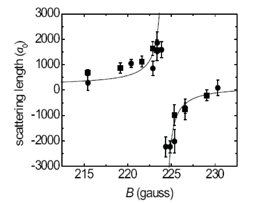
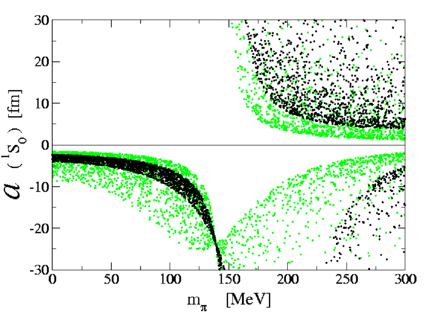
Figure 6: The left panel shows the scattering length of ⁴⁰K Atoms as a function of the magnetic field near a Feshbach resonance, from Regal (2005). The right panel shows the nucleon-nucleon scattering length in the ${}^{1}S_{0}$ channel as a function of the pion mass. The scatter plot indicates the uncertainty due to higher order terms in the chiral effective lagrangian. Figure from Beane & Savage (2003).

A dilute gas of fermions in the unitarity limit is a strongly coupled quantum liquid that exhibits many interesting properties. One interesting feature is universality. We are interested in the limit $(k_{F}a)\to\infty$ and $(k_{F}r)\to 0$, where $k_{F}$ is the Fermi momentum, $a$ is the scattering length and $r$ is the effective range. From dimensional analysis it is clear that the energy per particle at zero temperature has to be proportional to energy per particle of a free Fermi gas at the same density

$$\frac{E}{A}=\xi\Big{(}\frac{E}{A}\Big{)}_{0}=\xi\frac{3}{5}\Big{(}\frac{k_{F}^{2}}{2m}\Big{)}.$$ (76)

The constant $\xi$ is universal, i. e.  independent of the details of the system. Similar universal constants govern the magnitude of the gap in units of the Fermi energy and the equation of state at finite temperature.

Universal behavior in the unitarity limit is relevant to the physics of dilute neutron matter. The neutron-neutron scattering length is $a_{nn}=-18$ fm and the effective range is $r_{nn}=2.8$ fm. This means that there is a range of densities for which the inter-particle spacing is large compared to the effective range but small compared to the scattering length. It is interesting to note that the neutron scattering length depends on the quark masses in a way that is very similar to the dependence of atomic scattering lengths on the magnetic field near a Feshbach resonance Beane:2002xf , see Fig. 6.

4.1 Numerical Calculations

Figure 7: Lattice results for the energy per particle of a dilute Fermi gas from Lee & Schäfer (2005). We show the energy per particle in units of $3E_{F}/5$ as a function of temperature in units of $T_{F}$.

The calculation of the dimensionless quantity $\xi$ is a non-perturbative problem. In this section we shall tackle this problem using a combination of effective field theory and lattice field theory methods. We will study an analytical approach in the next section. We first observe that in the low density limit the details of the interaction are not important. The physics of the unitarity limit is captured by an effective lagrangian of point-like fermions interacting via a short-range interaction. The lagrangian is

$${\cal L}=\psi^{\dagger}\left(i\partial_{0}+\frac{\vec{\nabla}^{2}}{2m}\right)\psi-\frac{C_{0}}{2}\left(\psi^{\dagger}\psi\right)^{2},$$ (77)

as in Equ. (1). The usual strategy for dealing with the four-fermion interaction is to use a Hubbard-Stratonovich transformation as in Sect. 3.1. The partition function can be written as Lee:2004qd

$$Z=\int DsDcDc^{\ast}\exp\left[-S\right],$$ (78)

where $s$ is the Hubbard-Stratonovich field and $c$ is a Grassmann field. $S$ is a discretized euclidean action

$$S = \sum_{\vec{n},i}\left[e^{-\hat{\mu}\alpha_{t}}c_{i}^{\ast}(\vec{n})c_{i}(\vec{n}+\hat{0})-e^{\sqrt{-C_{0}\alpha_{t}}s(\vec{n})+\frac{C_{0}\alpha_{t}}{2}}(1-6h)c_{i}^{\ast}(\vec{n})c_{i}(\vec{n})\right]$$ (79)

$$\hskip 8.5359pt\mbox{}-h\sum_{\vec{n},l_{s},i}\left[c_{i}^{\ast}(\vec{n})c_{i}(\vec{n}+\hat{l}_{s})+c_{i}^{\ast}(\vec{n})c_{i}(\vec{n}-\hat{l}_{s})\right]+\frac{1}{2}\sum_{\vec{n}}s^{2}(\vec{n}).$$

Here $i$ labels spin and $\vec{n}$ labels lattice sites. Spatial and temporal unit vectors are denoted by $\hat{l}_{s}$ and $\hat{0}$, respectively. The temporal and spatial lattice spacings are $b_{\tau}$ and $b$. The dimensionless chemical potential is given by $\hat{\mu}=\mu b_{\tau}$. We define $\alpha_{t}$ as the ratio of the temporal and spatial lattice spacings and $h=\alpha_{t}/(2\hat{m})$. Note that for $C_{0}<0$ the action is real and standard Monte Carlo simulations are possible.

The four-fermion coupling is fixed by computing the sum of all particle-particle bubbles as in Sect. 2.1 but with the elementary loop function regularized on the lattice. Schematically,

$$\frac{m}{4\pi a}=\frac{1}{C_{0}}+\frac{1}{2}\sum_{\vec{p}}\frac{1}{E_{\vec{p}}},$$ (80)

where the sum runs over discrete momenta on the lattice and $E_{\vec{p}}$ is the lattice dispersion relation. A detailed discussion of the lattice regularized scattering amplitude can be found in Chen:2003vy ; Beane:2003da ; Lee:2004qd . For a given scattering length $a$ the four-fermion coupling is a function of the lattice spacing. The continuum limit correspond to taking the temporal and spatial lattice spacings $b_{\tau}$, $b$ to zero

$$b_{\tau}\mu\to 0,\hskip 28.45274ptbn^{1/3}\to 0,$$ (81)

keeping $an^{1/3}$ fixed. Here, $\mu$ is the chemical potential and $n$ is the density. Numerical results in the unitarity limit are shown in Fig. 7. From these simulations we concluded that $\xi=(0.09-0.42)$. Lee performed canonical simulations at $T=0$ and obtained Lee:2005fk $\xi=0.25$. Green Function Monte Carlo calculations give Carlson:2003wm $\xi=0.44$, and finite temperature lattice simulations have been extrapolated to $T=0$ to yield similar results Bulgac:2005pj ; Burovski:2006 .

4.2 Epsilon Expansion

It is also desirable to find a systematic analytical approach to the dilute Fermi liquid in the unitarity limit. Various possibilities have been considered, such as an expansion in the number of fermion species Furnstahl:2002gt ; Nikolic:2006 or the number of spatial dimensions Steele:2000qt ; Schafer:2005kg . Nussinov & Nussinov observed that the fermion many body system in the unitarity limit reduces to a free Fermi gas near $d=2$ spatial dimensions, and to a free Bose gas near $d=4$ Nussinov:2004 . Their argument was based on the behavior of the two-body wave function as the binding energy goes to zero. For $d=2$ it is well known that the limit of zero binding energy corresponds to an arbitrarily weak potential. In $d=4$ the two-body wave function at $a=\infty$ has a $1/r^{2}$ behavior and the normalization is concentrated near the origin. This suggests the many body system is equivalent to a gas of non-interacting bosons.

A systematic expansion based on the observation of Nussinov & Nussinov was studied by Nishida and Son Nishida:2006br ; Nishida:2006eu . In this section we shall explain their approach. We begin by restating the argument of Nussinov & Nussinov in the effective field theory language. In dimensional regularization $a\to\infty$ corresponds to $C_{0}\to\infty$. The fermion-fermion scattering amplitude (see equ. 7) is given by

$${\cal A}(p_{0},\vec{p})=\left(\frac{4\pi}{m}\right)^{d/2}\left[\Gamma\left(1-\frac{d}{2}\right)\right]^{-1}\frac{i}{\left(-p_{0}+E_{p}/2-i\delta\right)^{\frac{d}{2}-1}}\;,$$ (82)

where $\delta\to 0+$. As a function of $d$ the Gamma function has poles at $d=2,4,\ldots$ and the scattering amplitude vanishes at these points. Near $d=2$ the scattering amplitude is energy and momentum independent. For $d=4-\epsilon$ we find

$${\cal A}(p_{0},\vec{p})=\frac{8\pi^{2}\epsilon}{m^{2}}\frac{i}{p_{0}-E_{p}/2+i\delta}+O(\epsilon^{2})\,.$$ (83)

We observe that at leading order in $\epsilon$ the scattering amplitude looks like the propagator of a boson with mass $2m$. The boson-fermion coupling is $g^{2}=(8\pi^{2}\epsilon)/m^{2}$ and vanishes as $\epsilon\to 0$. This suggests that we can set up a perturbative expansion involving fermions of mass $m$ weakly coupled to bosons of mass $2m$. In the unitarity limit the Hubbard-Stratonovich transformed lagrangian reads

$${\cal L}=\Psi^{\dagger}\left[i\partial_{0}+\sigma_{3}\frac{\vec{\nabla}^{2}}{2m}\right]\Psi+\mu\Psi^{\dagger}\sigma_{3}\Psi+\left(\Psi^{\dagger}\sigma_{+}\Psi\phi+h.c.\right)\ ,$$

where $\Psi=(\psi_{\uparrow},\psi_{\downarrow}^{\dagger})^{T}$ is a two-component Nambu-Gorkov field, $\sigma_{i}$ are Pauli matrices acting in the Nambu-Gorkov space and $\sigma_{\pm}=(\sigma_{1}\pm i\sigma_{2})/2$. In the superfluid phase $\phi$ acquires an expectation value. We write

$$\phi=\phi_{0}+g\varphi,\hskip 28.45274ptg=\frac{\sqrt{8\pi^{2}\epsilon}}{m}\left(\frac{m\phi_{0}}{2\pi}\right)^{\epsilon/4},$$ (84)

where $\phi_{0}=\langle\phi\rangle$. The scale $M^{2}=m\phi_{0}/(2\pi)$ was introduced in order to have a correctly normalized boson field. The scale parameter is arbitrary, but this particular choice simplifies some of the loop integrals. In order to get a well defined perturbative expansion we add and subtract a kinetic term for the boson field to the lagrangian. We include the kinetic term in the free part of the lagrangian

$${\cal L}_{0}=\Psi^{\dagger}\left[i\partial_{0}+\sigma_{3}\frac{\vec{\nabla}^{2}}{2m}+\phi_{0}(\sigma_{+}+\sigma_{-})\right]\Psi+\varphi^{\dagger}\left(i\partial_{0}+\frac{\vec{\nabla}^{2}}{4m}\right)\varphi\,.$$ (85)

The interacting part is

$${\cal L}_{I}=g\left(\Psi^{\dagger}\sigma_{+}\Psi\varphi+h.c\right)+\mu\Psi^{\dagger}\sigma_{3}\Psi-\varphi^{\dagger}\left(i\partial_{0}+\frac{\vec{\nabla}^{2}}{4m}\right)\varphi\,.$$ (86)

Note that the interacting part generates self energy corrections to the boson propagator which, by virtue of equ. (83), cancel against the kinetic term of boson field. We have also included the chemical potential term in ${\cal L}_{I}$. This is motivated by the fact that near $d=4$ the system reduces to a non-interacting Bose gas and $\mu\to 0$. We will count $\mu$ as a quantity of $O(\epsilon)$.

The Feynman rules are quite simple. The fermion and boson propagators are

$$G(p_{0},\vec{p}) = \frac{i}{p_{0}^{2}-E_{\vec{p}}^{2}-\phi_{0}^{2}}\left[\begin{array}[]{cc}p_{0}+E_{\vec{p}}&-\phi_{0}\\ -\phi_{0}&p_{0}-E_{\vec{p}}\end{array}\right]\ ,$$ (89)

$$D(p_{0},\vec{p}) = \frac{i}{p_{0}-E_{\vec{p}}/2}\ ,$$ (90)

and the fermion-boson vertices are $ig\sigma^{\pm}$. Insertions of the chemical potential are $i\mu\sigma_{3}$. Both $g^{2}$ and $\mu$ are corrections of order $\epsilon$. In order to verify that the $\epsilon$ expansion is well defined we have to check that higher order diagrams do not generate powers of $1/\epsilon$. Studying the superficial degree of divergence of diagrams involving the propagators given in equ. (89) one can show that there is only a finite number of one-loop diagrams that generate $1/\epsilon$ terms.

Figure 8: Leading order contributions to the effective potential in the $\epsilon$ expansion. Solid lines are fermion propagators, dashed lines are boson propagators, and the cross is an insertion of the chemical potential.

The leading order diagrams that contribute to the effective potential are shown in Fig. 8. The first diagram is the free fermion loop which is $O(1)$. The second diagram is the $\mu$ insertion which is $O(1)$ because the loop diagram is divergent in $d=4$. The two-loop diagram is $O(\epsilon)$ because of the factor of $g^{2}$ from the vertices. The free fermion loop diagram is

$$V_{0}=i\int\frac{dp_{0}}{2\pi}\int\frac{d^{d}p}{(2\pi)^{d}}\log\left[p_{0}^{2}-E_{\vec{p}}^{2}-\phi_{0}^{2}\right]=-\int\frac{d^{d}p}{(2\pi)^{d}}\,\sqrt{E^{2}_{\vec{p}}+\phi_{0}^{2}}\ .$$ (91)

The integral can be computed analytically. Expanding to first order in $\epsilon=4-d$ we get

$$V_{0}=\frac{\phi_{0}}{3}\left[1+\frac{7-3(\gamma+\log(2))}{6}\,\epsilon\right]\left(\frac{m\phi_{0}}{2\pi}\right)^{d/2}.$$ (92)

The $\mu$ insertion is given by

$$V_{1}=\mu\int\frac{d^{d}p}{(2\pi)^{d}}\frac{E_{\vec{p}}}{\sqrt{E^{2}_{\vec{p}}+\phi_{0}^{2}}}.$$ (93)

Again, the integral can be computed analytically. The result is

$$V_{1}=-\frac{\mu}{\epsilon}\left[1+\frac{1-2(\gamma-\log(2))}{4}\,\epsilon\right]\left(\frac{m\phi_{0}}{2\pi}\right)^{d/2}$$ (94)

Nishida and Son also computed the two-loop contribution shown in Fig. 8. The result is

$$V_{2}=-C\epsilon\left(\frac{m\phi_{0}}{2\pi}\right)^{d/2},$$ (95)

where $C\simeq 0.14424$. We can now determine the minimum of the effective potential. We find

$$\phi_{0}=\frac{2\mu}{\epsilon}\,\left[1+(3C-1+\log(2))\,\epsilon+O(\epsilon^{2})\right].$$ (96)

The value of $V=V_{0}+V_{1}+V_{2}$ at $\phi_{0}$ determines the pressure and $n=\partial P/\partial\mu$ gives the density. We find

$$n=\frac{1}{\epsilon}\,\left[1-\frac{1}{4}\left(2\gamma-1-\log(2)\right)+O(\epsilon^{2})\right]\left(\frac{m\phi_{0}}{2\pi}\right)^{d/2}.$$ (97)

For comparison, the density of a free Fermi gas in $d$ dimensions is

$$n=\frac{2}{(4\pi)^{d/2}}\frac{k_{F}^{d}}{\Gamma\left(1+\frac{d}{2}\right)}.$$ (98)

This equation determines the relation between $\epsilon_{F}\equiv k_{F}^{2}/(2m)$ and the density. We get

$$\epsilon_{F}=\frac{2\pi}{m}\left[\frac{n}{2}\Gamma\left(\frac{d}{2}+1\right)\right]^{2/d}.$$ (99)

We determine $\epsilon_{F}$ for the interacting gas by inserting $n$ from equ. (97) into equ. (99). The universal parameter is $\xi=\mu/\epsilon_{F}$ . We find

$$\xi=\frac{1}{2}\epsilon^{3/2}+\frac{1}{16}\epsilon^{5/2}\log(\epsilon)-0.025\epsilon^{5/2}+\ldots=0.475\hskip 7.11317pt(\epsilon=1),$$ (100)

which agrees quite well with the result of fixed node quantum Monte Carlo calculations. The calculation has been extended to $O(\epsilon^{7/2})$ by Arnold et al. Arnold:2006fr . Unfortunately, the next term is very large and it appears necessary to combine the expansion in $4-\epsilon$ dimensions with a $2+\epsilon$ expansion in order to extract useful results. The $\epsilon$ expansion has also been applied to the calculation of the gap Nishida:2006br , the critical temperature Nishida:2006rp and the critical chemical potential imbalance Rupak:2006et ; Nishida:2006eu .

5 QCD and its symmetries

5.1 Introduction

Before we discuss QCD at large baryon density we would like to provide a quick review of QCD and the symmetries of QCD. The elementary degrees of freedom are quark fields $\psi^{a}_{\alpha,f}$ and gluons $A_{\mu}^{a}$. Here, $a$ is color index that transforms in the fundamental representation for fermions and in the adjoint representation for gluons. Also, $f$ labels the quark flavors $u,d,s,c,b,t$. In practice, we will focus on the three light flavors up, down and strange. The QCD lagrangian is

$${\cal L}=\sum_{f}^{N_{f}}\bar{\psi}_{f}(iD/\,-m_{f})\psi_{f}-\frac{1}{4}G_{\mu\nu}^{a}G_{\mu\nu}^{a},$$ (101)

where the field strength tensor is defined by

$$G_{\mu\nu}^{a}=\partial_{\mu}A_{\nu}^{a}-\partial_{\nu}A_{\mu}^{a}+gf^{abc}A_{\mu}^{b}A_{\nu}^{c},$$ (102)

and the covariant derivative acting on quark fields is

$$iD/\,\psi=\gamma^{\mu}\left(i\partial_{\mu}+gA_{\mu}^{a}\frac{\lambda^{a}}{2}\right)\psi.$$ (103)

QCD has a number of remarkable properties. Most remarkably, even though QCD accounts for the rich phenomenology of hadronic and nuclear physics, it is an essentially parameter free theory. To first approximation, the masses of the light quarks $u,d,s$ are too small to be important, while the masses of the heavy quarks $c,b,t$ are too heavy. If we set the masses of the light quarks to zero and take the masses of the heavy quarks to be infinite then the only parameter in the QCD lagrangian is the coupling constant, $g$. Once quantum corrections are taken into account $g$ becomes a function of the scale at which it is measured. If the scale is large then the coupling is small, but in the infrared the coupling becomes large. This is the famous phenomenon of asymptotic freedom. Since the coupling depends on the scale the dimensionless parameter $g$ is traded for a dimensionful scale parameter $\Lambda_{QCD}$. Since $\Lambda_{QCD}$ is the only dimensionful quantity in QCD with massless fermions it is not really a parameter of QCD, but reflects our choice of units. In standard units, $\Lambda_{QCD}\simeq 200\,{\rm MeV}\simeq 1\,{\rm fm}^{-1}$.

Another important feature of the QCD lagrangian are its symmetries. First of all, the lagrangian is invariant under local gauge transformations $U(x)\in SU(3)_{c}$

$$\psi(x)\to U(x)\psi(x),\hskip 28.45274ptA_{\mu}(x)\to U(x)A_{\mu}U^{\dagger}(x)+iU(x)\partial_{\mu}U^{\dagger}(x),$$ (104)

where $A_{\mu}=A_{\mu}^{a}(\lambda^{a}/2)$. In the QCD ground state at zero temperature and density the local color symmetry is confined. This implies that all excitations are singlets under the gauge group.

The dynamics of QCD is completely independent of flavor. This implies that if the masses of the quarks are equal, $m_{u}=m_{d}=m_{s}$, then the theory is invariant under arbitrary flavor rotations of the quark fields

$$\psi_{f}\to V_{fg}\psi_{g},$$ (105)

where $V\in SU(3)$. This is the well known flavor (isospin) symmetry of the strong interactions. If the quark masses are not just equal, but equal to zero, then the flavor symmetry is enlarged. This can be seen by defining left and right-handed fields

$$\psi_{L,R}=\frac{1}{2}(1\pm\gamma_{5})\psi.$$ (106)

In terms of $L/R$ fields the fermionic lagrangian is

$${\cal L}=\bar{\psi}_{L}(iD/\,)\psi_{L}+\bar{\psi}_{R}(iD/\,)\psi_{R}+\bar{\psi}_{L}M\psi_{R}+\bar{\psi}_{R}M\psi_{L},$$ (107)

where $M={\rm diag}(m_{u},m_{d},m_{s})$. We observe that if quarks are massless, $m_{u}=m_{d}=m_{s}=0$, then there is no coupling between left and right handed fields. As a consequence, the lagrangian is invariant under independent flavor transformations of the left and right handed fields.

$$\psi_{L,f}\to L_{fg}\psi_{L,g},\hskip 28.45274pt\psi_{R,f}\to R_{fg}\psi_{R,g},$$ (108)

where $(L,R)\in SU(3)_{L}\times SU(3)_{R}$. In the real world, of course, the masses of the up, down and strange quarks are not zero. Nevertheless, since $m_{u},m_{d}\ll m_{s}<\Lambda_{QCD}$ QCD has an approximate chiral symmetry.

In the QCD ground state at zero temperature and density the flavor symmetry is realized, but the chiral symmetry is spontaneously broken by a quark-anti-quark condensate $\langle\bar{\psi}_{L}\psi_{R}+\bar{\psi}_{R}\psi_{L}\rangle$. As a result, the observed hadrons can be approximately assigned to representations of the $SU(3)_{V}$ flavor group, but not to representations of $SU(3)_{L}\times SU(3)_{R}$. Nevertheless, chiral symmetry has important implications for the dynamics of QCD at low energy. Goldstone’s theorem implies that the breaking of $SU(3)_{L}\times SU(3)_{R}\to SU(3)_{V}$ is associated with the appearance of an octet of (approximately) massless pseudoscalar Goldstone bosons. Chiral symmetry places important restrictions on the interaction of the Goldstone bosons. These constraints are obtained most easily from the low energy effective chiral lagrangian. At leading order we have

$${\cal L}=\frac{f_{\pi}^{2}}{4}{\rm Tr}\left[\partial_{\mu}\Sigma\partial^{\mu}\Sigma^{\dagger}\right]+\Big{[}B{\rm Tr}(M\Sigma^{\dagger})+h.c.\Big{]}+\ldots,$$ (109)

where $\Sigma=\exp(i\phi^{a}\lambda^{a}/f_{\pi})$ is the chiral field, $f_{\pi}$ is the pion decay constant and $M$ is the mass matrix. Expanding $\Sigma$ in powers of the pion, kaon and eta fields $\phi^{a}$ we can derive the leading order chiral perturbation theory results for Goldstone boson scattering and the coupling of Goldstone bosons to external fields. Higher order corrections originate from loops and higher order terms in the effective lagrangian.

Finally, we observe that the QCD lagrangian has two $U(1)$ symmetries,

$$U(1)_{B}:\hskip 28.45274pt \psi_{L}\to e^{i\phi}\psi_{L},\hskip 28.45274pt \psi_{R}\to e^{i\phi}\psi_{R}$$ (110)

$$U(1)_{A}:\hskip 28.45274pt \psi_{L}\to e^{i\alpha}\psi_{L},\hskip 28.45274pt \psi_{R}\to e^{-i\alpha}\psi_{R}.$$ (111)

The $U(1)_{B}$ symmetry is exact even if the quarks are not massless. Superficially, it appears that the $U(1)_{A}$ symmetry is explicitly broken by the quark masses and spontaneously broken by the quark condensate. However, there is no Goldstone boson associated with spontaneous $U(1)_{A}$ breaking. The reason is that at the quantum level the $U(1)_{A}$ symmetry is broken by an anomaly. The divergence of the $U(1)_{A}$ current is given by

$$\partial^{\mu}j_{\mu}^{5}=\frac{N_{f}g^{2}}{16\pi^{2}}G^{a}_{\mu\nu}\tilde{G}^{a}_{\mu\nu},$$ (112)

where $\tilde{G}^{a}_{\mu\nu}=\epsilon_{\mu\nu\alpha\beta}G^{a}_{\alpha\beta}/2$ is the dual field strength tensor.

5.2 QCD at finite density

In the real world the quark masses are not equal and the only exact global symmetries of QCD are the $U(1)_{f}$ flavor symmetries associated with the conservation of the number of up, down, and strange quarks. If we take into account the weak interactions then flavor is no longer conserved and the only exact symmetries are the $U(1)_{B}$ of baryon number and the $U(1)_{Q}$ of electric charge.

In the following we study hadronic matter at non-zero baryon density. We will mostly focus on systems at non-zero baryon chemical potential but zero electron $U(1)_{Q}$ chemical potential. We should note that in the context of neutron stars we are interested in situations when the electric charge, but not necessarily the electron chemical potential, is zero. Also, if the system is in equilibrium with respect to strong, but not to weak interactions, then non-zero flavor chemical potentials may come into play.

The partition function of QCD at non-zero baryon chemical potential is given by

$$Z=\sum_{i}\exp\left(-\frac{E_{i}-\mu N_{i}}{T}\right),$$ (113)

where $i$ labels all quantum states of the system, $E_{i}$ and $N_{i}$ are the energy and baryon number of the state $i$. If the temperature and chemical potential are both zero then only the ground state contributes to the partition function. All other states give contributions that are exponentially small if the volume of the system is taken to infinity. In QCD there is a mass gap for states that carry baryon number. As a consequence there is an onset chemical potential

$$\mu_{c}=\min_{i}(E_{i}/N_{i}),$$ (114)

such that the partition function is independent of $\mu$ for $\mu<\mu_{c}$. For $\mu>\mu_{c}$ the baryon density is non-zero. If the chemical potential is just above the onset chemical potential we can describe QCD, to first approximation, as a dilute gas of non-interacting nucleons. In this approximation $\mu_{c}=m_{N}$. Of course, the interaction between nucleons cannot be neglected. Without it, we would not have stable nuclei. As a consequence, nuclear matter is self-bound and the energy per baryon in the ground state is given by

$$\frac{E_{N}}{N}-m_{N}\simeq-15\,{\rm MeV}.$$ (115)

The onset transition is a first order transition at which the baryon density jumps from zero to nuclear matter saturation density, $\rho_{0}\simeq 0.14\,{\rm fm}^{-3}$. The first order transition continues into the finite temperature plane and ends at a critical endpoint at $T=T_{c}\simeq 10$ MeV, see Fig. 9.

Figure 9: Schematic phase diagram of hadronic matter as a function of the baryon and electron chemical potentials and temperature.

Nuclear matter is a complicated many-body system and, unlike the situation at zero density and finite temperature, there is little information from numerical simulations on the lattice. This is related to the so-called ’sign problem’. At non-zero chemical potential the euclidean fermion determinant is complex and standard Monte-Carlo techniques based on importance sampling fail. Recently, some progress has been made in simulating QCD for small $\mu$ and $T\simeq T_{c}$ Fodor:2001pe ; deForcrand:2002ci ; Allton:2002zi , but the regime of small temperature remains inaccessible.

In neutron stars there is a non-zero electron chemical potential and matter is neutron rich. Pure neutron matter has positive pressure and is stable at arbitrarily low density. As we emphasized in Sect. 4 dilute neutron matter has universal properties that can be explored using atomic systems. As the density increases three and four-body interactions as well as short range forces become more important and effective field theory methods are no longer applicable.

If the density is much larger than nuclear matter saturation density, $\rho\gg\rho_{0}$, we expect the problem to simplify. In this regime it is natural to use a system of non-interacting quarks as a starting point Collins:1974ky . The low energy degrees of freedom are quark excitations and holes in the vicinity of the Fermi surface. Since the Fermi momentum is large, asymptotic freedom implies that the interaction between quasi-particles is weak. We shall see that this does not imply that the phase diagram is simple, but it does imply that the phase structure can be studied in a systematic fashion.

6 Effective field theory near the Fermi surface

6.1 High density effective theory

The QCD Lagrangian in the presence of a chemical potential is given by

$${\mathcal{L}}=\bar{\psi}\left(iD/\,+\mu\gamma_{0}-M\right)\psi-\frac{1}{4}G^{a}_{\mu\nu}G^{a}_{\mu\nu},$$ (116)

where $D_{\mu}=\partial_{\mu}+igA_{\mu}$ is the covariant derivative, $M$ is the mass matrix and $\mu$ is the baryon chemical potential. If the baryon chemical potential is large, $\mu\gg\Lambda_{QCD}$, then we expect the effective coupling to be small and weak coupling methods to be applicable. We shall see, however, that the weak coupling expansion is not a simple expansion in the number of loops. Effective field theory methods are useful in constructing a systematic weak coupling expansion.

The main observation is that the relevant low energy degrees of freedom are particle and hole excitations in the vicinity of the Fermi surface. We shall describe these excitations in terms of the field $\psi_{v}(x)$, where $v$ is the Fermi velocity. At tree level, the quark field $\psi$ can be decomposed as $\psi=\psi_{v,+}+\psi_{v,-}$ where $\psi_{v,\pm}=P_{v,\pm}\psi$ with $P_{v,\pm}=\frac{1}{2}(1\pm\vec{\alpha}\cdot\hat{v})\psi$. Note that $P_{v,\pm}$ is a projector on states with positive/negative energy. To leading order in $1/\mu$ we can eliminate the field $\psi_{-}$ using its equation of motion. The lagrangian for the $\psi_{+}$ field is given by Hong:2000tn ; Hong:2000ru ; Nardulli:2002ma

$${\cal L}=\psi_{v}^{\dagger}\left(iv\cdot D-\frac{D_{\perp}^{2}}{2\mu}-\frac{g\sigma_{\mu\nu}G_{\perp}^{\mu\nu}}{4\mu}+\ldots\right)\psi_{v}-\frac{1}{4}G^{a}_{\mu\nu}G^{a}_{\mu\nu}+\ldots.$$ (117)

with $v_{\mu}=(1,\vec{v})$. Note that $v$ labels patches on the Fermi surface, and that the number of these patches grows as $\mu^{2}$. The leading order $v\cdot D$ interaction does not connect quarks with different $v$, but soft gluons can be exchanged between quarks in different patches. In addition to that, there are four, six, etc. fermion operators that contain fermion fields with different velocity labels. These operators are constrained by the condition that the sum of the velocities has to be zero.

Figure 10: Kinematics of four-fermion operators in the effective theory.

In the case of four-fermion operators there are two kinds of interactions that satisfy this constraint, see Fig. 10. The first possibility is that both the incoming and outgoing fermion momenta are back-to-back. This corresponds to the BCS interaction

$${\cal L}=\frac{1}{\mu^{2}}\sum_{v^{\prime},\Gamma,\Gamma^{\prime}}V_{l}^{\Gamma\Gamma^{\prime}}R_{l}^{\Gamma\Gamma^{\prime}}(\vec{v}\cdot\vec{v}^{\prime})\Big{(}\psi_{v}\Gamma\psi_{-v}\Big{)}\Big{(}\psi^{\dagger}_{v^{\prime}}\Gamma^{\prime}\psi^{\dagger}_{-v^{\prime}}\Big{)},$$ (118)

where $\vec{v}\cdot\vec{v}^{\prime}=\cos\theta$ is the scattering angle, $R_{l}^{\Gamma\Gamma^{\prime}}(x)$ is a set of orthogonal polynomials, and $\Gamma,\Gamma^{\prime}$ determine the color, flavor and spin structure. The second possibility is that the final momenta are equal to the initial momenta up to a rotation around the axis defined by the sum of the incoming momenta. The relevant four-fermion operator is

$${\cal L}=\frac{1}{\mu^{2}}\sum_{v^{\prime},\Gamma,\Gamma^{\prime}}F_{l}^{\Gamma\Gamma^{\prime}}R_{l}^{\Gamma\Gamma^{\prime}}(\vec{v}\cdot\vec{v}^{\prime})\Big{(}\psi_{v}\Gamma\psi_{v^{\prime}}\Big{)}\Big{(}\psi^{\dagger}_{\tilde{v}}\Gamma^{\prime}\psi^{\dagger}_{\tilde{v}^{\prime}}\Big{)}.$$ (119)

In a system with short range interactions only the quantities $F_{l}(0)$ are known as Fermi liquid parameters.

6.2 Hard Loops

The effective field theory expansion is complicated by the fact that the number of patches $N_{v}\sim\mu^{2}/\Lambda^{2}$ grows with the chemical potential. This implies that some higher order contributions that are suppressed by $1/\mu^{2}$ can be enhanced by powers of $N_{v}$. The natural solution to this problem is to sum the leading order diagrams in the large $N_{v}$ limit Schafer:2004zf . For gluon $n$-point functions this corresponds to the well known hard dense loop approximation Braaten:1989mz ; Blaizot:1993bb ; Manuel:1995td .

Figure 11: Hard dense loop contribution to gluon $n$-point functions.

The simplest example is the gluon two point function. At leading order in $g$ and $1/\mu$ we have

$$\Pi^{ab}_{\mu\nu}(p)=2g^{2}N_{f}\frac{\delta^{ab}}{2}\sum_{\vec{v}}v_{\mu}v_{\nu}\int\frac{d^{4}k}{(2\pi)^{4}}\frac{1}{(k_{0}-l_{k})(k_{0}+p_{0}-l_{k+p})},$$ (120)

where $l_{k}=\vec{v}\cdot\vec{k}$. We note that taking the momentum of the external gluon to zero automatically selects forward scattering. We also observe that the gluon can interact with fermions of any Fermi velocity so that the polarization function involves a sum over all patches. After performing the $k_{0}$ integration we get

$$\Pi^{ab}_{\mu\nu}(p)=2g^{2}N_{f}\frac{\delta^{ab}}{2}\sum_{\vec{v}}v_{\mu}v_{\nu}\int\frac{d^{2}l_{\perp}}{(2\pi)^{2}}\int\frac{dl_{k}}{2\pi}\frac{l_{p}}{p_{0}-l_{p}}\frac{\partial n_{k}}{\partial l_{k}},$$ (121)

where $n_{k}$ is the Fermi distribution function. We note that the $l_{k}$ integration is automatically restricted to small momenta. The integral over the transverse momenta $l_{\perp}$, on the other hand, diverges quadratically with the cutoff $\Lambda_{\perp}$. We observe, however, that the sum over patches and the integral over $l_{\perp}$ can be combined into an integral over the entire Fermi surface

$$\frac{1}{2\pi}\sum_{\vec{v}}\int\frac{d^{2}l_{\perp}}{(2\pi)^{2}}=\frac{\mu^{2}}{2\pi^{2}}\int\frac{d\Omega}{4\pi}.$$ (122)

This means that the transverse momentum integral is extended all the way up to $\mu$. Because the energy of the fermions is small but the loop momentum is large the integral is referred to as a hard dense loop. We find

$$\Pi^{ab}_{\mu\nu}(p)=2m^{2}\delta^{ab}\int\frac{d\Omega}{4\pi}v_{\mu}v_{\nu}\left\{1-\frac{p_{0}}{p_{0}-l_{p}}\right\},$$ (123)

where we have defined the effective gluon mass $m^{2}=N_{F}g^{2}\mu^{2}/(4\pi^{2})$. This result has the same structure as the non-relativistic expression given in equ. (32), but the tadpole contribution is missing. As a consequence, equ. (123) is not transverse. In the relativistic theory the tadpole contribution originates from the $D_{\perp}^{2}/(2\mu)$ in the effective lagrangian. The tadpole is proportional to the total density and corresponds to a counterterm Hong:2000tn

$${\cal L}=\frac{1}{2}m^{2}\int\frac{d\Omega}{4\pi}(\vec{A}_{\perp})^{2}.$$ (124)

Putting everything together we find

$$\Pi^{ab}_{\mu\nu}(p)=2m^{2}\delta^{ab}\int\frac{d\Omega}{4\pi}\left\{\delta_{\mu 0}\delta_{\nu 0}-\frac{v_{\mu}v_{\nu}p_{0}}{p_{0}-l_{p}}\right\}.$$ (125)

The gluonic three-point function shown in Fig. 11b can be computed in the same fashion. We find

$$\Gamma^{abc}_{\mu\nu\alpha}(p,q,r)=igf^{abc}2m^{2}\int\frac{d\Omega}{4\pi}v_{\mu}v_{\alpha}v_{\beta}\left\{\frac{q_{0}}{(q\cdot v)(p\cdot v)}-\frac{r_{0}}{(r\cdot v)(p\cdot v)}\right\},$$ (126)

where $p,q,r$ are the incoming gluon momenta ($p+q+r=0$). We note that in the case of the three point function, as well as in all higher $n$-point functions, there are no tadpole or counterterm contributions. There is a simple generating functional for these loop integrals which is known as the hard dense loop (HDL) effective action Braaten:1991gm

$${\cal L}_{HDL}=-\frac{m^{2}}{2}\sum_{v}\,G^{a}_{\mu\alpha}\frac{v^{\alpha}v^{\beta}}{(v\cdot D)^{2}}G^{a}_{\mu\beta}.$$ (127)

This is a gauge invariant, but non-local, effective lagrangian.

6.3 Non-Fermi liquid effective field theory

In this Section we shall study the effective field theory in the regime $\omega<m$ where $\omega$ is the excitation energy and $m$ is the effective gluon mass Schafer:2005mc . In the previous section we argued that hard dense loops have to be resummed in order to obtain a consistent low energy expansion. The effective lagrangian is given by

$${\cal L}=\psi_{v}^{\dagger}\left(iv\cdot D-\frac{D_{\perp}^{2}}{2\mu}\right)\psi_{v}-\frac{1}{4}G^{a}_{\mu\nu}G^{a}_{\mu\nu}+{\cal L}_{HDL}+{\cal L}_{4f}+\ldots\,.$$ (128)

Since electric fields are screened the interaction at low energies is dominated by the exchange of magnetic gluons. The transverse gauge boson propagator is

$$D_{ij}(k)=-\frac{i(\delta_{ij}-\hat{k}_{i}\hat{k}_{j})}{k_{0}^{2}-\vec{k}^{2}+i\frac{\pi}{2}m^{2}\frac{k_{0}}{|\vec{k}|}},$$ (129)

where we have assumed that $|k_{0}|<|\vec{k}|$. We observe that the propagator becomes large in the regime $|k_{0}|\sim|\vec{k}|^{3}/m^{2}$. If the energy is small, $|k_{0}|\ll m$, then the typical energy is much smaller than the typical momentum,

$$|\vec{k}|\sim(m^{2}|k_{0}|)^{1/3}\gg|k_{0}|.$$ (130)

This implies that the gluon is very far off its energy shell and not a propagating state. We can compute loop diagrams containing quarks and transverse gluons by picking up the pole in the quark propagator, and then integrate over the cut in the gluon propagator using the kinematics dictated by equ. (130). In order for a quark to absorb the large momentum carried by a gluon and stay close to the Fermi surface the gluon momentum has to be transverse to the momentum of the quark. This means that the term $k_{\perp}^{2}/(2\mu)$ in the quark propagator is relevant and has to be kept at leading order. Equation (130) shows that $k_{\perp}^{2}/(2\mu)\gg k_{0}$ as $k_{0}\to 0$. This means that the pole of the quark propagator is governed by the condition $k_{||}\sim k_{\perp}^{2}/(2\mu)$. We find

$$k_{\perp}\sim g^{2/3}\mu^{2/3}k_{0}^{1/3},\hskip 14.22636ptk_{||}\sim g^{4/3}\mu^{1/3}k_{0}^{2/3}.$$ (131)

In the low energy regime propagators and vertices can be simplified even further. The quark and gluon propagators are

$$S_{\alpha\beta}(p)=\frac{i\delta_{\alpha\beta}}{p_{0}-p_{||}-\frac{p_{\perp}^{2}}{2\mu}+i\epsilon{\it sgn}(p_{0})},$$ (132)

$$D_{ij}(k)=\frac{i\delta_{ij}}{k_{\perp}^{2}-i\frac{\pi}{2}m^{2}\frac{k_{0}}{k_{\perp}}},$$ (133)

and the quark gluon vertex is $gv_{i}(\lambda^{a}/2)$. Higher order corrections can be found by expanding the quark and gluon propagators as well as the HDL vertices in powers of the small parameter $\epsilon\equiv(k_{0}/m)$.

Figure 12: One-loop contributions to the quark self energy and the quark-gluon vertex. The black blob in the third diagram denotes the HDL gluon three point function. In the magnetic regime the graphs scale as $\omega\log(\omega)$, $\omega^{1/3}$ and $\omega^{2/3}$, respectively.

The regime in which all momenta, including external ones, satisfy the scaling relation (131) is completely perturbative, i.e. graphs with extra loops are always suppressed by extra powers of $\epsilon^{1/3}$. One way to see this is to rescale the fields in the effective lagrangian so that the kinetic terms are scale invariant under the transformation $(x_{0},x_{||},x_{\perp})$ $\to$ $(\epsilon^{-1}x_{0},\epsilon^{-2/3}x_{||},\epsilon^{-1/3}x_{\perp})$. The scaling behavior of the fields is $\psi\to\epsilon^{5/6}\psi$ and $A_{i}\to\epsilon^{5/6}A_{i}$. We find that the scaling dimension of all interaction terms is positive. The quark gluon vertex scales as $\epsilon^{1/6}$, the HDL three gluon vertex scales as $\epsilon^{1/2}$, and the four gluon vertex scales as $\epsilon$. Since higher order diagrams involve at least one pair of quark gluon vertices the expansion involves positive powers of $\epsilon^{1/3}$.

As a simple example we consider the fermion self energy in the limit $p_{0}\to 0$. The one-loop diagram is

$$\Sigma(p) = -ig^{2}C_{F}\int\frac{dk_{0}}{2\pi}\int\frac{dk_{\perp}^{2}}{(2\pi)^{2}}\ \frac{k_{\perp}}{k_{\perp}^{3}+i\eta k_{0}}$$ (134)

$$\hskip 14.22636pt\mbox{}\times\int\frac{dk_{||}}{2\pi}\ \frac{\Theta(p_{0}+k_{0})}{k_{||}+p_{||}-(k_{\perp}+p_{\perp})^{2}/(2\mu)+i\epsilon},$$

with $C_{F}=(N_{c}^{2}-1)/(2N_{c})$ and $\eta=(\pi/2)m^{2}$. This expression shows a number of interesting features. First we observe that the longitudinal and transverse momentum integrations factorize. The longitudinal momentum integral can be performed by picking up the pole in the quark propagator. The result is independent of the external momenta and only depends on the external energy. The transverse momentum integral is logarithmically divergent. We find Vanderheyden:1996bw ; Manuel:2000mk ; Brown:2000eh ; Boyanovsky:2000bc ; Ipp:2003cj

$$\Sigma(p)=\frac{g^{2}}{9\pi^{2}}p_{0}\log\left(\frac{\Lambda}{|p_{0}|}\right),$$ (135)

where $\Lambda$ is a cutoff for the $k_{\perp}$ integral. We showed that the logarithmic divergence can be absorbed in the parameters of the effective theory Schafer:2004zf . In order to fix the corresponding counterterm we have include electric gluon exchanges For $k_{0}\ll m$ the electric gluon propagator is given by

$$D_{00}(k)=-\frac{i}{\vec{k}^{2}+2m^{2}}.$$ (136)

Higher order corrections can be obtained by expanding the full HDL expression in powers of $k_{0}/m$. The electric contribution is dominated by large momenta and does not contribute to fractional powers or logarithms of $k_{0}$. We get

$$\Sigma(p) = ig^{2}C_{F}\int\frac{dk_{0}}{2\pi}\int\frac{dk_{\perp}^{2}}{(2\pi)^{2}}\ \frac{1}{k_{\perp}^{2}+2m^{2}}$$ (137)

$$\hskip 14.22636pt\mbox{}\times\int\frac{dk_{||}}{2\pi}\ \frac{\Theta(p_{0}+k_{0})}{k_{||}+p_{||}-(k_{\perp}+p_{\perp})^{2}/(2\mu)+i\epsilon}.$$

This contribution scales as $p_{0}\log(\Lambda/m)$. The logarithm of the cutoff cancels the logarithm in equ. (135). We get Ipp:2003cj

$$\Sigma(p_{0})=\frac{g^{2}}{9\pi^{2}}\left[p_{0}\log\left(\frac{4\sqrt{2}m}{\pi|p_{0}|}\right)+p_{0}+i\frac{\pi}{2}|p_{0}|\right].$$ (138)

Finally, there are contributions from the hard regime in which both the energy and the momentum of the gluon are large, $k_{0}\sim|\vec{k}|\geq m$. This regime corresponds to the HDL term in the fermion self energy Manuel:1995td ; Schafer:2003jn . The HDL term gives an $O(g^{2})$ correction to the low energy parameters $v_{F}$ and $\delta\mu$.

The logarithmic term in the fermion self energy leads to a breakdown of Fermi liquid theory. The quasi-particle velocity

$$v(p_{0})=\frac{1}{1+\Sigma^{\prime}(p_{0})}$$ (139)

and the wave function renormalization go to zero logarithmically as the quasi-particle energy goes to zero. One physical consequence of this behavior is an anomalous $T\log(T)$ term in the specific heat Holstein:1973 ; Ipp:2003cj . The effective theory can also be used to study perturbative corrections in other quantities. We find, in particular, a QCD version of Migdal’s theorem. Migdal showed that vertex corrections to the electron-phonon coupling are suppressed by the ratio of the electron mass to the mass of the positive ions Abrikosov:1963 . In the Landau damping regime of QCD loop corrections to the quark-gluon vertex are suppressed by powers of $\epsilon^{1/3}$.

6.4 Color superconductivity

In Sect. (3.1) we showed that the particle-particle scattering amplitude in the BCS channel $q(\vec{p}\,)+q(-\vec{p}\,)\to q({\vec{p}}^{\,\prime})+q(-{\vec{p}}^{\,\prime})$ is special. The total momentum of the pair vanishes and as a consequence loop corrections to the scattering amplitude are enhanced. This implies that all ladder diagrams have to be summed. Crossed ladders, vertex corrections, etc. involve momenta in the regime $k_{\perp}\gg k_{||}\gg k_{0}$ and are perturbative.

Figure 13: Gap equation for the superfluid gap in a theory with long range interactions.

If the interaction in the particle-particle channel is attractive then the BCS singularity leads to the formation of a pair condensate and to a gap in the fermion spectrum. The gap can be computed by solving a Dyson-Schwinger equation for the anomalous (particle-particle) self energy. In QCD the interaction is attractive in the color anti-triplet channel. The structure of the gap is simplest in the case of two flavors. In that case, there is a unique color anti-symmetric spin zero gap term of the form

$$\langle\psi^{a}_{i}C\gamma_{5}\psi^{b}_{j}\rangle=\phi\epsilon^{3ab}\epsilon_{ij}.$$ (140)

Here, $a,b$ labels color and $i,j$ flavor. The gap equation is given by

$$\Delta(p_{0}) = -ig^{2}C_{A}\int\frac{dk_{0}}{2\pi}\int\frac{dk_{\perp}^{2}}{(2\pi)^{2}}\ \frac{k_{\perp}}{k_{\perp}^{3}+\eta(k_{0}-p_{0})}$$ (141)

$$\hskip 14.22636pt\mbox{}\times\int\frac{dk_{||}}{2\pi}\ \frac{\Delta(k_{0})}{k_{0}^{2}+k_{||}^{2}+\Delta(k_{0})^{2}},$$

where $C_{A}=2/3$ is a color factor. Like the normal self energy, the anomalous self energy $\Delta(p)$ is dominantly a function of energy. We carry out the integrals over $k_{\perp}$ and $k_{||}$ and analytically continue to imaginary energy $p_{4}=ip_{0}$. The euclidean gap equation is Son:1999uk ; Schafer:1999jg ; Pisarski:2000tv ; Hong:2000fh

$$\Delta(p_{4})=\frac{g^{2}}{18\pi^{2}}\int dk_{4}\log\left(\frac{\Lambda_{BCS}}{|p_{4}-k_{4}|}\right)\frac{\Delta(k_{4})}{\sqrt{k_{4}^{2}+\Delta(k_{4})^{2}}}.$$ (142)

The scale $\Lambda_{BCS}$ is sensitive to electric gluon exchange. In the anomalous self energy the logarithmic divergence does not cancel between magnetic and electric gluon exchanges. The reason is that the magnetic contribution is proportional to $\delta_{ij}v_{i}v_{j}$ in the normal self energy and $\delta_{ij}v_{i}(-v_{j})$ in the anomalous case. The logarithmic dependence on the cutoff is absorbed by the BCS four-fermion operator. A simple matching calculation gives $\Lambda_{BCS}=256\pi^{4}(2/N_{f})^{5/2}g^{-5}\mu$ Schafer:2003jn . The solution to the gap equation was found by Son Son:1999uk

$$\Delta(x)=\Delta_{0}\sin\left(\frac{g}{3\sqrt{2}\pi}\,x\right)$$ (143)

where $x=\log(2\Lambda_{BCS}/(p_{4}+\omega_{p})$ and $\omega_{p}^{2}=p_{4}^{2}+\Delta_{0}^{2}$. The gap on the Fermi surface is

$$\Delta_{0}\simeq 2\Lambda_{BCS}\exp\left(-\frac{\pi^{2}+4}{8}\right)\exp\left(-\frac{3\pi^{2}}{\sqrt{2}g}\right).$$ (144)

This result is correct up to $O(g)$ corrections to the pre-exponent. In order to achieve this accuracy the $g^{2}p_{0}\log(p_{0})$ term in the normal self energy, equ. (135), has to be included in the gap equation Brown:1999aq ; Wang:2001aq ; Schafer:2003jn .

The order parameter is slightly more complicated in QCD with $N_{f}=3$ massless flavors. The energetically preferred phase is the color-flavor-locked (CFL) phase described by Alford:1999mk

$$\langle\psi^{a}_{i}C\gamma_{5}\psi^{b}_{j}\rangle=\phi\left(\delta^{a}_{i}\delta^{b}_{j}-\delta^{a}_{j}\delta^{b}_{i}\right).$$ (145)

In the CFL phase there are eight fermions with gap $\Delta_{CFL}$ and one fermion with gap $2\Delta_{CFL}$. The CFL gap is given by $\Delta_{CFL}=2^{-1/3}\Delta_{0}$ Schafer:1999fe . The CFL phase has a number of remarkable properties Alford:1999mk ; Schafer:1998ef . Most notably, chiral symmetry is broken in the CFL phase and the low energy spectrum contains a flavor octet of pseudoscalar bosons. We shall study the dynamics of these Goldstone modes in Sect. 7.

6.5 Mass terms

Mass terms modify the parameters in the effective lagrangian. These parameters include the Fermi velocity, the effective chemical potential, the screening mass, the BCS terms and the Landau parameters. At tree level the correction to the Fermi velocity and the chemical potential are given by

$$v_{F}=1-\frac{m^{2}}{2p_{F}^{2}},\hskip 28.45274pt\delta\mu=-\frac{m^{2}}{2p_{F}}.$$ (146)

The shift in the Fermi velocity also affects the coupling $gv_{F}$ of a magnetic gluon to quarks. It is important to note that at leading order in $g$ this the only mass correction to the coupling. This is not entirely obvious, as one can imagine a process in which the quark emits a gluon, makes a transition to a virtual high energy state, and then couples back to a low energy state by a mass insertion. This process would give an $O(m/\mu)$ correction to $g$, but it vanishes in the forward direction Schafer:2001za .

Figure 14: Mass terms in the high density effective theory. The first diagram shows a $O(MM^{\dagger})$ term that arises from integrating out the $\psi_{-}$ field in the QCD lagrangian. The second diagram shows a $O(M^{2})$ four-fermion operator which arises from integrating out $\psi_{-}$ and hard gluon exchanges.

Quark masses modify quark-quark scattering amplitudes and the corresponding Landau and BCS type four-fermion operators. Consider quark-quark scattering in the forward direction, $v+v^{\prime}\to v+v^{\prime}$. At tree level in QCD this process receives contribution from the direct and exchange graph. In the effective theory the direct term is reproduced by the collinear interaction while the exchange terms has to be matched against a four-fermion operator. The spin-color-flavor symmetric part of the exchange amplitude is given by

$${\cal M}(v,v^{\prime};v,v^{\prime})=\frac{C_{F}}{4N_{c}N_{f}}\frac{g^{2}}{p_{F}^{2}}\left\{1-\frac{m^{2}}{p_{F}^{2}}\frac{x}{1-x}\right\}$$ (147)

where $C_{F}=(N_{c}^{2}-1)/(2N_{c})$ and $x=\hat{v}\cdot\hat{v}^{\prime}$ is the scattering angle. We observe that the amplitude is independent of $x$ in the limit $m\to 0$. Mass corrections are singular as $x\to 1$. The means that the Landau coefficients $F_{l}$ contain logarithms of the cutoff. We note that there is one linear combination of Landau coefficients, $F_{0}-F_{1}/3$, which is cutoff independent.

Equations (146-147) are valid for $N_{f}\geq 1$ degenerate flavors. Spin and color anti-symmetric BCS amplitudes require at least two different flavors. Consider BCS scattering $v+(-v)\to v^{\prime}+(-v^{\prime})$ in the helicity flip channel $L+L\to R+R$. The color-anti-triplet amplitude is given by

$${\cal M}(v,-v;v^{\prime},-v^{\prime})=\frac{C_{A}}{4}\frac{g^{2}}{p_{F}^{2}}\frac{m_{1}m_{2}}{p_{F}^{2}}.$$ (148)

where $m_{1}$ and $m_{2}$ are the masses of the two quarks and $C_{A}=(N_{c}+1)/(2N_{c})$. We observe that the scattering amplitude is independent of the scattering angle. This means that at leading order in $g$ and $m$ only the s-wave potential $V_{0}$ is non-zero.

In order to match Green functions in the high density effective theory to an effective chiral theory of the CFL phase we need to generalize our results to a complex mass matrix of the form ${\cal L}=-\bar{\psi}_{L}M\psi_{R}-\bar{\psi}_{R}M^{\dagger}\psi_{L}$, see Fig. 14. The $\delta\mu$ term is

$${\mathcal{L}}=-\frac{1}{2p_{F}}\left(\psi_{L+}^{\dagger}MM^{\dagger}\psi_{L+}+\psi_{R+}^{\dagger}M^{\dagger}M\psi_{R+}\right).$$ (149)

and the four-fermion operator in the BCS channel is

$${\mathcal{L}} = \frac{g^{2}}{32p_{F}^{4}}\left(\psi^{a\,\dagger}_{i,L}C\psi^{b\,\dagger}_{j,L}\right)\left(\psi^{c}_{k,R}C\psi^{d}_{l,R}\right)\left[(\vec{\lambda})^{ac}(\vec{\lambda})^{bd}(M)_{ik}(M)_{jl}\right]$$ (150)

$$\hskip 28.45274pt\mbox{}\;+\;\left(L\leftrightarrow R,M\leftrightarrow M^{\dagger}\right)\,.$$

7 Chiral theory of the CFL phase

7.1 Introduction

For energies smaller than the gap the only relevant degrees of freedom are the Goldstone modes associated with spontaneously broken global symmetries. The quantum numbers of the Goldstone modes depend on the symmetries of the order parameter. In the following we shall concentrate on the CFL phase. Goldstone modes determine the specific heat, transport properties, and the response to external fields for temperatures less than $T_{c}$. As we shall see, Goldstone modes also determine the phase structure as a function of the quark masses.

7.2 Chiral effective field theory

In the CFL phase the pattern of chiral symmetry breaking is identical to the one at $T=\mu=0$. This implies that the effective lagrangian has the same structure as chiral perturbation theory. The main difference is that Lorentz-invariance is broken and only rotational invariance is a good symmetry. The effective lagrangian for the Goldstone modes is given by Casalbuoni:1999wu

$${\mathcal{L}}_{eff} = \frac{f_{\pi}^{2}}{4}{\rm Tr}\left[\nabla_{0}\Sigma\nabla_{0}\Sigma^{\dagger}-v_{\pi}^{2}\partial_{i}\Sigma\partial_{i}\Sigma^{\dagger}\right]+\left[B{\rm Tr}(M\Sigma^{\dagger})+h.c.\right]$$ (151)

$$\mbox{}+\left[A_{1}{\rm Tr}(M\Sigma^{\dagger}){\rm Tr}(M\Sigma^{\dagger})+A_{2}{\rm Tr}(M\Sigma^{\dagger}M\Sigma^{\dagger})\right.$$

$$\hskip 14.22636pt\mbox{}\left.+A_{3}{\rm Tr}(M\Sigma^{\dagger}){\rm Tr}(M^{\dagger}\Sigma)+h.c.\right]+\ldots.$$

Here $\Sigma=\exp(i\phi^{a}\lambda^{a}/f_{\pi})$ is the chiral field, $f_{\pi}$ is the pion decay constant and $M$ is a complex mass matrix. The chiral field and the mass matrix transform as $\Sigma\to L\Sigma R^{\dagger}$ and $M\to LMR^{\dagger}$ under chiral transformations $(L,R)\in SU(3)_{L}\times SU(3)_{R}$. We have suppressed the singlet fields associated with the breaking of the exact $U(1)_{V}$ and approximate $U(1)_{A}$ symmetries.

At low density the coefficients $f_{\pi}$, $B$, $A_{i},\ldots$ are non-perturbative quantities that have to extracted from experiment or measured on the lattice. At large density, on the other hand, the chiral coefficients can be calculated in perturbative QCD. The pion decay constant and the pion velocity can be determined by gauging the $SU(3)_{L}\times SU(3)_{R}$ symmetry. The covariant derivative $D_{\mu}\Sigma=\partial_{\mu}\Sigma+iW_{\mu}^{L}\Sigma-i\Sigma W_{\mu}^{R}$ generates mass terms for the gauge field $W_{\mu}^{L,R}$,

$${\cal L}=\frac{f_{\pi}^{2}}{4}\left(\frac{1}{2}\left(W_{0}^{L}-W_{0}^{R}\right)^{2}-\frac{v_{\pi}^{2}}{2}\left(W_{i}^{L}-W_{i}^{R}\right)^{2}\right).$$ (152)

The electric and magnetic screening masses in the CFL phase can be determined as in Sect. 3.4. The main difference is that in the CFL phase there are nine different fermion modes, and that not all of these modes have the same gap. There is also mixing between flavor and color gauge fields. It is easiest to compute the screening for the color gauge fields. The electric screening mass is

$$\Pi_{00} = -2i\int\frac{d^{4}p}{(2\pi)^{4}}\left\{\frac{7}{6}\frac{p_{0}^{2}+\epsilon_{p}^{2}}{(p_{0}^{2}-\epsilon_{p}^{2}-\Delta_{8}^{2})(p_{0}^{2}-\epsilon_{p}^{2}-\Delta_{8}^{2})}\right.$$ (153)

$$\mbox{}+\frac{1}{3}\frac{p_{0}^{2}+\epsilon_{p}^{2}}{(p_{0}^{2}-\epsilon_{p}^{2}-\Delta_{8}^{2})(p_{0}^{2}-\epsilon_{p}^{2}-\Delta_{1}^{2})}-\frac{1}{3}\frac{\Delta_{8}^{2}}{(p_{0}^{2}-\epsilon_{p}^{2}-\Delta_{8}^{2})(p_{0}^{2}-\epsilon_{p}^{2}-\Delta_{8}^{2})}$$

$$\left.\hskip 49.79231pt\mbox{}-\frac{1}{3}\frac{\Delta_{8}\Delta_{1}}{(p_{0}^{2}-\epsilon_{p}^{2}-\Delta_{8}^{2})(p_{0}^{2}-\epsilon_{p}^{2}-4\Delta_{1}^{2})}\right\}.$$

The first terms comes from particle-hole diagrams with two octet quasi-particles while the second term comes from diagrams with one octet and one singlet quasi-particle. There is no coupling of an octet field to two singlet particles. The third and fourth term are the corresponding contributions from particle-particle and hole-hole pairs. In the CFL phase $\Delta_{1}=2\Delta_{8}\equiv 2\Delta$. The four integrals in (153) give

$$\Pi_{00}=2\left\{\frac{7}{6}+\frac{1}{3}-\frac{1}{3}-\frac{4\log(2)}{9}\right\}\left(\frac{\mu^{2}}{4\pi^{2}}\right)=\frac{21-8\log(2)}{18}\left(\frac{\mu^{2}}{2\pi^{2}}\right)$$ (154)

The magnetic mass can be computed in the same fashion. As in Sect. 3.4 we have to add the contribution from the tadpole and the structure of the gauge field mass term is $m_{D}^{2}(A_{0}^{2}-\vec{A}^{2}/3)$. Mixing between flavor and color gauge fields was studied in Casalbuoni:1999wu ; Bedaque:2001je . The result is that there is no screening for the vector field $W_{L}+W_{R}$ and that the screening mass for the axial field $W_{L}-W_{R}$ is equal to the mass of the color gauge field. We conclude that Son:1999cm

$$f_{\pi}^{2}=\frac{21-8\log(2)}{18}\left(\frac{p_{F}^{2}}{2\pi^{2}}\right),\hskip 14.22636ptv_{\pi}^{2}=\frac{1}{3}.$$ (155)

Mass terms are determined by the operators studied in Sect. 6.5. We observe that both equ. (149) and (150) are quadratic in $M$. This implies that $B=0$ in perturbative QCD. $B$ receives non-perturbative contributions from instantons, but these effects are small if the density is large, see Schafer:2002ty .

Figure 15: Contribution of the $O(M^{2})$ BCS four-fermion operator to the condensation energy in the CFL phase .

We also note that $X_{L}=MM^{\dagger}/(2p_{F})$ and $X_{R}=M^{\dagger}M/(2p_{F})$ in equ. (149) act as effective chemical potentials for left and right-handed fermions, respectively. Formally, the effective lagrangian has an $SU(3)_{L}\times SU(3)_{R}$ gauge symmetry under which $X_{L,R}$ transform as the temporal components of non-abelian gauge fields. We can implement this approximate gauge symmetry in the CFL chiral theory by promoting time derivatives to covariant derivatives Bedaque:2001je ,

$$\nabla_{0}\Sigma=\partial_{0}\Sigma+i\left(\frac{MM^{\dagger}}{2p_{F}}\right)\Sigma-i\Sigma\left(\frac{M^{\dagger}M}{2p_{F}}\right).$$ (156)

The BCS four-fermion operator in equ. (150) contributes to to the condensation energy in the CFL phase, see Fig. 15. The diagram is proportional to the square of the superfluid density

$$\langle\psi^{a}_{i,L}C\psi^{b}_{j,L}\rangle = \left(\delta^{a}_{i}\delta^{b}_{j}-\delta^{a}_{j}\delta^{b}_{i}\right)\int\frac{d^{4}p}{(2\pi)^{4}}\frac{\Delta(p_{0})}{p^{2}-\epsilon_{p}^{2}-\Delta^{2}(p_{0})}$$ (157)

$$= \left(\delta^{a}_{i}\delta^{b}_{j}-\delta^{a}_{j}\delta^{b}_{i}\right)\Delta\frac{3\sqrt{2}\pi}{g}\left(\frac{\mu^{2}}{2\pi^{2}}\right).$$

We note that the superfluid density is sensitive to energies $p_{0}>\Delta$ and the energy dependence of the gap has to be kept. The color-favor factor is

$$\left(\delta^{a}_{i}\delta^{b}_{j}-\delta^{a}_{j}\delta^{b}_{i}\right)\left(\frac{\vec{\lambda}}{2}\right)^{ac}\left(\frac{\vec{\lambda}}{2}\right)^{bd}(M)_{ik}(M)_{jl}\left(\delta^{c}_{k}\delta^{d}_{l}-\delta^{c}_{l}\delta^{d}_{k}\right)\hskip 35.56593pt$$

$$=-\frac{4}{3}\left\{\Big{(}{\rm Tr}[M]\Big{)}^{2}-{\rm Tr}\Big{[}M^{2}\Big{]}\right\}\,.$$ (158)

We also note that the four-fermion operator is proportional to $g^{2}$ and the explicit dependence of the diagram on $g$ cancels. We find Son:1999cm ; Schafer:2001za

$$\Delta{\cal E}=-\frac{3\Delta^{2}}{4\pi^{2}}\left\{\Big{(}{\rm Tr}[M]\Big{)}^{2}-{\rm Tr}\Big{[}M^{2}\Big{]}\right\}+\Big{(}M\leftrightarrow M^{\dagger}\Big{)}.$$ (159)

This term can be matched against the $A_{i}$ terms in the effective lagrangian. The result is Son:1999cm ; Schafer:2001za

$$A_{1}=-A_{2}=\frac{3\Delta^{2}}{4\pi^{2}},\hskip 28.45274ptA_{3}=0.$$ (160)

We can now summarize the structure of the chiral expansion in the CFL phase. The effective lagrangian has the form

$${\mathcal{L}}\sim f_{\pi}^{2}\Delta^{2}\left(\frac{\partial_{0}}{\Delta}\right)^{k}\left(\frac{\vec{\partial}}{\Delta}\right)^{l}\left(\frac{MM^{\dagger}}{p_{F}\Delta}\right)^{m}\left(\frac{MM}{p_{F}^{2}}\right)^{n}\big{(}\Sigma\big{)}^{o}\big{(}\Sigma^{\dagger}\big{)}^{p}.$$ (161)

Loop graphs in the effective theory are suppressed by powers of $\partial/(4\pi f_{\pi})$. Since the pion decay constant scales as $f_{\pi}\sim p_{F}$ Goldstone boson loops are suppressed compared to higher order contact terms. We also note that the quark mass expansion is controlled by $m^{2}/(p_{F}\Delta)$. This is means that the chiral expansion breaks down if $m^{2}\sim p_{F}\Delta$. This is the same scale at which BCS calculations find a transition from the CFL phase to a less symmetric state.

Figure 16: Phase structure of CFL matter as a function of the effective chemical potential $\mu_{s}=m_{s}^{2}/(2p_{F})$ and the lepton chemical potential $\mu_{Q}$, from Kaplan & Reddy (2001). A typical value of $\mu_{s}$ in a neutron star is 10 MeV.

7.3 Kaon condensation

Using the chiral effective lagrangian we can determine the dependence of the order parameter on the quark masses. We will focus on the physically relevant case $m_{s}>m_{u}=m_{d}$. Because the main expansion parameter is $m_{s}^{2}/(p_{F}\Delta)$ increasing the quark mass is roughly equivalent to lowering the density. The effective potential for the order parameter is

$$V_{eff}=\frac{f_{\pi}^{2}}{4}{\rm Tr}\left[2X_{L}\Sigma X_{R}\Sigma^{\dagger}-X_{L}^{2}-X_{R}^{2}\right]-A_{1}\left[\left({\rm Tr}(M\Sigma^{\dagger})\right)^{2}-{\rm Tr}\left((M\Sigma^{\dagger})^{2}\right)\right].$$ (162)

The first term contains the effective chemical potential $\mu_{s}=m_{s}^{2}/(2p_{F})$ and favors states with a deficit of strange quarks (with strangeness $S=-1$). The second term favors the neutral ground state $\Sigma=1$. The lightest excitation with positive strangeness is the $K^{0}$ meson. We therefore consider the ansatz $\Sigma=\exp(i\alpha\lambda_{4})$ which allows the order parameter to rotate in the $K^{0}$ direction. The vacuum energy is

$$V(\alpha)=-f_{\pi}^{2}\left(\frac{1}{2}\left(\frac{m_{s}^{2}-m^{2}}{2p_{F}}\right)^{2}\sin(\alpha)^{2}+(m_{K}^{0})^{2}(\cos(\alpha)-1)\right),$$ (163)

where $(m_{K}^{0})^{2}=(4A_{1}/f_{\pi}^{2})m(m+m_{s})$. Minimizing the vacuum energy we obtain

$$\cos(\alpha)=\left\{\begin{array}[]{cl}1&\mu_{s}<m_{K}^{0}\\ \;\frac{(m_{K}^{0})^{2}}{\mu_{s}^{2}}&\mu_{s}>m_{K}^{0}\\ \end{array}\right.$$ (164)

The hypercharge density is

$$n_{Y}=f_{\pi}^{2}\mu_{s}\left(1-\frac{(m_{K}^{0})^{4}}{\mu_{s}^{4}}\right).$$ (165)

This result has the same structure as the charge density of a weakly interacting Bose condensate. Using the perturbative result for $A_{1}$ we can get an estimate of the critical strange quark mass. We find

$$m_{s}(crit)=3.03\cdot m_{d}^{1/3}\Delta^{2/3},$$ (166)

from which we obtain $m_{s}(crit)\simeq 70$ MeV for $\Delta\simeq 50$ MeV. This result suggests that strange quark matter at densities that can be achieved in neutron stars is kaon condensed. We also note that the difference in condensation energy between the CFL phase and the kaon condensed state is not necessarily small. For $\mu_{s}\to\Delta$ we have $\sin(\alpha)\to 1$ and $V(\alpha)\to f_{\pi}^{2}\Delta^{2}/2$. Since $f_{\pi}^{2}$ is of order $\mu^{2}/(2\pi^{2})$ this is comparable to the condensation energy in the CFL phase.

The strange quark mass breaks the $SU(3)$ flavor symmetry to $SU(2)_{I}\times U(1)_{Y}$. In the kaon condensed phase this symmetry is spontaneously broken to $U(1)_{Q}$. If isospin is an exact symmetry there are two exactly massless Goldstone modes Schafer:2001bq , the $K^{0}$ and the $K^{+}$. Isospin breaking leads to a small mass for the $K^{+}$. The phase structure as a function of the strange quark mass and non-zero lepton chemical potentials was studied by Kaplan and Reddy Kaplan:2001qk , see Fig. 16. We observe that if the lepton chemical potential is non-zero charged kaon and pion condensates are also possible.

Figure 17: This figure shows the fermion spectrum in the CFL phase. For $m_{s}=0$ there are eight fermions with gap $\Delta$ and one fermion with gap $2\Delta$ (not shown). Without kaon condensation gapless fermion modes appear at $\mu_{s}=\Delta$ (dashed lines). With kaon condensation gapless modes appear at $\mu_{s}=4\Delta/3$.

7.4 Fermions in the CFL phase

So far we have only studied Goldstone modes in the CFL phase. However, as the strange quark mass is increased it is possible that some of the fermion modes become light or even gapless Alford:2003fq . In order to study this question we have to include fermions in the effective field theory. The effective lagrangian for fermions in the CFL phase is Kryjevski:2004jw ; Kryjevski:2004kt

$${\mathcal{L}} = {\rm Tr}\left(N^{\dagger}iv^{\mu}D_{\mu}N\right)-D{\rm Tr}\left(N^{\dagger}v^{\mu}\gamma_{5}\left\{{\mathcal{A}}_{\mu},N\right\}\right)-F{\rm Tr}\left(N^{\dagger}v^{\mu}\gamma_{5}\left[{\mathcal{A}}_{\mu},N\right]\right)$$ (167)

$$\mbox{}+\frac{\Delta}{2}\left\{\left({\rm Tr}\left(N_{L}N_{L}\right)-\left[{\rm Tr}\left(N_{L}\right)\right]^{2}\right)-(L\leftrightarrow R)+h.c.\right\}.$$

$N_{L,R}$ are left and right handed baryon fields in the adjoint representation of flavor $SU(3)$. The baryon fields originate from quark-hadron complementarity Schafer:1998ef . We can think of $N$ as describing a quark which is surrounded by a diquark cloud, $N_{L}\sim q_{L}\langle q_{L}q_{L}\rangle$. The covariant derivative of the nucleon field is given by $D_{\mu}N=\partial_{\mu}N+i[{\mathcal{V}}_{\mu},N]$. The vector and axial-vector currents are

$${\mathcal{V}}_{\mu}=-\frac{i}{2}\left\{\xi\partial_{\mu}\xi^{\dagger}+\xi^{\dagger}\partial_{\mu}\xi\right\},\hskip 28.45274pt{\mathcal{A}}_{\mu}=-\frac{i}{2}\xi\left(\nabla_{\mu}\Sigma^{\dagger}\right)\xi,$$ (168)

where $\xi$ is defined by $\xi^{2}=\Sigma$. It follows that $\xi$ transforms as $\xi\to L\xi U(x)^{\dagger}=U(x)\xi R^{\dagger}$ with $U(x)\in SU(3)_{V}$. For pure $SU(3)$ flavor transformations $L=R=V$ we have $U(x)=V$. $F$ and $D$ are low energy constants that determine the baryon axial coupling. In perturbative QCD we find $D=F=1/2$.

The effective theory given in equ. (167) can be derived from QCD in the weak coupling limit. However, the structure of the theory is completely determined by chiral symmetry, even if the coupling is not weak. In particular, there are no free parameters in the baryon coupling to the vector current. Mass terms are also strongly constrained by chiral symmetry. The effective chemical potentials $(X_{L},X_{R})$ appear as left and right-handed gauge potentials in the covariant derivative of the nucleon field. We have

$$D_{0}N = \partial_{0}N+i[\Gamma_{0},N],$$ (169)

$$\Gamma_{0} = -\frac{i}{2}\left\{\xi\left(\partial_{0}+iX_{R}\right)\xi^{\dagger}+\xi^{\dagger}\left(\partial_{0}+iX_{L}\right)\xi\right\},$$

where $X_{L}=MM^{\dagger}/(2p_{F})$ and $X_{R}=M^{\dagger}M/(2p_{F})$ as before. $(X_{L},X_{R})$ covariant derivatives also appears in the axial vector current given in equ. (168).

We can now study how the fermion spectrum depends on the quark mass. In the CFL state we have $\xi=1$. For $\mu_{s}=0$ the baryon octet has an energy gap $\Delta$ and the singlet has gap $2\Delta$. The correction to this result comes from the term

$${\rm Tr}\left(N^{\dagger}[\hat{\mu}_{s},N])\right)=\frac{\mu_{s}}{2}\left((\Xi^{-})^{\dagger}(\Xi^{-})+(\Xi^{0})^{\dagger}(\Xi^{0})-(p)^{\dagger}(p)-(n)^{\dagger}(n)\right),$$ (170)

where $\hat{\mu}_{s}=\mu_{s}{\rm diag}(0,0,1)$. We observe that the excitation energy of the proton and neutron is lowered, $\omega_{p,n}=\Delta-\mu_{s}$, while the energy of the cascade states $\Xi^{-},\Xi^{0}$ particles is raised, $\omega_{\Xi}=\Delta+\mu_{s}$. All other excitation energies are independent of $\mu_{s}$. As a consequence we find gapless $(p,n)$ excitations at $\mu_{s}=\Delta$.

This result is also easily derived in microscopic models Alford:2004hz . The EFT perspective is nevertheless useful. In microscopic models the shift of the non-strange modes arises from a color chemical potential which is needed in order to neutralize the system. The effective theory is formulated directly in terms of gauge invariant variables and no color chemical potentials are needed. The shift in the non-strange modes is due to the fact that the gauge invariant fermion fields transform according to the adjoint representation of flavor $SU(3)$.

The situation is more complicated when kaon condensation is taken into account. In the kaon condensed phase there is mixing in the $(p,\Sigma^{+},\Sigma^{-},\Xi^{-})$ and $(n,\Sigma^{0},\Xi^{0},\Lambda^{8},\Lambda^{0})$ sector. For $m_{K}^{0}\ll\mu_{s}\ll\Delta$ the spectrum is given by

$$\omega_{p\Sigma^{\pm}\Xi^{-}}=\left\{\begin{array}[]{c}\Delta\pm\frac{3}{4}\mu_{s},\\ \Delta\pm\frac{1}{4}\mu_{s},\end{array}\right.\hskip 21.33955pt\omega_{n\Sigma^{0}\Xi^{0}\Lambda}=\left\{\begin{array}[]{c}\Delta\pm\frac{1}{2}\mu_{s},\\ \Delta,\\ 2\Delta.\end{array}\right.$$ (171)

Numerical results for the eigenvalues are shown in Fig. 17. We observe that mixing within the charged and neutral baryon sectors leads to level repulsion. There are two modes that become light in the CFL window $\mu_{s}\leq 2\Delta$. One mode is a linear combination of the proton and $\Sigma^{+}$ and the other mode is a linear combination of the neutral baryons $(n,\Sigma^{0},\Xi^{0},\Lambda^{8},\Lambda^{0})$.

Figure 18: Left panel: Energy density as a function of the current $\jmath_{K}$ for several different values of $\mu_{s}=m_{s}^{2}/(2p_{F})$ close to the phase transition. Right panel: Ground state energy density as a function of $\mu_{s}$. We show the CFL phase, the kaon condensed CFL (KCFL) phase, and the supercurrent state (curKCFL).

7.5 Meson supercurrent state

Recently, several groups have shown that gapless fermion modes lead to instabilities in the current-current correlation function Huang:2004bg ; Casalbuoni:2004tb . Motivated by these results we have examined the stability of the kaon condensed phase against the formation of a non-zero current Schafer:2005ym ; Kryjevski:2005qq . Consider a spatially varying $U(1)_{Y}$ rotation of the maximal kaon condensate

$$U(x)\xi_{K^{0}}U^{\dagger}(x)=\left(\begin{array}[]{ccc}1&0&0\\ 0&1/\sqrt{2}&ie^{i\phi_{K}(x)}/\sqrt{2}\\ 0&ie^{-i\phi_{K}(x)}/\sqrt{2}&1/\sqrt{2}\end{array}\right).$$ (172)

This state is characterized by non-zero currents

$$\vec{\cal V}=\frac{1}{2}\left(\vec{\nabla}\phi_{K}\right)\left(\begin{array}[]{ccc}0&0&0\\ 0&1&0\\ 0&0&-1\end{array}\right),\hskip 8.5359pt\vec{\cal A}=\frac{1}{2}\left(\vec{\nabla}\phi_{K}\right)\left(\begin{array}[]{ccc}0&0&0\\ 0&0&-ie^{i\phi_{K}}\\ 0&ie^{-i\phi_{K}}&0\end{array}\right).$$ (173)

In the following we compute the vacuum energy as a function of the kaon current $\vec{\jmath}_{K}=\vec{\nabla}\phi_{K}$. The meson part of the effective lagrangian gives a positive contribution

$${\cal E}=\frac{1}{2}v_{\pi}^{2}f_{\pi}^{2}\jmath_{K}^{2}.$$ (174)

A negative contribution can arise from gapless fermions. In order to determine this contribution we have to calculate the fermion spectrum in the presence of a non-zero current. The relevant part of the effective lagrangian is

$${\cal L} = {\rm Tr}\left(N^{\dagger}iv^{\mu}D_{\mu}N\right)+{\rm Tr}\left(N^{\dagger}\gamma_{5}\left(\rho_{A}+\vec{v}\cdot\vec{\cal A}\right)N\right)$$ (175)

$$\mbox{}+\frac{\Delta}{2}\left\{{\rm Tr}\left(NN\right)-{\rm Tr}\left(N\right){\rm Tr}\left(N\right)+h.c.\right\},$$

where we have used $D=F=1/2$. The covariant derivative is $D_{0}N=\partial_{0}N+i[\rho_{V},N]$ and $D_{i}N=\partial_{i}N+i\vec{v}\cdot[\vec{\cal V},N]$ with $\vec{\cal V},\vec{\cal A}$ given in equ. (173) and

$$\rho_{V,A}=\frac{1}{2}\left\{\xi\frac{M^{\dagger}M}{2p_{F}}\xi^{\dagger}\pm\xi^{\dagger}\frac{MM^{\dagger}}{2p_{F}}\xi\right\}.$$ (176)

The vector potential $\rho_{V}$ and the vector current $\vec{\cal V}$ are diagonal in flavor space while the axial potential $\rho_{A}$ and the axial current $\vec{\cal A}$ lead to mixing. The fermion spectrum is quite complicated. The dispersion relation of the lowest mode is approximately given by

$$\omega_{l}=\Delta+\frac{(l-l_{0})^{2}}{2\Delta}-\frac{3}{4}\mu_{s}-\frac{1}{4}\vec{v}\cdot\vec{\jmath}_{K},$$ (177)

where $l=\vec{v}\cdot\vec{p}-p_{F}$ and we have expanded $\omega_{l}$ near its minimum $l_{0}=(\mu_{s}+\vec{v}\cdot\vec{\jmath}_{K})/4$. Equation (177) shows that there is a gapless mode if $\mu_{s}>4\Delta/3-\jmath_{K}/3$. The contribution of the gapless mode to the vacuum energy is

$${\cal E}=\frac{\mu^{2}}{\pi^{2}}\int dl\int\frac{d\Omega}{4\pi}\;\omega_{l}\theta(-\omega_{l}),$$ (178)

where $d\Omega$ is an integral over the Fermi surface. The integral in equ. (178) receives contributions from one of the pole caps on the Fermi surface. The result has exactly the same structure as the energy functional of a non-relativistic two-component Fermi liquid with non-zero polarization, see Son:2005qx . Introducing dimensionless variables

$$x=\frac{\jmath_{K}}{a\Delta},\hskip 14.22636pth=\frac{3\mu_{s}-4\Delta}{a\Delta}.$$ (179)

we can write ${\cal E}=c\,{\cal N}f_{h}(x)$ with

$$f_{h}(x)=x^{2}-\frac{1}{x}\left[(h+x)^{5/2}\Theta(h+x)-(h-x)^{5/2}\Theta(h-x)\right].$$ (180)

We have defined the constants

$$c=\frac{2}{15^{4}c_{\pi}^{3}v_{\pi}^{6}},\hskip 12.80365pt{\cal N}=\frac{\mu^{2}\Delta^{2}}{\pi^{2}},\hskip 12.80365pta=\frac{2}{15^{2}c_{\pi}^{2}v_{\pi}^{4}},$$ (181)

where $c_{\pi}=(21-8\log(2))/36$ is the numerical coefficient that appears in the weak coupling result for $f_{\pi}$. According to the analysis in Son:2005qx the function $f_{h}(x)$ develops a non-trivial minimum if $h_{1}<h<h_{2}$ with $h_{1}\simeq-0.067$ and $h_{2}\simeq 0.502$. In perturbation theory we find $a=0.43$ and the kaon condensed ground state becomes unstable for $(\Delta-3\mu_{s}/4)<0.007\Delta$.

The energy density as a function of the current and the groundstate energy density as a function of $\mu_{s}$ are shown in Fig. 18. In these plots we have included the contribution of a baryon current $\jmath_{B}$, as suggested in Kryjevski:2005qq . In this case we have to minimize the energy with respect to two currents. The solution is of the form $\jmath_{B}\sim\jmath_{K}$. The figure shows the dependence on $\jmath_{K}$ for the optimum value of $\jmath_{B}$. We have not properly implemented electric charge neutrality. Since the gapless mode is charged, enforcing electric neutrality will significantly suppress the magnitude of the current. We have also not included the possibility that the neutral mode becomes gapless. This will happen at somewhat larger values of $\mu_{s}$.

We note that the ground state has no net current. This is clear from the fact that the ground state satisfies $\delta{\cal E}/\delta(\vec{\nabla}\phi_{K})=0$. As a consequence the meson current is canceled by an equal but opposite contribution from gapless fermions. We also expect that the ground state has no chromomagnetic instabilities. The kaon current is equivalent to an external gauge field. By minimizing the thermodynamic potential with respect to $\jmath$ we ensure that the second derivative, and therefore the screening mass, is positive.

8 Conclusion: The many uses of effective field theory

Strongly correlated quantum many body systems play a role in many different branches of physics, atomic physics, condensed matter physics, nuclear and particle physics. One of the main themes of these lectures is the idea that effective field theories provide a unified description of systems that involve vastly different scales. For example, nuclear physicists studying neutron matter have learned a great deal from studying cold atomic gases (and vice versa). Similarly, progress in understanding non-Fermi liquid behavior in strongly correlated electronic systems has been helpful in understanding dense quark matter in QCD. It is our hope that these lecture notes will play a small part in fostering exchange of ideas between different communities in the future.

Acknowledgments: I would like to thank the organizers of the Trento school, Janos Polonyi and Achim Schwenk, for doing such an excellent job in putting the school together, and all the students who attended the school for turning it into a stimulating experience. This work was supported in part by US DOE grant DE-FG02-03ER41260.

References

- (1) J. Polchinski, Effective field theory and the Fermi surface, Lectures presented at TASI 92, Boulder, CO, hep-th/9210046.
- (2) A. V. Manohar, Effective field theories, In Schladming 1996, Perturbative and nonperturbative aspects of quantum field theory, hep-ph/9606222.
- (3) D. B. Kaplan, Five lectures on effective field theory, Lectures delivered at the 17th National Nuclear Physics Summer School 2005, nucl-th/0510023.
- (4) A. A. Abrikosov, L. P. Gorkov and I. E. Dzyaloshinski, Methods of quantum field theory in statistical physics, Prentice-Hall, Englewood Cliffs, NJ (1963).
- (5) A. L. Fetter and J. D. Walecka, Quantum theory of many particle systems, McGraw Hill, New York (1971).
- (6) J. W. Negele and H. Orland, Quantum Many Particle Systems, Perseus Books, Reading, MA (1988).
- (7) K. Rajagopal and F. Wilczek, The condensed matter physics of QCD, in: At the frontier of particle physics, Boris Ioffe Festschrift, M. Shifman, ed., World Scientific, Singapore (2001) [hep-ph/0011333].
- (8) M. G. Alford, Ann. Rev. Nucl. Part. Sci. 51, 131 (2001) [hep-ph/0102047].
- (9) S. R. Beane, P. F. Bedaque, W. C. Haxton, D. R. Phillips and M. J. Savage, From hadrons to nuclei: Crossing the border, in: At the frontier of particle physics, Boris Ioffe Festschrift, M. Shifman, ed., World Scientific, Singapore (2001) [nucl-th/0008064].
- (10) P. F. Bedaque and U. van Kolck, Ann. Rev. Nucl. Part. Sci. 52, 339 (2002) [nucl-th/0203055].
- (11) E. Epelbaum, Prog. Part. Nucl. Phys. 57, 654 (2006) [nucl-th/0509032].
- (12) D. B. Kaplan, M. J. Savage and M. B. Wise, Nucl. Phys. B 534, 329 (1998) [nucl-th/9802075].
- (13) J. Kapusta, Finite temperature field theory, Cambridge University Press, Cambridge (1989).
- (14) M. LeBellac, Thermal Field Theory, Cambridge University Press, Cambridge (1996).
- (15) T. D. Lee and C. N. Yang, Phys. Rev. 105, 1119 (1957).
- (16) K. Huang and C. N. Yang, Phys. Rev. 105, 767 (1957).
- (17) H. W. Hammer and R. J. Furnstahl, Nucl. Phys. A 678, 277 (2000) [nucl-th/0004043].
- (18) L. Platter, H. W. Hammer and U. G. Meissner, Nucl. Phys. A 714, 250 (2003) [nucl-th/0208057].
- (19) D. Pines, The theory of quantum liquids, Addison-Wesley, Menlo Park (1966).
- (20) G. Baym, C. Pethick, Landau Fermi Liquid Theory, Wiley, New York (1991).
- (21) L. D. Landau, E. M. Lifshitz, Physical Kinetics (Course of Theoretical Physics, Vol.X), Pergamon Press (1981).
- (22) R. Shankar, Rev. Mod. Phys. 66, 129 (1994).
- (23) T. Papenbrock and G. F. Bertsch, Phys. Rev. C 59, 2052 (1999) [nucl-th/9811077].
- (24) M. Marini, F. Pistolesi, G. C. Strinati, Eur. Phys. J. B 1, 151 (1998) [cond-mat/9703160].
- (25) L. P. Gorkov and T. K. Melik-Barkhudarov, Sov. Phys. JETP 13, 1018 (1961).
- (26) M. Greiter, F. Wilczek and E. Witten, Mod. Phys. Lett. B 3, 903 (1989).
- (27) D. T. Son, preprint, hep-ph/0204199.
- (28) D. T. Son and M. Wingate, Annals Phys. 321, 197 (2006) [cond-mat/0509786].
- (29) P. W. Anderson, Basic notions of condensed matter physics, Benjamin/Cummings Pub. Co., Menlo Park, CA (1984).
- (30) S. Weinberg, The quantum theory of fields, vol. II, Cambridge University Press (1995).
- (31) C. Regal, Ph. D. Thesis, University of Colorado (2005), cond-mat/0601054.
- (32) S. R. Beane and M. J. Savage, Nucl. Phys. A 717, 91 (2003) [nucl-th/0208021].
- (33) D. Lee and T. Schäfer, Phys. Rev. C 72, 024006 (2005) [nucl-th/0412002]; Phys. Rev. C 73, 015201 (2006) [nucl-th/0509017]; Phys. Rev. C 73, 015202 (2006) [nucl-th/0509018].
- (34) J. W. Chen and D. B. Kaplan, Phys. Rev. Lett. 92, 257002 (2004) [hep-lat/0308016].
- (35) S. R. Beane, P. F. Bedaque, A. Parreno and M. J. Savage, Phys. Lett. B 585, 106 (2004) [hep-lat/0312004].
- (36) D. Lee, Phys. Rev. B 73, 115112 (2006) [cond-mat/0511332].
- (37) J. Carlson, J. J. Morales, V. R. Pandharipande and D. G. Ravenhall, Phys. Rev. C 68, 025802 (2003) [nucl-th/0302041].
- (38) A. Bulgac, J. E. Drut and P. Magierski, Phys. Rev. Lett. 96, 090404 (2006) [cond-mat/0505374].
- (39) E. Burovski, N. Prokof’ev, B. Svistunov, M. Troyer, Phys. Rev. Lett. 96, 160402 (2006) [cond-mat/0602224].
- (40) R. J. Furnstahl and H. W. Hammer, Annals Phys. 302, 206 (2002) [nucl-th/0208058].
- (41) P. Nikolic, S. Sachdev preprint, cond-mat/0609106.
- (42) J. V. Steele, preprint, nucl-th/0010066.
- (43) T. Schäfer, C. W. Kao and S. R. Cotanch, Nucl. Phys. A 762, 82 (2005) [nucl-th/0504088].
- (44) Z. Nussinov and S. Nussinov, preprint, cond-mat/0410597.
- (45) Y. Nishida and D. T. Son, preprint, cond-mat/0604500.
- (46) Y. Nishida and D. T. Son, preprint, cond-mat/0607835.
- (47) P. Arnold, J. E. Drut and D. T. Son, preprint, cond-mat/0608477.
- (48) Y. Nishida, preprint, cond-mat/0608321.
- (49) G. Rupak, T. Schäfer and A. Kryjevski, preprint, cond-mat/0607834.
- (50) Z. Fodor and S. D. Katz, JHEP 0203, 014 (2002) [hep-lat/0106002].
- (51) P. de Forcrand and O. Philipsen, Nucl. Phys. B 642, 290 (2002) [hep-lat/0205016].
- (52) C. R. Allton et al., Phys. Rev. D 66, 074507 (2002) [hep-lat/0204010].
- (53) J. C. Collins and M. J. Perry, Phys. Rev. Lett. 34, 1353 (1975).
- (54) D. K. Hong, Phys. Lett. B 473, 118 (2000) [hep-ph/981251].
- (55) D. K. Hong, Nucl. Phys. B 582, 451 (2000) [hep-ph/9905523].
- (56) G. Nardulli, Riv. Nuovo Cim. 25N3, 1 (2002) [hep-ph/0202037].
- (57) T. Schäfer and K. Schwenzer, Phys. Rev. D 70, 054007 (2004) [hep-ph/0405053].
- (58) E. Braaten and R. D. Pisarski, Nucl. Phys. B 337, 569 (1990).
- (59) J. P. Blaizot and J. Y. Ollitrault, Phys. Rev. D 48, 1390 (1993) [hep-th/9303070].
- (60) C. Manuel, Phys. Rev. D 53, 5866 (1996) [hep-ph/9512365].
- (61) E. Braaten and R. D. Pisarski, Phys. Rev. D 45, 1827 (1992).
- (62) T. Schäfer and K. Schwenzer, Phys. Rev. Lett., in press, hep-ph/0512309.
- (63) B. Vanderheyden and J. Y. Ollitrault, Phys. Rev. D 56, 5108 (1997).
- (64) C. Manuel, Phys. Rev. D 62, 076009 (2000).
- (65) W. E. Brown, J. T. Liu and H. c. Ren, Phys. Rev. D 62, 054013 (2000) [hep-ph/0003199].
- (66) D. Boyanovsky and H. J. de Vega, Phys. Rev. D 63, 034016 (2001) [hep-ph/0009172].
- (67) A. Ipp, A. Gerhold and A. Rebhan, Phys. Rev. D 69, 011901 (2004).
- (68) T. Schäfer, Nucl. Phys. A 728, 251 (2003) [hep-ph/0307074].
- (69) T. Holstein, A. E. Norton, P. Pincus, Phys. Rev. B8, 2649 (1973).
- (70) D. T. Son, Phys. Rev. D59, 094019 (1999) [hep-ph/9812287].
- (71) T. Schäfer and F. Wilczek, Phys. Rev. D60, 114033 (1999) [hep-ph/9906512].
- (72) R. D. Pisarski and D. H. Rischke, Phys. Rev. D61, 074017 (2000) [nucl-th/9910056].
- (73) D. K. Hong, V. A. Miransky, I. A. Shovkovy and L. C. Wijewardhana, Phys. Rev. D61, 056001 (2000) [hep-ph/9906478].
- (74) W. E. Brown, J. T. Liu and H. c. Ren, Phys. Rev. D 61, 114012 (2000) [hep-ph/9908248].
- (75) Q. Wang and D. H. Rischke, Phys. Rev. D 65, 054005 (2002) [nucl-th/0110016].
- (76) M. Alford, K. Rajagopal and F. Wilczek, Nucl. Phys. B537, 443 (1999) [hep-ph/9804403].
- (77) T. Schäfer, Nucl. Phys. B 575, 269 (2000) [hep-ph/9909574].
- (78) T. Schäfer and F. Wilczek, Phys. Rev. Lett. 82, 3956 (1999) [hep-ph/9811473].
- (79) T. Schäfer, Phys. Rev. D 65, 074006 (2002) [hep-ph/0109052].
- (80) R. Casalbuoni and D. Gatto, Phys. Lett. B464, 111 (1999) [hep-ph/9908227].
- (81) P. F. Bedaque and T. Schäfer, Nucl. Phys. A697, 802 (2002) [hep-ph/0105150].
- (82) D. T. Son and M. Stephanov, Phys. Rev. D61, 074012 (2000) [hep-ph/9910491], erratum: hep-ph/0004095.
- (83) T. Schäfer, Phys. Rev. D 65, 094033 (2002) [hep-ph/0201189].
- (84) T. Schäfer, D. T. Son, M. A. Stephanov, D. Toublan and J. J. Verbaarschot, Phys. Lett. B 522, 67 (2001) [hep-ph/0108210].
- (85) D. B. Kaplan and S. Reddy, Phys. Rev. D 65, 054042 (2002) [hep-ph/0107265].
- (86) M. Alford, C. Kouvaris and K. Rajagopal, Phys. Rev. Lett. 92, 222001 (2004) [hep-ph/0311286].
- (87) A. Kryjevski and T. Schäfer, Phys. Lett. B 606, 52 (2005) [hep-ph/0407329].
- (88) A. Kryjevski and D. Yamada, Phys. Rev. D 71, 014011 (2005) [hep-ph/0407350].
- (89) M. Alford, C. Kouvaris and K. Rajagopal, Phys. Rev. D 71, 054009 (2005) [hep-ph/0406137].
- (90) M. Huang and I. A. Shovkovy, Phys. Rev. D 70, 051501 (2004) [hep-ph/0407049].
- (91) R. Casalbuoni, R. Gatto, M. Mannarelli, G. Nardulli and M. Ruggieri, Phys. Lett. B 605, 362 (2005) [hep-ph/0410401].
- (92) T. Schäfer, Phys. Rev. Lett. 96, 012305 (2006) [hep-ph/0508190].
- (93) A. Kryjevski, preprint, hep-ph/0508180.
- (94) D. T. Son and M. A. Stephanov, preprint, cond-mat/0507586.