The Complex Gap in Color Superconductivity

Abstract

We solve the gap equation for color-superconducting quark matter in the 2SC phase, including both the energy and the momentum dependence of the gap, $\phi=\phi(k_{0},\mathbf{k})$. For that purpose a complex Ansatz for $\phi$ is made. The calculations are performed within an effective theory for cold and dense quark matter. The solution of the complex gap equation is valid to subleading order in the strong coupling constant $g$ and in the limit of zero temperature. We find that, for momenta sufficiently close to the Fermi surface and for small energies, the dominant contribution to the imaginary part of $\phi$ arises from Landau-damped magnetic gluons. Further away from the Fermi surface and for larger energies the other gluon sectors have to be included into Im$\,\phi$. We confirm that Im$\,\phi$ contributes a correction of order $g$ to the prefactor of $\phi$ for on-shell quasiquarks sufficiently close to the Fermi surface, whereas further away from the Fermi surface Im$\,\phi$ and Re$\,\phi$ are of the same order. Finally, we discuss the relevance of Im$\,\phi$ for the damping of quasiquark excitations.

I Introduction

Sufficiently cold and dense quark matter is a color superconductor bailinlove ; RWreview ; alfordreview ; schaferreview ; DHRreview ; Renreview ; shovyreview ; Huang . In the limit of asymptotically large quark chemical potentials, $\mu\gg\Lambda_{\rm QCD}$, quarks are weakly coupled ColPer , and interact mainly via single-gluon exchange. In this regime of weak coupling, the color-superconducting gap $\phi$ can be computed within the fundamental theory of strong interactions, quantum chromodynamics (QCD) son ; schaferwilczek ; rdpdhr ; Brown1 ; shovkovy ; Hsu . It was first noticed in Refs. son ; schaferwilczek ; rdpdhr that in order to describe color superconductivity correctly it is crucial to take into account the specific energy and momentum dependence of the gluon propagator in dense quark matter. It turned out that the long-ranged, magnetic gluons generate a logarithmic enhancement in addition to the standard BCS logarithm and by that increase the value of the gap at leading logarithmic order. Furthermore, due to the energy and momentum dependence of the gluon propagator the gap also is a function of energy and momentum and therefore a complex quantity reuter2 ; ren . Complex gap functions are well-known from the investigation of strong-coupling superconductors in condensed matter physics for more than 40 years eliashberg ; schrieffer ; vidberg ; mahan .

The authors of Ref. rdpdhr estimated the magnitude of the imaginary part of the color-superconducting gap for massless quarks by considering the cut of the magnetic gluon propagator in the complex energy plane. They found that Im$\,\phi=0$ on the Fermi surface and Im$\,\phi\sim g\,{\rm Re}\,\phi$ exponentially close to the Fermi surface, $|k-\mu|\sim\mu\exp(-c/g)$ where $g\ll 1$ is the QCD coupling constant in the limit of weak coupling. One only has ${\rm Im}\,\phi\sim{\rm Re}\,\phi$ for quarks farther away from the Fermi surface, $|k-\mu|\sim g\mu$. Therefore, considering quarks exponentially close to the Fermi surface, the approximation $\phi\simeq{\rm Re}\,\phi$ is valid for $\phi$ up to corrections of order $g$ to the prefactor of $\phi$, i.e., up to its subleading order. However, the contribution of ${\rm Im}\,\phi$ to $\phi$ through ${\rm Re}\,\phi$ has not been estimated yet.

In this work we show that, in the 2SC phase and to subleading order, ${\rm Im}\,\phi$ does not contribute to $\phi$ for quarks exponentially close to the Fermi surface. To do so, all momentum and energy dependences of $\phi$ must be included in the gap equation. The appropriate starting point for that is an energy- and momentum-dependent Ansatz for $\phi$, $\phi=\phi(k_{0},\mathbf{k})$, where $k_{0}$ and $\mathbf{k}$ are treated as independent variables. As known from the solution for ${\rm Re}\,\phi$, the integrals over energy and momentum in the gap equation yield large logarithms, $\ln(\mu/\phi)\sim 1/g$, which cancel powers of $g$ from the quark-gluon vertices. Due to these logarithms one must actually compute or at least carefully estimate these integrals in order to determine the importance of the various terms contributing to ${\rm Re}\,\phi$ and ${\rm Im}\,\phi$. Moreover, for a complete account, not only the magnetic cut but also the electric cut, as well as the poles of the gluon propagator, have to be considered in the solution for ${\rm Im}\,\phi$. In order to illustrate the latter point, for energies just above the gluon mass $m_{g}\sim g\mu$ one has ${\rm Im}\,\phi\sim g^{2}\mu\gg{\rm Re}\,\phi$ due to a large contribution from the emission of on-shell electric gluons. In order to estimate how this term feeds back into ${\rm Re}\,\phi$ requires a careful analysis. Treating energy and momentum as independent variables and solving the coupled gap equations for Im$\,\phi$ and Re$\,\phi$ self-consistently is therefore a non-trivial problem and, moreover, leads to interesting insights.

To date, the gap function has never been calculated by treating energy and momentum independently. In Refs. rdpdhr ; meanfield ; specgluon it was assumed that the off-shell gap function is of the same order of magnitude as the gap on the quasiquark mass-shell, $\phi(k_{0},\mathbf{k})\approx\phi(\epsilon_{k},\mathbf{k})\equiv\phi_{\mathbf{k}}$. Furthermore, all contributions that are generated by the energy dependence of the gap, i.e., by its non-analyticities along the axis of real energies, are neglected completely against the non-analyticities of the gluon propagator and the quark poles. In Ref. reuter it was pointed out that at least in order to calculate corrections of order $g$ to the prefactor of the gap, its off-shell behaviour must be included. In Refs.  son ; RWreview ; ren , on the other hand, the gap has been calculated within the Eliashberg theory mahan . In this model it is assumed that Cooper pairing happens only on the Fermi surface. Following this assumption, the external quark momentum in the gap equation is approximated by $k\approx\mu$. By additionally assuming isotropy in momentum space, the gap becomes completely independent of momentum and a function of energy only, $\phi(\omega,\mathbf{k})\approx\phi(\omega,\mu)\equiv\phi(\omega)$. Originally, the Eliashberg theory was formulated in order to include retardation effects associated with the phonon interaction between electrons in a metal. Since the energy that can be transfered between two electrons by a phonon is restricted by the Debye frequency $\omega_{D}$, Cooper pairing is restricted to happen only at the Fermi surface mahan . In quark matter, however, such an assumption is problematic if one is interested in understanding quark matter at more realistic densities where the coupling between the quarks becomes stronger. In this case, quarks further from the Fermi surface also participate in the pairing Itakura . If color superconductivity is present in the cores of neutron stars, the coupling is certainly strong, $g\sim 1$, and a non-trivial momentum dependence of the gap cannot be neglected. The present analysis is, strictly speaking, valid only at weak coupling. However, treating energy and momentum as independent variables might still be helpful to catch some aspects of color superconductivity at stronger coupling.

Besides affecting the value of the energy gap $\phi$ at some order, Im$\,\phi$ also contributes to the damping of the quasiquark excitations in a color superconductor. With respect to the anomalous propagation of quasiquarks, it is shown that the imaginary part of the gap broadens the support around the quasiquark poles, see Eq. (20) below. This broadening strengthens the damping due to the imaginary part of the regular quark self-energy, $\Sigma$, which is present also in the non-colorsuperconducting medium lebellac ; vanderheyden ; manuel2 ; manuel ; rockefeller .

This paper is organized as follows: In Sec. II the 2SC gap equation is set up within the effective theory derived in Ref. reuter . In Sec. III the gap equation is first decomposed into its real and imaginary parts and then solved to subleading order, cf. the schematic outline given after Eq. (35). It is shown that Im$\,\phi$ contributes to $\phi$ at sub-subleading order for quarks exponentially close to the Fermi surface and that Im$\,\phi\sim$ Re$\,\phi$ at $|k-\mu|\sim g\mu$, which justifies previous calculations. Furthermore, an analytical expression for Im$\,\phi$ is given, see Eq. (95) below. In Sec. IV the conclusions and an outlook are given. A somewhat more detailed presentation can be found in Ref. reuter2 .

The units are $\hbar=c=k_{B}=1$. 4-vectors are denoted by capital letters, $K^{\mu}=(k_{0},{\bf k})$, with ${\bf k}$ being a 3-vector of modulus $|{\bf k}|\equiv k$ and direction $\hat{\bf k}\equiv{\bf k}/k$. For the summation over Lorentz indices, we employ a metric $g^{\mu\nu}={\rm diag}(+,-,-,-)$ and perform the calculations within a compact Euclidean space-time with volume $V/T$, where $V$ is the 3-volume and $T$ the temperature of the system. Since space-time is compact, energy-momentum space is discretized, with sums $(T/V)\sum_{K}\equiv T\sum_{n}(1/V)\sum_{\bf k}$. For a large 3-volume $V$, the sum over 3-momenta can be approximated by an integral, $(1/V)\sum_{\bf k}\simeq\int d^{3}{\bf k}/(2\pi)^{3}$. For bosons, the sum over $n$ runs over the bosonic Matsubara frequencies $\omega_{n}^{\rm b}=2n\pi T$, while for fermions, it runs over the fermionic Matsubara frequencies $\omega_{n}^{\rm f}=(2n+1)\pi T$.

II setting up the complex gap equation

The complex gap equation is set up within the effective theory derived in Ref. reuter . This has three major advantages over a treatment in full QCD: Firstly, self-consistency of the solutions of the Dyson-Schwinger equations for the quark and gluon propagators is only required for those momentum modes considered as relevant for the physics of interest. In full QCD, on the other hand, self-consistency has to be maintained for all degrees of freedom. Secondly, by a special choice of the cutoffs for relevant quarks and gluons, $\Lambda_{\rm q}$ and $\Lambda_{\rm gl}$, one can implement the kinematics of quarks scattering along the Fermi surface into the effective theory. Considering quarks with momenta $|k-\mu|<\Lambda_{\rm q}$ as relevant degrees of freedom, one can define the projector onto these modes in Nambu-Gor’kov space as reuter

$${\cal P}_{1}(K,Q) \equiv \left(\begin{array}[]{cc}\Lambda_{\bf k}^{+}&0\\ 0&\Lambda_{\bf k}^{-}\end{array}\right)\,\Theta(\Lambda_{\rm q}-|k-k_{F}|)\,\delta^{(4)}_{K,Q}\;,$$ (3)

where $\Lambda_{\bf k}^{e}\equiv(1+e\gamma_{0}\bm{\gamma}\cdot\hat{\mathbf{k}})/2$ projects onto states with positive ($e=+$) or negative ($e=-$) energy (quark masses being neglected). The quark modes far away from the Fermi surface as well as antiquarks have the projector ${\cal P}_{2}\equiv 1-{\cal P}_{1}$. They are integrated out and are contained in the couplings of the effective theory. For the gluons we introduce the projector

$${\cal Q}_{1}(P_{1},P_{2}) \equiv \Theta(\Lambda_{\rm gl}-p_{1})\,\delta^{(4)}_{P_{1},P_{2}}\;.$$ (4)

Consequently, relevant gluons are those with 3-momenta less than $\Lambda_{\rm gl}$, while gluons with larger momenta, corresponding to ${\cal Q}_{2}\equiv 1-{\cal Q}_{1}$, are integrated out. Choosing the cutoffs according to

$$\Lambda_{\rm q}\lesssim g\mu\ll\Lambda_{\rm gl}\lesssim\mu$$ (5)

the energy of a gluon exchanged between two quarks is restricted by $p_{0}<\Lambda_{\rm q}$. Its momentum, on the other hand, can be much larger, since $p<\Lambda_{\rm gl}$. This reflects the fact that quarks typically scatter along the Fermi surface and, due to the Pauli principle, do not penetrate deeply into the Fermi sea. In addition to that, gluons with $p_{0}\ll p$ have the property that they are not screened in the magnetic sector and therefore dominate the interaction among quarks. The third advantage of this effective theory is that by expanding the numerous terms in the gap equation in terms of $\Lambda_{\rm q}/\Lambda_{\rm gl}\sim g$ one can systematically identify contributions of leading, subleading, and sub-subleading order. This was demonstrated explicitely in reuter for the real part of the gap equation. Similarly, also the terms in the complex gap equation can be organized in this way. Obviously, the separation of the scales $\phi\,,g\mu$, and $\mu$ is rigorously valid only at asymptotically large values of the quark chemical potential, where $g\ll 1$. In the physically relevant region, $\mu\lesssim 1$ GeV and $g\sim 1$, this scale hierarchy breaks down. For that case, more suitable choices for cutoff parameters have been suggested schaferschwenzer .

The Dyson-Schwinger equation for relevant quarks and gluons can be derived in a systematic way using the Cornwall-Jackiw-Tomboulis (CJT) formalism CJT . For the quarks one finds

$${\cal G}^{-1}=\left(\begin{array}[]{cc}[G^{+}]^{-1}&0\\ 0&[G^{-}]^{-1}\end{array}\right)+\left(\begin{array}[]{cc}\Sigma^{+}&\Phi^{-}\\ \Phi^{+}&\Sigma^{-}\end{array}\right)\;.$$ (6)

Here $[G^{+}]^{-1}$ is the inverse tree-level propagator for quarks and $[G^{-}]^{-1}$ is the corresponding one for charge-conjugate quarks. These effective propagators differ from the QCD tree-level propagator $[G_{0}^{\pm}]^{-1}(K)\equiv K\hbox to0.0pt{\hss/\kern 1.0pt}\pm\mu\gamma_{0}$ by additional loops of irrelevant quark and gluon propagators. In Ref. reuter it is shown that to subleading order in the gap equation these loops can be neglected, $[G^{\pm}]^{-1}\simeq[G_{0}^{\pm}]^{-1}$. The regular self-energy for (charge-conjugate) quarks is denoted as $\Sigma^{\pm}$. The off-diagonal self-energies $\Phi^{\pm}$, the gap matrices, connect regular with charge-conjugate quark degrees of freedom. A non-zero $\Phi^{\pm}$ corresponds to the condensation of quark Cooper pairs. Equation (6) can be formally solved for ${\cal G}$,

$${\cal G}\equiv\left(\begin{array}[]{cc}{\cal G}^{+}&\Xi^{-}\\ \Xi^{+}&{\cal G}^{-}\end{array}\right)\;,$$ (7)

where

$${\cal G}^{\pm}\equiv\left\{[G^{\pm}]^{-1}+\Sigma^{\pm}-\Phi^{\mp}\left([G^{\mp}]^{-1}+\Sigma^{\mp}\right)^{-1}\Phi^{\pm}\right\}^{-1}$$ (8)

is the propagator describing normal propagation of quasiparticles and their charge-conjugate counterpart, while

$$\Xi^{\pm}\equiv-\left([G^{\mp}]^{-1}+\Sigma^{\mp}\right)^{-1}\Phi^{\pm}{\cal G}^{\pm}$$ (9)

describes anomalous propagation of quasiparticles, which is possible if the ground state is a color-superconducting quark-quark condensate, for details, see Ref. DHRreview . To subleading order, it is sufficient to approximate the propagator of the soft gluons by the HDL-resummed propagator $\Delta_{\rm HDL}$ instead of solving the corresponding Dyson-Schwinger equation dirkselfenergy , while for the hard gluons one may use the free propagator $\Delta_{0,22}$ reuter . The index 22 indicates that this propagator describes the propagation of a hard gluon mode. One has in total

$$\Delta^{\mu\nu}_{ab}(P)\equiv\left[\Delta_{\rm HDL}\right]^{\mu\nu}_{ab}(P)\,\theta(\Lambda_{\rm gl}-p)+\left[\Delta_{0,22}\right]^{\mu\nu}_{ab}(P)\,\theta(p-\Lambda_{\rm gl})\;.$$ (10)

In the mean-field approximation meanfield the Dyson-Schwinger equation for the gap matrix $\Phi^{+}(K)$ reads

$$\Phi^{+}(K)=g^{2}\,\frac{T}{V}\sum_{Q}\Delta^{\mu\nu}_{ab}(K-Q)\,\gamma_{\mu}(T^{a})^{T}\,\Xi^{+}(Q)\,\gamma_{\nu}T^{b}\;,$$ (11)

cf. Eq. (97) in Ref. reuter . As discussed above, in the effective theory the sum runs only over relevant quark momenta, $\mu-\Lambda_{\rm q}\leq q\leq\mu+\Lambda_{\rm q}$. Due to the dependence of the gluon propagators $\Delta_{\rm HDL}$ and $\Delta_{0,22}$ on the external quark energy momentum $K$ in Eq. (11), the solution $\Phi(K)^{+}$ must be energy-dependent itself. Hence, solving the gap equation self-consistently requires an energy-dependent Ansatz for the gap function. To subleading order in the gap equation, the contribution from the regular self-energies $\Sigma^{\pm}$ can be subsumed by replacing $q_{0}\rightarrow q_{0}/Z(k_{0})$ in the quark propagators qwdhr , where

$$Z(k_{0})=\left(1+\bar{g}^{2}\,\ln\frac{M^{2}}{k_{0}^{2}}\right)^{-1}$$ (12)

is the quark wave-function renormalization factor manuel ; rockefeller , with

$$\bar{g}\equiv\frac{g}{3\sqrt{2}\pi}\;,$$ (13)

and

$$M^{2}\equiv\frac{3\pi}{4}\,m_{g}^{2}\;,~{}~{}~{}m_{g}^{2}\equiv N_{f}\frac{g^{2}\mu^{2}}{6\pi^{2}}\;.$$ (14)

The effect of Im$\,\Sigma$ on Re$\,\phi$ has been studied in Ref. manuel2 , where it is shown that Im$\,\Sigma$ suppresses the formation of quark Cooper pairs. The corresponding corrections, however, are shown to enter Re$\,\phi$ only beyond subleading order. In the following it will be assumed that Im$\,\Sigma$ enters Re$\,\phi$ through Im$\,\phi$ also only beyond subleading order. Consequently, Im$\,\Sigma$ will be neglected completely. This is self-consistent since it turns out that Im$\,\phi$ itself contributes only beyond subleading order to Re$\,\phi$. The main contributions to Im$\,\phi$ are expected to arise from the energy dependence of the gluon propagator, and not from Im$\,\Sigma$. This amounts in neglecting the cut of the logarithm in Eq. (12) when performing the Matsubara sum in the complex gap equation (11).

For the sake of definiteness, a two-flavor color superconductor is considered, where the color-flavor-spin structure of the gap matrix is DHRreview ; reuter

$$\Phi^{+}(K)=J_{3}\tau_{2}\gamma_{5}\,\Lambda_{\bf k}^{+}\,\Theta(\Lambda_{q}-|k-\mu|)\,\phi(K)\;.$$ (15)

The matrices $(J_{3})_{ij}\equiv-i\epsilon_{ij3}$ and $(\tau_{2})_{fg}\equiv-i\epsilon_{fg}$ represent the fact that quark pairs condense in the color-antitriplet, flavor-singlet channel. Then the anomalous propagator reads

$$\Xi^{+}(Q)=J_{3}\tau_{2}\gamma_{5}\,\Lambda_{\bf q}^{-}\,\Theta(\Lambda_{q}-|q-\mu|)\,\frac{\phi(Q)}{[q_{0}/Z(q_{0})]^{2}-\epsilon_{q}^{2}}\;,$$ (16)

where

$${\epsilon_{\mathbf{k}}}=\sqrt{(k-\mu)^{2}+\phi^{2}}\;.$$ (17)

Here we employed the analytical continuation $|\phi|^{2}\rightarrow\phi^{2}$ ren ; schrieffer ; mahan . Besides its poles at $q_{0}=\pm Z(\epsilon_{q})\epsilon_{q}\equiv\pm\tilde{\epsilon}_{q}$ the anomalous propagator $\Xi^{+}$ obtains further non-analyticities along the real $q_{0}$-axis through the complex gap function $\phi$. As presented more explicitly in Appendix A, the energy dependence of the gap function $\phi(K)$ gives rise to a non-trivial spectral density

$$\rho_{\phi}(\omega,\mathbf{k}) \equiv \frac{1}{2\pi i}\,\left[\phi(\omega+i\epsilon,\mathbf{k})-\phi(\omega-i\epsilon,\mathbf{k})\right]\;,$$ (18)

which is directly related to the imaginary part of the gap function via

$${\rm Im}\,\phi(\omega+i\epsilon,\mathbf{k}) = {\pi}\,\rho_{\phi}(\omega,\mathbf{k})\;.$$ (19)

For the spectral density of the anomalous quark propagator this yields

$$\rho_{\Xi}(\omega,\mathbf{q}) \equiv \frac{1}{2\pi i}\left[\Xi(\omega+i\eta,\mathbf{q})-\Xi(\omega-i\eta,\mathbf{q})\right]$$ (20)

$$= -Z^{2}(\omega){\mathcal{P}}\;\frac{\rho_{\phi}(\omega,\mathbf{q})}{\omega^{2}-[Z(\omega)\epsilon_{\mathbf{q}}]^{2}}-{\rm sign}(\omega)\,Z^{2}(\tilde{\epsilon}_{\mathbf{q}})\,{\rm Re}\,\phi(\omega+i\eta,\mathbf{q})\,\delta\!\left(\omega^{2}-\tilde{\epsilon}_{\mathbf{q}}^{2}\right)\;,$$

where the cut of $Z(\omega)$ has been neglected. Also the non-analyticities of $\epsilon_{q}$ can be neglected: In the region $|k-\mu|\sim\phi$ one has $\phi\approx$ Re$\,\phi$, whereas for $|q-\mu|\sim g\,\mu\gg\phi$ it is ${\epsilon_{q}}\simeq|q-\mu|$. Hence, in Eq. (20) and in the gap equation (11) one may write ${\epsilon_{q}}\simeq\sqrt{(q-\mu)^{2}+({\rm Re}\,\phi)^{2}}$, which is continuous across the real energy axis. From Eq. (20) it becomes obvious that $\rho_{\phi}(\omega,\mathbf{q})\neq 0$ leads to a broadening of $\rho_{\Xi}(\omega,\mathbf{q})$ around the quasiparticle pole at $\omega\equiv\tilde{\epsilon}_{q}$. However, in order to describe the damping of quasiquarks self-consistently, it is necessary to include Im$\,\Sigma$. Further interesting details of the damping due to Im$\,\phi$ can be found in the recent analysis of Ref.  ren

Inserting Eq. (16) into Eq. (11), multiplying from both sides with $J_{3}\tau_{2}\gamma_{5}\Lambda_{\bf k}^{+}$, and tracing over color, flavor, and Dirac degrees of freedom, one finds with $[\Delta_{0,22}]^{\mu\nu}_{ab}\equiv\delta_{ab}\,\Delta_{0,22}^{\mu\nu}$ and $[\Delta_{\rm HDL}]^{\mu\nu}_{ab}\equiv\delta_{ab}\,\Delta_{\rm HDL}^{\mu\nu}$

$$\phi(K)=\frac{g^{2}}{3}\,\frac{T}{V}\sum_{Q}{\rm Tr}_{s}\left(\Lambda_{\bf k}^{+}\gamma_{\mu}\Lambda_{\bf q}^{-}\gamma_{\nu}\right)\Delta^{\mu\nu}(K-Q)\,\tilde{\Delta}(Q)\,\phi(Q)\;,$$ (21)

where the remaining traces run over the internal Dirac indices. For convenience, the quark propagator

$$\tilde{\Delta}(Q)\equiv\frac{Z^{2}(q_{0})}{q_{0}^{2}-[Z(q_{0})\,\epsilon_{q}]^{2}}=\frac{1}{2\tilde{\epsilon}_{\mathbf{q}}}\sum\limits_{\sigma=\pm}\frac{\sigma\,Z^{2}(q_{0})}{q_{0}-\sigma Z(q_{0})\,\epsilon_{\mathbf{q}}}$$ (22)

has been introduced. Before the actual solution of Eq. (21) in the next section, we first discuss the power-counting scheme of the gap equation in weak coupling. In order to fulfill the equality in Eq. (21), the integration over energy and momentum on the r.h.s. must yield terms of the order $\phi/g^{2}$. After combination with the prefactor $g^{2}$ they are of order $\phi$, which is the leading order in the gap equation. Accordingly, terms of order $g\,\phi$ are of subleading order and terms of order $g^{2}\phi$ are of sub-subleading order. Until now, the color-superconducting gap is known up to subleading order, i.e., up to corrections of order $g$ to the prefactor of the gap DHRreview .

III Solving the complex gap equation

III.1 Derivation of the coupled gap equations of Re$\,\phi$ and Im$\,\phi$

In order to derive of the coupled gap equations of Re$\,\phi$ and Im$\,\phi$ we first rewrite the Matsubara sum in Eq. (21) as a contour integral,

$${\mathcal{M}}^{\ell,t}(k_{0},\mathbf{p},\mathbf{q})\equiv T\sum\limits_{q_{0}\neq k_{0}}\Delta^{\ell,t}(Q-K)\tilde{\Delta}(Q)\phi(Q)=\int\limits_{\mathcal{C}}\frac{dq_{0}}{2\pi i}\,\frac{1}{2}\tanh\left(\frac{q_{0}}{2T}\right)\Delta^{\ell,t}(Q-K)\tilde{\Delta}(Q)\phi(Q)\;,$$ (23)

where $\mathbf{p}=\mathbf{q}-\mathbf{k}$ and $\Delta^{\ell}$ denotes the longitudinal and $\Delta^{t}$ the transverse gluon propagator in pure Coulomb gauge, cf. App. B. The contribution at $q_{0}=k_{0}$, where the cut of the gluon propagator is located, has to be omitted. The contour $\mathcal{C}$ is shown in cf. Fig. 1.

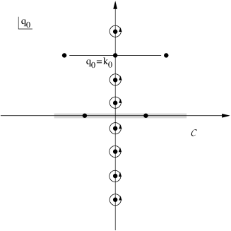
Figure 1: The contour ${\cal C}$ in Eq. (23) encloses the poles of $\tanh[q_{0}/(2T)]$ on the imaginary $q_{0}$ axis. The additional poles and the cut at $q_{0}=k_{0}$ arise from the gluon propagator, while the two poles on the real axis are due to the quasiquarks, cf. Eq. (20). The yet undetermined non-analyticities of the gap function on the real $q_{0}-$axis are indicated by the shaded area.

In order to introduce the spectral densities of the gap function and of the magnetic and longitudinal gluon propagators the contour ${\cal C}$ is deformed corresponding to Fig. 2.

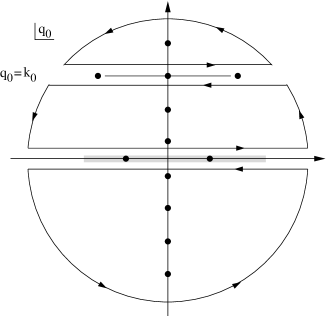
Figure 2: Deforming the contour ${\cal C}$ to introduce the spectral densities of $\Delta^{\ell,t}$ and $\phi$, cf. Eq. (24).

The contour integral can now be decomposed into three parts

$${\mathcal{M}}^{\ell,t}(k_{0},\mathbf{p},\mathbf{q})=I_{\infty}^{\ell,t}+I_{0}^{\ell,t}+I_{k_{0}}^{\ell,t}\;.$$ (24)

The first part, $I_{\infty}$, is the integral along a circle of asymptotically large radius. It can be estimated after parameterizing $dq_{0}=i|q_{0}|e^{i\theta}d\theta$ and considering the limit $|q_{0}|\rightarrow\infty$. To this end we write without loss of generality, cf. Appendix A,

$$\phi(K)\equiv\tilde{\phi}(K)+{\hat{\phi}}(\mathbf{k})\;,$$ (25)

so that the energy dependence of $\phi(K)$ is contained in $\tilde{\phi}(K)$. For asymptotically large energies, $|k_{0}|\rightarrow\infty$, we require that $\tilde{\phi}(K)\rightarrow 0$ and $\phi(K)\rightarrow{\hat{\phi}}(\mathbf{k})$, where ${\hat{\phi}}(\mathbf{k})$ is a real function of $\mathbf{k}$ only. Furthermore, we have $\Delta^{\ell}(Q-K)\rightarrow|\mathbf{q}-\mathbf{k}|^{-2}$ and $\Delta^{t}(Q-K)\rightarrow-q_{0}^{-2}$, cf. Eq. (107). It follows that the longitudinal contribution $I_{\infty}^{\ell}\sim q_{0}^{-1}$ and the transversal $I_{\infty}^{t}\sim q_{0}^{-3}$, and hence that in total $I_{\infty}^{\ell,t}\rightarrow 0$. The integral $I_{0}^{\ell,t}$ runs around the axis of real $q_{0}$,

$$I_{0}^{\ell,t}=\int\limits_{-\infty}^{\infty}\frac{dq_{0}}{2\pi i}\,\frac{1}{2}\tanh\left(\frac{q_{0}}{2T}\right)\Delta^{\ell,t}(Q-K)\left[\tilde{\Delta}(q_{0}+i\eta,\mathbf{q})\phi(q_{0}+i\eta,\mathbf{q})-\tilde{\Delta}(q_{0}-i\eta,\mathbf{q})\phi(q_{0}-i\eta,\mathbf{q})\right]\;.$$ (26)

Applying the Dirac identity and using Eq. (18) and $\phi(\omega+i\eta)+\phi(\omega-i\eta)=2{\rm Re}\,\phi(\omega)$ one obtains

$$I_{0}^{\ell,t} = \frac{1}{2{\tilde{\epsilon}_{\mathbf{q}}}}\sum\limits_{\sigma=\pm}\sigma{\mathcal{P}}_{\sigma{\tilde{\epsilon}_{\mathbf{q}}}}\int\limits_{-\infty}^{\infty}dq_{0}\frac{1}{2}\tanh\left(\frac{q_{0}}{2T}\right)\Delta^{\ell,t}(q_{0}-k_{0},\mathbf{p})Z^{2}(q_{0})\frac{\rho_{\phi}(q_{0},\mathbf{q})}{q_{0}-\sigma{\tilde{\epsilon}_{\mathbf{q}}}}$$ (27)

$$-\frac{1}{2{\tilde{\epsilon}_{\mathbf{q}}}}\frac{1}{2}\tanh\left(\frac{{\tilde{\epsilon}_{\mathbf{q}}}}{2T}\right)Z^{2}(\tilde{\epsilon}_{\mathbf{q}})\,{\rm Re}\,\phi({\tilde{\epsilon}_{\mathbf{q}}},\mathbf{q})\sum\limits_{\sigma=\pm}\Delta^{\ell,t}(\sigma{\tilde{\epsilon}_{\mathbf{q}}}-k_{0},\mathbf{p})\;,$$

where ${\mathcal{P}}_{x}$ denotes the principal value with respect to the pole at $x$. The first term arises from the non-analyticities of the gap function, cf. Eq. (18), and the second from the poles of the quark propagator at $q_{0}=\pm{\tilde{\epsilon}_{\mathbf{q}}}$, cf. Eq. (22).

The last integral $I_{k_{0}}^{\ell,t}$ circumvents the non-analyticities of the gluon propagator as well as the pole of $\tanh$. One finds

$$I_{k_{0}} = \frac{1}{2{\tilde{\epsilon}_{\mathbf{q}}}}\sum\limits_{\sigma=\pm}\sigma{\mathcal{P}}_{0}\int\limits_{-\infty}^{\infty}dq_{0}\frac{1}{2}\coth\left(\frac{q_{0}}{2T}\right)\phi(q_{0}+k_{0},\mathbf{q})\,Z^{2}(q_{0}+k_{0})\,\frac{\rho^{\ell,t}(q_{0},\mathbf{p})}{q_{0}-\sigma{\tilde{\epsilon}_{\mathbf{q}}}+k_{0}}$$ (28)

$$-T\,\Delta^{\ell,t}(0,\mathbf{p})\,\tilde{\Delta}(k_{0},\mathbf{q})\,\phi(k_{0},\mathbf{q})\;.$$

The first term is due to the non-analyticities of the longitudinal and magnetic gluon propagators, $\Delta^{\ell,t}$. The second arises from the pole of $\coth(q_{0}/2T)$ at $q_{0}=0$ and corresponds to the large occupation number density of gluons in the classical limit, $q_{0}\ll T$. This contribution has been shown to be beyond subleading order rdpdhr and will therefore be discarded in the following.

After analytical continuation, $k_{0}\rightarrow\omega+i\eta$, the Dirac identity is employed in order to split the complex gap equation (21) into its real and imaginary part. For its imaginary part one finds using Eqs. (27,28) and using the fact that Re$\,\phi(q_{0})$ and $Z^{2}(q_{0})$ are even functions

$${\rm Im\mathcal{M}}^{\ell,t}(\omega+i\eta,\mathbf{p},\mathbf{q}) = -\frac{\pi}{4{\tilde{\epsilon}_{\mathbf{q}}}}{\rm Re}\,\phi({\tilde{\epsilon}_{\mathbf{q}}},\mathbf{q})\,Z^{2}(\tilde{\epsilon}_{\mathbf{q}})\sum\limits_{\sigma=\pm}\sigma\rho^{\ell,t}({\omega-\sigma\tilde{\epsilon}_{\mathbf{q}}},\mathbf{p})\left[\tanh\left(\frac{\sigma{\tilde{\epsilon}_{\mathbf{q}}}}{2T}\right)+\coth\left(\frac{{\omega-\sigma\tilde{\epsilon}_{\mathbf{q}}}}{2T}\right)\right]$$ (29)

$$+\frac{\pi}{4{\tilde{\epsilon}_{\mathbf{q}}}}\sum\limits_{\sigma=\pm}\sigma{\mathcal{P}}\int\limits_{-\infty}^{\infty}dq_{0}\frac{\rho^{\ell,t}(\omega-q_{0},\mathbf{p})\rho_{\phi}(q_{0},\mathbf{q})}{q_{0}-\sigma{\tilde{\epsilon}_{\mathbf{q}}}}Z^{2}(q_{0})\left[\tanh\left(\frac{q_{0}}{2T}\right)+\coth\left(\frac{\omega-q_{0}}{2T}\right)\right]$$

$$\equiv {\rm Im\mathcal{M}}^{\ell,t}_{\cal A}(\omega+i\eta,\mathbf{p},\mathbf{q})+{\rm Im\mathcal{M}}^{\ell,t}_{\cal B}(\omega+i\eta,\mathbf{p},\mathbf{q})\,.$$

The first term on the r.h.s of Eq. (29), ${\rm Im\mathcal{M}}^{\ell,t}_{\cal A}$, contains all contributions to $\phi(K)$ that have already been considered in previous solutions to subleading order. Here the gap function is always on the quasiparticle mass-shell. The second term, ${\rm Im\mathcal{M}}^{\ell,t}_{\cal B}$, is due to the non-analyticities of $\phi(K)$. It has been neglected in all previous treatments due to the approximation

$$\rho_{\Xi}(\omega,\mathbf{q})\simeq-{\rm sign}(\omega)\,{\rm Re}\,\phi(\tilde{\epsilon}_{\mathbf{q}}+i\eta,\mathbf{q})\,Z^{2}(\tilde{\epsilon}_{\mathbf{q}})\,\delta\!\left(\omega^{2}-\tilde{\epsilon}_{\mathbf{q}}^{2}\right)\;,$$ (30)

cf. Eq. (41) in Ref. rdpdhr . By doing so, one always forces the gap function on the r.h.s. of the gap equation on the quasiparticle mass-shell. The gap equation takes then the standard form, cf. Eq. (19) of Ref. qwdhr . The occurrence of the external energy $\tilde{\epsilon}_{k}$ on the r.h.s. due to the energy-dependent gluon propagators indicates that the solution still possesses some energy dependence although not provided by the Ansatz.

In the limit of small temperatures, $T\rightarrow 0$, the hyperbolic functions in Eq. (29) simplify, yielding for $\omega>0$

$${\rm Im\mathcal{M}}^{\ell,t}_{T=0}(\omega+i\eta,\mathbf{p},\mathbf{q}) = \frac{\pi}{2{\tilde{\epsilon}_{\mathbf{q}}}}\left[\frac{}{}\!\!-Z^{2}(\tilde{\epsilon}_{\mathbf{q}})\,{\rm Re}\,\phi({\tilde{\epsilon}_{\mathbf{q}}},\mathbf{q})\,\rho^{\ell,t}(\omega-{\tilde{\epsilon}_{\mathbf{q}}},\mathbf{p})\,\theta(\omega-{\tilde{\epsilon}_{\mathbf{q}}})\right.$$ (31)

$$\left.+\sum\limits_{\sigma=\pm}\sigma\,{\mathcal{P}}\int\limits_{0}^{\omega}dq_{0}\;\frac{\rho^{\ell,t}(\omega-q_{0},\mathbf{p})\rho_{\phi}(q_{0},\mathbf{q})}{q_{0}-\sigma{\tilde{\epsilon}_{\mathbf{q}}}}\,Z^{2}(q_{0})\right]$$

$$\equiv {\rm Im\mathcal{M}}^{\ell,t}_{{\cal A},T=0}(\omega+i\eta,\mathbf{p},\mathbf{q})+{\rm Im\mathcal{M}}^{\ell,t}_{{\cal B},T=0}(\omega+i\eta,\mathbf{p},\mathbf{q})\;.$$ (32)

Inserting the Matsubara sums ${\rm Im\mathcal{M}}^{\ell,t}_{\cal A,B}$ back into Eq. (21),

$${\rm Im}\,\phi(\omega+i\eta,\mathbf{k}) = \frac{g^{2}}{3}\int\frac{d^{3}q}{(2\pi)^{3}}\sum\limits_{r=\ell,t}{\rm Tr}_{s}^{r}(k,p,q)\,\left[{\rm Im\mathcal{M}}^{r}_{\cal A}(\omega+i\eta,\mathbf{p},\mathbf{q})+{\rm Im\mathcal{M}}^{r}_{\cal B}(\omega+i\eta,\mathbf{p},\mathbf{q})\right]$$ (33)

$$\equiv {\cal A}(\omega+i\eta,\mathbf{k})+{\cal B}(\omega+i\eta,\mathbf{k})\;,$$ (34)

we have finally derived the gap equation for Im$\,\phi(\omega+i\eta,\mathbf{k})$. The traces over Dirac space are given by

$${\rm Tr}_{s}^{\ell}(k,p,q) = \frac{(k+q)^{2}-p^{2}}{2\,k\,q}\;,$$ (35a)

$${\rm Tr}_{s}^{t}(k,p,q) = -2-\frac{p^{2}}{2\,k\,q}+\frac{(k^{2}-q^{2})^{2}}{2\,k\,q\,p^{2}}\;.$$ (35b)

We found that the imaginary part of the gap function can be split into a term ${\cal A}(\omega+i\eta,\mathbf{k})$ which contains all contributions of the real part of the gap function on the quasiquark mass-shell, and a term ${\cal B}(\omega+i\eta,\mathbf{k})$ which contains all new contributions with the imaginary part of the gap function off the quasiparticle mass-shell, cf. Eq. (34). In the following it will be checked whether the known solution for Re$\,\phi(\tilde{\epsilon}_{\mathbf{k}},\mathbf{k})$, which neglects the contributions contained in $\cal B$, is self-consistent to subleading order. To this end, we can use the leading order solution for Re$\,\phi(\tilde{\epsilon}_{\mathbf{k}},\mathbf{k})$, which is given by DHRreview

$$\phi(y)\equiv\phi\,\sin\left(\frac{\pi\,y}{2}\right)\,\,,$$ (36)

where $\phi$ denotes the value of the gap function on the Fermi surface to leading logarithmic order in $g$ son

$$\phi\sim\mu\exp\left(-\frac{\pi}{2\,\bar{g}}\right)\;.$$ (37)

The variable $0\leq y\leq 1$ defines the distance from the Fermi surface through the mixed scale

$$\Lambda_{y}\equiv\phi^{y}M^{1-y}\;,$$ (38)

where $M\sim g\mu$ is defined in Eq. (14). A given value of $y$ corresponds to momenta $\mathbf{k}$ with $|k-\mu|\sim\Lambda_{y}$. Note that $\Lambda_{1}=\phi$ and $\Lambda_{0}=M$. Furthermore, we have $\Lambda_{\bar{g}}\sim e^{-\pi/2}\,M$, which is smaller but still of the order of $M$. Correspondingly, we refer to quarks with momenta $|k-\mu|\sim\Lambda_{1\leq y<\bar{g}}$ as exponentially close to the Fermi surface and to quarks with $|k-\mu|\sim\Lambda_{\bar{g}\geq y\geq 0}$ as farther away from the Fermi surface. Inserting $\phi(y)$ into ${\cal A}(\omega+i\eta,\mathbf{k})$ one can estimate ${\cal A}(\omega+i\eta,\mathbf{k})$ for different energy and momentum regimes. This is done in Sec. III.2. In the second iteration the part ${\cal B}(\omega+i\eta,\mathbf{k})$ is estimated by inserting $\rho_{\phi}\simeq{\cal A}/\pi$ into the expression for ${\cal B}(\omega+i\eta,\mathbf{k})$, which is done in Sec. III.3. In Sec. III.4 these estimates are used to write

$${\rm Re}\,\tilde{\phi}(\epsilon_{\mathbf{k}},\mathbf{k})=\frac{1}{\pi}\mathcal{P}\left[\;\int\limits_{0}^{\Lambda_{1}}+\int\limits_{\Lambda_{1}}^{\Lambda_{\bar{g}}}+\int\limits_{\Lambda_{\bar{g}}}^{\Lambda_{0}}+\cdots\right]d\omega\,\sum\limits_{\sigma=\pm}\frac{{\cal A}(\omega+i\eta,\mathbf{k})+{\cal B}(\omega+i\eta,\mathbf{k})}{\omega-\sigma\epsilon_{\mathbf{k}}}\;,$$ (39)

cf. Eq. (102a), where the integral over $\omega$ has been split according to the different energy regimes of the estimates for $\cal A$ and $\cal B$, cf. Table 1. Then, according to the discussion after Eq. (22), terms of order $g^{n}\phi$ contribute to the (sub)ⁿ-leading order to ${\rm Re}\,\tilde{\phi}(\epsilon_{\mathbf{k}},\mathbf{k})$. The main results of this analysis are summarized in Table 1 for momenta close to the Fermi surface, $|k-\mu|\ll M$.

 $\omega\lesssim\Lambda_{1}$   $\omega\sim\Lambda_{1>y>\bar{g}}$   $\omega\sim\Lambda_{\bar{g}>y>0}$   $\omega\sim m_{g}+\Lambda_{1>y>0}$   $M\lesssim\omega\lesssim 2\mu$  dominant gluons $t$-cut $t$-cut $t,\ell$-cut $\ell$-pole $t$-pole   ${\cal A}$   $g^{2}\phi$   $g\,\phi\,\cos\left(\frac{\pi\,y}{2}\right)$ $g\,\phi$   $g\,\phi\left(\frac{M}{\phi}\right)^{y}$ $g\,\phi$   ${\cal B}$   $g^{2}{\cal A}$  $g^{2}{\cal A}$ $g{\cal A}$   $g^{2}{\cal A}$ $g{\cal A}$   ${\cal H}\,[{\cal A}]$   $g^{2}\phi$  $\phi$ $g\,\phi$   $\phi$ $g\,\phi$   ${\cal H}\,[{\cal B}]$   $g^{4}\phi$  $g^{2}\phi$ $g^{2}\phi$   $g^{2}\phi$ $g^{2}\phi$

Table 1: Estimates for the terms ${\cal A}$ and ${\cal B}$, cf. Eq. (34), and for ${\cal H}\,[{\cal A}]$ and ${\cal H}\,[{\cal B}]$, cf. Eq. (39), for different energy scales and $|k-\mu|\ll M$. The gluon sectors dominating the respective energies are indicated.

The columns correspond to the various energy regimes of these estimates. In the first line the dominant gluon sectors are given. The cut of the transversal gluons gives the dominant contribution to ${\cal A}$ and ${\cal B}$ for energies smaller than the scale $M$. At the scale $M$, the longitudinal and the transversal cut contribute with the same magnitude. At that energy scale also the poles of the gluons start to contribute as soon as $\omega>m_{g}$. At energies just above $m_{g}$ the longitudinal pole dominates over the magnetic pole, whereas for larger energies up to $2\mu$ the transversal pole gives the leading contribution. The respective orders of magnitude of ${\cal A}$ and ${\cal B}$, estimated at the various energy scales, are given in the subsequent rows. It is found that either ${\cal B}\sim g{\cal A}$ or ${\cal B}\sim g^{2}{\cal A}$ and therefore ${\cal B\ll\cal A}$. Finally, the orders of magnitudes of the contributions to the Hilbert transforms ${\cal H}\,[{\cal A}]$ and ${\cal H}\,[{\cal B}]$, obtained by integrating over the respective energy scales, cf. Eq. (39), are listed. When calculating the Hilbert transform ${\cal H}\,[{\cal A}]$ up to energies $\omega\sim\Lambda_{\bar{g}}$, the transversal cut gives a contribution of order $\phi$, which is of leading order. Since ${\cal B}\sim g^{2}{\cal A}$ for these energies, ${\cal H}\,[{\cal B}]\sim g^{2}\phi$, i.e., the contributions from $\cal B$ are beyond subleading order. Integrating over larger energies $\omega\sim M$, it turns out that ${\cal H}\,[{\cal A}]\sim g\,\phi$, which gives a subleading-order contribution. Since ${\cal B}\sim g{\cal A}$ in this energy regime, the corresponding contribution from ${\cal H}\,[{\cal B}]$ is again beyond subleading order. For the contributions from the poles one finds that, in the region $\omega=m_{g}+\Lambda_{1>y>0}$, a contribution of order $\phi$ is generated by ${\cal H}\,[{\cal A}]$ (which combines with $\hat{\phi}(\mathbf{k})$ to give a contribution of order $g\,\phi$ in total, i.e., of subleading order). Since in this energy regime ${\cal B}\sim g^{2}{\cal A}$, the corresponding contribution ${\cal H}\,[{\cal B}]$ is again only of order $g^{2}\phi$, i.e., beyond subleading order. Integrating over large energies up to $2\mu$, ${\cal H}\,[{\cal A}]$ gives a contribution of order $g\,\phi$, which is of subleading order. Since in this regime ${\cal B}\sim g{\cal A}$, it follows that ${\cal H}\,[{\cal B}]$ is beyond subleading order.

In Sec. III.5 it is shown that also ${\hat{\phi}}(\mathbf{k})\sim\phi$ and that the imaginary part of the gap function again contributes to ${\hat{\phi}}(\mathbf{k})$ only at $g^{2}\phi$, i.e., beyond subleading order. This finally proves that the imaginary part of the gap function enters the real part only beyond subleading order. Hence, to subleading accuracy, the real part of the gap equation can be solved self-consistently neglecting the imaginary part of the gap function for quark momenta exponentially close to the Fermi surface. On the other hand, the real part of the gap function enters the imaginary part of the gap function always to leading order. For energies, for which ${\cal B}\sim g^{2}{\cal A}$, the imaginary part of the gap function can be calculated to subleading order from the real part alone. In particular, this is the case for the regime of small energies. Furthermore, since for these energies only the cut of magnetic gluons contributes, Im$\,\phi$ can be calculated to subleading order without much effort, which is done in Sec. III.7. In Sec. III.6, we reproduce the known gap equation for Re$\,\phi(\tilde{\epsilon}_{\mathbf{k}},\mathbf{k})$ by Hilbert transforming ${\cal A}(\omega+i\eta,\mathbf{k})$, cf. Eq. (102a), and adding the energy independent gap function $\hat{\phi}(\mathbf{k})$, cf. Eq. (25).

III.2 Estimating ${\cal A}$

For the purpose of estimating the various terms contributing to $\cal A$, cf.  Eqs. (31-34), one may restrict oneself to the leading contribution of the Dirac traces in Eq. (21), which is of order one. The integral over the absolute magnitude of the quark momentum is $\int dq\,q^{2}$, while the angular integration is $\int d\cos\theta\equiv\int dp\,p/(kq)$. Furthermore, we estimate $Z^{2}(\tilde{\epsilon}_{\mathbf{q}})\sim 1$. The contribution to $\cal A$ from ${\cal M}^{\ell,t}_{{\cal A},T=0}$ in Eq. (31), which arises from the cut of the soft gluon propagator, is

$${\cal A}^{\ell,t}_{\rm cut}(\omega,\mathbf{k}) \sim g^{2}\int\limits_{0}^{\delta}\frac{d\xi}{\epsilon_{\mathbf{q}}}\,{\rm Re}\,\phi(\epsilon_{\mathbf{q}},\mathbf{q})\int\limits_{\lambda}^{\Lambda_{\rm gl}}dp\,p\,\rho^{\ell,t}_{\rm cut}(\omega^{*},\mathbf{p})\;,$$ (40)

where $\omega^{*}\equiv\omega-\epsilon_{\mathbf{q}}$ and $0<\omega^{*}<\omega$. Furthermore, $\delta\equiv{{\rm min}(\omega,\Lambda_{\rm q})}$ and $\lambda\equiv{\max}(|\xi-\zeta|,\omega^{*})$ with $\zeta\equiv k-\mu$ and $\xi\equiv q-\mu$. In the effective theory, both $|\zeta|$ and $|\xi|$ are bounded by $\Lambda_{\rm q}\sim g\mu$. Due to the condition $\lambda<p<\Lambda_{\rm gl}$ it follows that ${\cal A}^{\ell,t}_{\rm cut}=0$ for $\omega>\Lambda_{\rm gl}+\Lambda_{\rm q}\simeq\mu$. For the purpose of power counting it is sufficient to employ the following approximative forms for $\rho^{\ell,t}_{\rm cut}$, cf. Eq. (110b,110d),

$$\rho_{\rm cut}^{t}(\omega^{*},{\bf p}) \simeq \frac{M^{2}}{\pi}\,\frac{\omega^{*}\,p}{p^{6}+(M^{2}\,\omega^{*})^{2}}\;,$$ (41a)

$$\rho^{\ell}_{\rm cut}(\omega^{*},{\bf p}) \simeq \frac{2M^{2}}{\pi}\,\frac{\omega^{*}}{p}\,\frac{1}{(p^{2}+3\,m_{g}^{2})^{2}}\;.$$ (41b)

These approximations reproduce the correct behavior for $\omega^{*}\ll p\ll m_{g}$, while for $\omega^{*}<p<\Lambda_{\rm gl}$ they give at least the right order of magnitude. With that the integration over $p$ can be performed analytically. For energies $\omega<\Lambda_{\rm gl}$ one finds for the transverse part

$${\cal A}^{t}_{\rm cut}(\omega,\mathbf{k}) \sim g^{2}\int\limits_{0}^{\delta}\frac{d\xi}{\epsilon_{\mathbf{q}}}\,{\rm Re}\,\phi(\epsilon_{\mathbf{q}},\mathbf{q})\left[\arctan\left(\frac{\Lambda_{\rm gl}^{3}}{M^{2}\omega^{*}}\right)-\arctan\left(\frac{\lambda^{3}}{M^{2}\omega^{*}}\right)\right]\;.$$ (42)

For all $\zeta\leq\Lambda_{\rm q}$ and $\omega\leq\Lambda_{\rm gl}$ one has $\Lambda_{\rm gl}^{3}/M^{2}\omega^{*}\gg 1$ and the first arctangent in the squared brackets may be set equal to $\pi/2$. In the case that $\omega\gg M$ one has $\lambda^{3}/M^{2}\omega^{*}\gg 1$ and the two arctangents cancel. If $\omega\sim M$, on the other hand, the arctangents combine to a number of order $1$. Finally, in the case that $\omega\sim\Lambda_{y}$ with $0\leq y\leq 1$, one has always $0\leq\xi\leq\Lambda_{y}$ due to the theta-function in Eq. (31). Moreover, it turns out that the arctangents cancel if $\zeta>\Lambda_{y/3}$, since then $\lambda^{3}/(M^{2}\omega^{*})\simeq\zeta^{3}/[M^{2}(\omega-\xi)]\gg 1$ for all $\xi<\omega$.

In the case that $\omega\sim\phi$, the integral over $\xi$ does not yield the BCS logarithm, cf. Appendix C, and we find

$${\cal A}^{t}_{\rm cut}(\phi,\mathbf{k}) \sim g^{2}\phi\;.$$ (43)

For larger energies $\omega\sim\Lambda_{y}$ with $0\leq y<1$ one substitutes $\xi(y^{\prime})\equiv\Lambda_{y^{\prime}}$, $d\xi/\xi=\ln(\phi/M)\,dy^{\prime}$ and obtains with Eq. (36)

$${\cal A}^{t}_{\rm cut}(\omega,\mathbf{k}) \sim g^{2}\,\ln\left(\frac{\phi}{M}\right)\phi\int\limits_{1}^{y}dy\,\sin\left(\frac{\pi\,y}{2}\right)\sim g\,\phi\,\cos\left(\frac{\pi\,y}{2}\right)\;.$$ (44)

Here, the integration over $0\leq\xi\leq\Lambda_{1}$ has been neglected, since it gives at most a contribution of order $g^{2}\phi$, cf. Eq. (43).

In the longitudinal sector one finds for the integral over the gluon momentum $p$

$${\cal I}(\lambda) \equiv M^{2}\int\limits_{\lambda}^{\Lambda_{\rm gl}}\frac{dp}{(p^{2}+X^{2})^{2}}\sim\frac{1}{X}\left[\arctan\left(\frac{\Lambda_{\rm gl}}{X}\right)-\arctan\left(\frac{\lambda}{X}\right)\right]-\frac{1}{\Lambda_{\rm gl}}\frac{\lambda^{2}-\lambda\Lambda_{\rm gl}+X^{2}}{\lambda^{2}+X^{2}}$$ (47)

$$\sim \left\{\begin{array}[]{c}\frac{1}{X}~{}~{}~{}~{}~{}~{},~{}{\rm for}~{}\lambda\leq X\\ \frac{\Lambda_{\rm gl}-\lambda}{\Lambda_{\rm gl}\lambda}~{}~{},~{}{\rm for}~{}\lambda\gg X\end{array}\right.\;,$$

where $X^{2}\equiv 3m_{g}^{2}$. Since $\zeta\leq\Lambda_{\rm q}\sim X$, solely the magnitude of $\omega$ decides whether $\lambda\leq X$ or $\lambda\gg X$ is realized. It follows that, in contrast to the transversal case, the order of magnitude of ${\cal A}^{\ell}_{\rm cut}$ is independent of $\zeta$. Energies $\omega\sim\Lambda_{0\leq y\leq 1}$ correspond to $\lambda\leq X$. For the special case $\omega\sim\Lambda_{1}$ one finds

$${\cal A}^{\ell}_{\rm cut}(\omega,\mathbf{k}) \sim g^{2}\int\limits_{0}^{\Lambda_{1}}\frac{d\xi}{\epsilon_{\mathbf{q}}}\,{\rm Re}\,\phi(\epsilon_{\mathbf{q}},\mathbf{q})\,\,\frac{\omega^{*}}{M}\sim g^{2}\,\phi\,\frac{\phi}{M}\;.$$ (48)

For $\omega\sim\Lambda_{0\leq y<1}$ one obtains

$${\cal A}^{\ell}_{\rm cut}(\omega,\mathbf{k}) \sim g\,\phi\int\limits_{1}^{y}dy^{\prime}\,\sin\left(\frac{\pi\,y^{\prime}}{2}\right)\,\frac{\omega^{*}}{M}\sim g\,\phi\int\limits_{1}^{y}dy^{\prime}\,\sin\left(\frac{\pi\,y^{\prime}}{2}\right)\,\left[\left(\frac{\phi}{M}\right)^{y}-\left(\frac{\phi}{M}\right)^{y^{\prime}}\right]$$ (49)

$$\sim g\,\phi\,\cos\left(\frac{\pi\,y}{2}\right)\,\left(\frac{\phi}{M}\right)^{y}\;.$$

Hence, for $y>0$ the term ${\cal A}^{\ell}_{\rm cut}$ is suppressed by a factor $(\phi/M)^{y}$ as compared to ${\cal A}^{t}_{\rm cut}$ whereas for $y=0$ the longitudinal and the transversal cut contribute at the same order, ${\cal A}^{\ell}_{\rm cut}\sim{\cal A}^{t}_{\rm cut}\sim g\,\phi$. For much larger energies, $M\ll\omega<\mu$, we have $\lambda=\omega^{*}\simeq\omega\gg X$ (note that $\zeta$ is bounded by $\Lambda_{\rm q}$). It follows with $\delta=\Lambda_{\rm q}\sim\Lambda_{0}$

$${\cal A}^{\ell}_{\rm cut}(\omega,\mathbf{k}) \sim g\,\phi\int\limits_{1}^{0}dy\,\sin\left(\frac{\pi\,y}{2}\right)\,\left(1-\frac{\omega}{\Lambda_{\rm gl}}\right)\sim g\,\phi\left(1-\frac{\omega}{\mu}\right)\;.$$ (50)

Hence, ${\cal A}^{\ell}_{\rm cut}\gg{\cal A}^{t}_{\rm cut}$ in this large-energy regime. The results for ${\cal A}^{\ell,t}_{\rm cut}$ are summarized in Tables 2 and 3.

$\omega\sim\phi$ $\omega\sim\Lambda_{1>y>0}$  $\omega\sim M$  $M\ll\omega<\mu$   ${\cal A}_{\rm cut}^{t}$ $g^{2}\phi$ $g\,\phi\,\cos\left(\frac{\pi\,y}{2}\right)$ $g\,\phi$ 0 ${\cal A}_{\rm cut}^{\ell}$   $g^{2}\phi\,\frac{\phi}{M}$  $g\,\phi\left(\frac{\phi}{M}\right)^{y}\cos\left(\frac{\pi\,y}{2}\right)$ $g\,\phi$  $g\,\phi\left(1-\frac{\omega}{\mu}\right)$

Table 2: Estimates for ${\cal A}_{\rm cut}^{\ell,t}$ at different energy scales and $\zeta\ll M$.

$\omega\sim\phi$ $\omega\sim\Lambda_{1>y>0}$  $\omega\sim M$  $M\ll\omega<\mu$   ${\cal A}_{\rm cut}^{t}$ 0 0 $g\,\phi$ 0 ${\cal A}_{\rm cut}^{\ell}$   $g^{2}\phi\,\frac{\phi}{M}$  $g\,\phi\left(\frac{\phi}{M}\right)^{y}\cos\left(\frac{\pi\,y}{2}\right)$ $g\,\phi$ $~{}g\,\phi\left(1-\frac{\omega}{\mu}\right)$

Table 3: Estimates for ${\cal A}_{\rm cut}^{\ell,t}$ at different energy scales and $\zeta\lesssim M$.

The contributions from the gluon poles to $\cal A$ read analogously to Eq. (40)

$${\cal A}^{\ell,t}_{\rm pole}(\omega,\mathbf{k}) \sim g^{2}\int\limits_{0}^{\delta}\frac{d\xi}{\epsilon_{\mathbf{q}}}\,{\rm Re}\,\phi(\epsilon_{\mathbf{q}},\mathbf{q})\int\limits_{|\xi-\zeta|}^{2\mu}dp\,p\,\rho^{\ell,t}_{\rm pole}(\omega^{*},\mathbf{p})\,\delta[\omega^{*}-\omega_{\ell,t}(\mathbf{p})]\;.$$ (51)

The boundary $p\leq 2\mu$ in the integral over $p$ is due to the constraint $\xi\leq\Lambda_{\rm q}$, cf. Fig. 3.

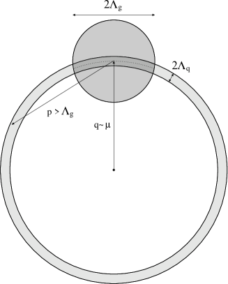
Figure 3: Hard gluon exchange with momentum $p>\Lambda_{\rm gl}\sim\mu$. The quark has to remain within a layer of width $2\Lambda_{\rm q}\sim g\mu$ around the Fermi surface. This effectively restricts the hard gluon momentum to $p<2\mu+2\Lambda_{\rm q}\lesssim 2\mu$.

Therefore, also $\omega_{\ell,t}<2\mu$. It follows that ${\cal A}^{\ell,t}_{\rm pole}=0$ for $\omega>2\mu$, since for these energies one has $\omega^{*}\simeq\omega>\omega_{\ell,t}$ always and the $\delta-$function in Eq. (51) vanishes. Hence, we can restrict the analysis of Eq.  (51) to $m_{g}<\omega<2\mu$.

For the transverse sector we approximate

$$\rho^{t}_{\rm pole}(\omega_{t}(\mathbf{p}),\mathbf{p})\simeq-\frac{1}{2\omega_{t}(\mathbf{p})}$$ (52)

and $\omega_{t}(\mathbf{p})\simeq\sqrt{p^{2}+m_{g}^{2}}$ for all momenta $p$ and obtain

$${\cal A}^{t}_{\rm pole}(\omega,\mathbf{k}) \sim g^{2}\int\limits_{0}^{\Lambda_{\rm q}}\frac{d\xi}{\epsilon_{\mathbf{q}}}\,{\rm Re}\,\phi(\epsilon_{\mathbf{q}},\mathbf{q})\!\!\!\!\int\limits_{\sqrt{m_{g}^{2}+|\zeta-\xi|^{2}}}^{2\mu}\!\!\!\!\!\!d\omega_{t}\,\delta(\omega^{*}-\omega_{t})\;.$$ (53)

The condition $\omega^{*}=\omega_{t}$ can be satisfied only if $\omega>\sqrt{m_{g}^{2}+\zeta^{2}}$. Furthermore, the condition $\omega^{*}=\omega_{t}$ sets an upper boundary to the integral over $\xi$ given by $\xi_{\rm max}\equiv{\rm min}\{\Lambda_{\rm q},(\omega^{2}-m_{g}^{2}-\zeta^{2})/2(\omega-\zeta)\}$. Hence, the BCS logarithm is generated for energies $\omega\sim\sqrt{m_{g}^{2}+\zeta^{2}}+\Lambda_{y}$ with $0\leq y<1$, since then $\xi_{\rm max}\sim\Lambda_{y}$. For such energies we have

$${\cal A}^{t}_{\rm pole}(\omega,\mathbf{k}) \sim g^{2}\int\limits_{0}^{\xi_{\rm max}}\frac{d\xi}{\epsilon_{\mathbf{q}}}\,{\rm Re}\,\phi(\epsilon_{\mathbf{q}},\mathbf{q})\sim g\,\phi\,\cos\left(\frac{\pi\,y}{2}\right)\;.$$ (54)

For larger energies up to $2\mu$ one has ${\cal A}^{t}_{\rm pole}(\omega,\mathbf{k})\sim g\,\phi$.

In the longitudinal gluon sector we approximate

$$\rho^{\ell}_{\rm pole}(\omega_{\ell}(\mathbf{p}),\mathbf{p})\simeq-\frac{\omega_{\ell}(\mathbf{p})}{2p^{2}}$$ (55)

for gluon momenta $p$ not much larger than $m_{g}$. Such values of $p$ are guaranteed if we consider energies of the form $\omega=\sqrt{m_{g}^{2}+\zeta^{2}}+\Lambda_{y_{1}}$ with $\bar{g}<y_{1}<1$. As in the transversal case we simplify $\omega_{\ell}(\mathbf{p})\simeq\sqrt{p^{2}+m_{g}^{2}}$ and find

$${\cal A}^{\ell}_{\rm pole}(\omega,\mathbf{k}) \sim g^{2}\int\limits_{0}^{\xi_{\rm max}}\frac{d\xi}{\epsilon_{\mathbf{q}}}\,{\rm Re}\,\phi(\epsilon_{\mathbf{q}},\mathbf{q})\!\!\!\!\int\limits_{\sqrt{m_{g}^{2}+|\xi-\zeta|^{2}}}^{2\mu}\!\!\!\!\!\!d\omega_{\ell}\,\frac{\omega_{\ell}^{2}}{\omega^{2}_{\ell}-m_{g}^{2}}\,\delta(\omega^{*}-\omega_{\ell})\;,$$ (56)

where $\xi_{\rm max}$ is defined as in the transversal case. For the considered energies one has $\xi_{\rm max}\sim\Lambda_{y_{1}}$. We find

$${\cal A}^{\ell}_{\rm pole}(\omega,\mathbf{k}) \sim g^{2}\int\limits_{0}^{\xi_{\rm max}}\frac{d\xi}{\epsilon_{\mathbf{q}}}\,{\rm Re}\,\phi(\epsilon_{\mathbf{q}},\mathbf{q})\frac{(\omega-\epsilon_{\mathbf{q}})^{2}}{(\omega-\epsilon_{\mathbf{q}})^{2}-m_{g}^{2}}$$ (57)

$$\sim g\,\phi\,\frac{\omega}{\omega-m_{g}}\,\cos\left(\frac{\pi\,y_{1}}{2}\right)\;,$$

where $\xi_{\rm max}\ll\omega$ and $\omega\gtrsim m_{g}$ was exploited in order to simplify the fraction under the integral, $\omega^{2}/(\omega^{2}-m_{g}^{2})\sim\omega/(\omega-m_{g})$. Furthermore, the BCS logarithm has cancelled one power of $g$. Hence, for $\zeta\sim m_{g}$ one has ${\cal A}^{\ell}_{\rm pole}\sim g\,\phi$. For quarks exponentially close to the Fermi surface with $\zeta\sim\Lambda_{y_{2}/2}$ and $y_{2}>2\,\bar{g}$, we find

$${\cal A}^{\ell}_{\rm pole}(\omega,\mathbf{k})\sim g\,\phi\,\left(\frac{M}{\phi}\right)^{y}\cos\left(\frac{\pi\,y_{1}}{2}\right)\;,$$ (58)

where $y\equiv{\rm min}\{y_{1},y_{2}\}$. For much larger energies, $\omega\gg m_{g}$, we have to consider gluon momenta $p\gg m_{g}$, for which the spectral density of longitudinal gluons is exponentially suppressed

$$\rho_{\rm pole}^{\ell}(\omega_{l}(\mathbf{p}),\mathbf{p})\sim\frac{\exp\left(-\frac{2p^{2}}{3m_{g}^{2}}\right)}{p}\;.$$ (59)

We find for $m_{g}\ll\omega<2\mu$ with $\omega_{l}(\mathbf{p})\simeq p$

$${\cal A}^{\ell}_{\rm pole}(\omega,\mathbf{k}) \sim g^{2}\int\limits_{0}^{\Lambda_{\rm q}}\frac{d\xi}{\epsilon_{\mathbf{q}}}\,{\rm Re}\,\phi(\epsilon_{\mathbf{q}},\mathbf{q})\!\!\!\!\int\limits_{\sqrt{m_{g}^{2}+|\xi-\zeta|^{2}}}^{2\mu}\!\!\!\!\!\!d\omega_{\ell}\,\exp\left(-\frac{2\omega_{\ell}^{2}}{3m_{g}^{2}}\right)\,\delta(\omega^{*}-\omega_{\ell})$$ (60)

$$\sim g^{2}\phi\int\limits_{\Lambda_{1}}^{\Lambda_{0}}\frac{d\xi}{\xi}\,\exp\left[-\frac{2(\omega-\xi)^{2}}{3m_{g}^{2}}\right]\sim g\,\phi\,\exp\left(-\frac{2\omega^{2}}{3m_{g}^{2}}\right)\;,$$

which is the continuation of Eq. (57) to large energies and for all $\zeta\leq\Lambda_{\rm q}$. The results for ${\cal A}^{\ell,t}_{\rm pole}$ are summarized in Table 4.

  $\omega<\sqrt{m_{g}^{2}+\zeta^{2}}~{}$   $\omega\sim\sqrt{m_{g}^{2}+\zeta^{2}}+\Lambda_{1<y_{1}<\bar{g}}$  $m_{g}\ll\omega<2\mu$   ${\cal A}_{\rm pole}^{t}$ 0 $g\,\phi$ $g\,\phi$ ${\cal A}_{\rm pole}^{\ell}$ 0 $g\,\phi\left(\frac{M}{\phi}\right)^{y}\cos\left(\frac{\pi\,y_{1}}{2}\right)$   $g\,\phi\,\exp\left(-\frac{2\omega^{2}}{3m_{g}^{2}}\right)$

Table 4: Estimates for ${\cal A}_{\rm pole}^{\ell,t}$ at different energy scales and for $\zeta\sim\Lambda_{y_{2}}$, where $0\leq y_{2}\leq 1$ and $y\equiv{\rm min}\{y_{1},y_{2}\}$.

In the following Sec. III.3 these results will be inserted into Eq. (31) for $\rho_{\phi}$ in order to estimate $\cal B$.

III.3 Estimating ${\cal B}$

The term ${\cal B}$ in Eq. (34) can be estimated using

$${\cal B}^{\ell,t}_{\rm cut}(\omega,\mathbf{k})\sim g^{2}\int\limits_{0}^{\Lambda_{\rm q}}\frac{d\xi}{\epsilon_{\mathbf{q}}}\int\limits_{0}^{\omega}dq_{0}\sum\limits_{\sigma=\pm}\frac{\sigma\,{\cal A}(q_{0},\mathbf{q})}{q_{0}-\sigma\epsilon_{\mathbf{q}}}\int\limits_{\lambda}^{\Lambda_{\rm gl}}dp\,p\,\rho^{\ell,t}_{\rm cut}(\omega^{\prime},\mathbf{p})\;,$$ (61)

for the Landau-damped gluon sector. We introduced $\omega^{\prime}\equiv\omega-q_{0}<\omega$ and $\lambda\equiv{\max}(|\xi-\zeta|,\omega^{\prime})$. Furthermore, we set $Z^{2}(\omega)\sim 1$. From the condition $\lambda<\Lambda_{\rm gl}$ in Eq. (61) and from ${\cal A}(q_{0},\mathbf{q})=0$ for $q_{0}>2\mu$ it follows that ${\cal B}^{\ell,t}_{\rm cut}(\omega,\mathbf{k})=0$ for $\omega>\Lambda_{\rm gl}+2\mu\sim 3\mu$. Inserting the approximative forms (41) for $\rho^{\ell,t}_{\rm cut}$ into Eq. (61) the integration over $p$ can be performed analogously to Eqs. (42,47). In the transverse case one finds

$${\cal B}^{t}_{\rm cut}(\omega,\mathbf{k})\sim g^{2}\int\limits_{0}^{\Lambda_{\rm q}}\frac{d\xi}{\epsilon_{\mathbf{q}}}\int\limits_{0}^{\omega}dq_{0}\sum\limits_{\sigma=\pm}\frac{\sigma\,{\cal A}(q_{0},\mathbf{q})}{q_{0}-\sigma\epsilon_{\mathbf{q}}}\left[\arctan\left(\frac{\Lambda_{\rm gl}^{3}}{M^{2}\omega^{\prime}}\right)-\arctan\left(\frac{\lambda^{3}}{M^{2}\omega^{\prime}}\right)\right]\;.$$ (62)

Analogously to Eq. (42), one first determines the domains of $\omega,\,\zeta$, and $\xi$, where the arctangents in the squared brackets do not cancel. Since $\omega^{\prime}<\omega<3\mu$ it is $\Lambda_{\rm gl}^{3}/M^{2}\omega^{\prime}\gg 1$ and the first arctangent in the squared brackets may be set equal to $\pi/2$. Furthermore, one finds that the argument of the second arctangent is not very large as long as the conditions $\omega-M\lesssim q_{0}$ and $|\xi-\zeta|^{3}\lesssim M^{2}(\omega-q_{0})$ are fulfilled. In order to satisfy the first condition, we restrict the integral over $q_{0}$ to the region ${\rm max}\{0,\omega-M\}<q_{0}<\omega$. The second condition becomes less restrictive if simplified to $|\xi-\zeta|^{3}\lesssim M^{2}\omega$. The resulting estimate for ${\cal B}^{t}_{\rm cut}$ will turn out to be small so that a more elaborate estimate is not necessary. For energies $\omega\sim\phi$ one may use Eq. (43) to estimate ${\cal A}\sim{\cal A}^{t}_{\rm cut}\sim g^{2}\phi$. For $\zeta\ll M$ one has

$${\cal B}^{t}_{\rm cut}(\phi,\mathbf{k})\sim g^{4}\phi\int\limits_{0}^{\Lambda_{1/3}}\frac{d\xi}{\epsilon_{\mathbf{q}}}\,\ln\left|\frac{\epsilon_{\mathbf{q}}-\phi}{\epsilon_{\mathbf{q}}+\phi}\right|\sim g^{4}\phi\;.$$ (63)

The logarithm under the integral prevents the generation of the BCS logarithm, cf. Appendix C. For $\zeta\lesssim M$ the integration over $\xi$ is restricted to the region $|\xi-\zeta|<\Lambda_{1/3}$. This yields the estimate ${\cal B}^{t}_{\rm cut}(\phi,\mathbf{k})\sim g^{4}\phi\,(\Lambda_{1/3}/M)\sim g^{4}\phi\,(\phi/M)^{1/3}$.

For $\omega\sim\Lambda_{y}$ with $0\leq y<1$ we conservatively estimate ${\cal A}\sim{\cal A}^{t}_{\rm cut}\sim g\,\phi$, cf. Eq. (44), and obtain similarly to Eq. (63)

$${\cal B}^{t}_{\rm cut}(\Lambda_{y},\mathbf{k})\sim g^{3}\phi\int\limits_{0}^{\Lambda_{y/3}}\frac{d\xi}{\epsilon_{\mathbf{q}}}\,\ln\left|\frac{\epsilon_{\mathbf{q}}-\Lambda_{y}}{\epsilon_{\mathbf{q}}+\Lambda_{y}}\right|\sim g^{3}\phi\;,$$ (64)

where we assumed $\zeta\ll M$. Again no BCS logarithm was generated due to the additional logarithm. For $\zeta\lesssim M$ the integration over $\xi$ is restricted to the region $|\xi-\zeta|<\Lambda_{y/3}$. If we conservatively estimate ${\cal A}\sim g\,\phi$ throughout this region, we obtain ${\cal B}^{t}_{\rm cut}(\phi,\mathbf{k})\sim g^{3}\phi\,(\phi/M)^{y/3}$.

For energies $\omega\sim M$ and larger, the condition $|\xi-\zeta|^{3}\lesssim M^{2}\omega$ is fulfilled for all $\xi<\Lambda_{\rm q}$. Considering $\omega\sim m_{g}+\Lambda_{y}$ with $0\leq y<1$ we find that the dominant contribution comes from ${\cal A}\sim{\cal A}^{\ell}_{\rm pole}$, cf. Eq. (58), when integrating over $m_{g}+\Lambda_{1}<q_{0}<m_{g}+\Lambda_{y}$

$${\cal B}^{t}_{\rm cut}(m_{g}+\Lambda_{y},\mathbf{k}) \sim g^{3}\phi\int\limits_{0}^{\Lambda_{\rm q}}\frac{d\xi}{\epsilon_{\mathbf{q}}}\int\limits_{m_{g}+\Lambda_{1}}^{m_{g}+\Lambda_{y}}dq_{0}\sum\limits_{\sigma=\pm}\frac{\sigma}{q_{0}-\sigma\epsilon_{\mathbf{q}}}\,\frac{q_{0}}{q_{0}-m_{g}}$$ (65)

$$\sim g^{2}\phi\int\limits_{0}^{\Lambda_{\rm q}}\frac{d\xi}{\epsilon_{\mathbf{q}}}\,\sum\limits_{\sigma=\pm}\frac{\sigma\,m_{g}}{\sigma\epsilon_{\mathbf{q}}-m_{g}}\int\limits_{1}^{y}dy^{\prime}\sim g^{2}\phi\int\limits_{0}^{\Lambda_{\rm q}}d\xi\,\frac{m_{g}}{\xi^{2}-m_{g}^{2}}$$

$$\sim g^{2}\,\phi\;.$$

The contributions from the other gluon sectors are estimated with ${\cal A}\sim g\,\phi$, cf. Eqs. (50,56),

$$g^{3}\phi\int\limits_{0}^{\Lambda_{\rm q}}\frac{d\xi}{\epsilon_{\mathbf{q}}}\int\limits_{\omega-M}^{\omega}dq_{0}\,\sum\limits_{\sigma=\pm}\frac{\sigma}{q_{0}-\sigma\epsilon_{\mathbf{q}}} \sim g^{3}\phi\int\limits_{0}^{\Lambda_{\rm q}}\frac{d\xi}{\epsilon_{\mathbf{q}}}\left(\ln\left|\frac{\omega-\epsilon_{q}}{\epsilon_{q}+\omega}\right|-\ln\left|\frac{\omega-M+\epsilon_{q}}{\omega-M-\epsilon_{q}}\right|\right)$$ (66)

$$\sim g^{3}\phi\left(\frac{M}{\omega}\right)^{2}\;,$$

where the logarithms again prevent the generation of the BCS logarithm. The factor $(M/\omega)^{2}$ arises from expanding the logarithms for $\omega\gg M$. Hence, for energies of the form $\omega\sim m_{g}+\Lambda_{y}$ with $0\leq y<1$ we have

$${\cal B}^{t}_{\rm cut}(\omega,\mathbf{k}) \sim g^{2}\phi\;,$$ (67)

while for larger energies ${\cal A}^{\ell}_{\rm pole}$ does not contribute anymore and ${\cal B}^{t}_{\rm cut}(\omega,\mathbf{k})\sim g^{3}\phi\,(M/\omega)^{2}$, cf.  Eq. (66).

For the cut of the longitudinal gluons one obtains

$${\cal B}^{\ell}_{\rm cut}(\omega,\mathbf{k}) \sim g^{2}\int\limits_{0}^{\Lambda_{\rm q}}\frac{d\xi}{\epsilon_{\mathbf{q}}}\int\limits_{0}^{\omega}dq_{0}\sum\limits_{\sigma=\pm}\frac{\sigma\,{\cal A}(q_{0},\mathbf{q})}{q_{0}-\sigma\epsilon_{\mathbf{q}}}\;\omega^{\prime}\;{\cal I}(\lambda)\;,$$ (68)

where ${\cal I}(\lambda)$ is defined in Eq. (47). Analogously to the analysis of ${\cal A}_{\rm cut}^{\ell}$ one finds for $\omega\sim\phi$

$${\cal B}^{\ell}_{\rm cut}(\phi,\mathbf{k}) \sim g^{4}\phi\int\limits_{0}^{\Lambda_{\rm q}}\frac{d\xi}{\epsilon_{\mathbf{q}}}\int\limits_{0}^{\phi}dq_{0}\sum\limits_{\sigma=\pm}\frac{\sigma}{q_{0}-\sigma\epsilon_{\mathbf{q}}}\,\frac{\phi}{M}\sim g^{4}\phi\,\frac{\phi}{M}\int\limits_{0}^{\Lambda_{\rm q}}\frac{d\xi}{\epsilon_{\mathbf{q}}}\,\ln\left|\frac{\epsilon_{\mathbf{q}}-\phi}{\epsilon_{\mathbf{q}}+\phi}\right|$$ (69)

$$\sim g^{4}\phi\,\frac{\phi}{M}\;,$$

and similarly for $\omega\sim\Lambda_{y}$ with $0\leq y<1$

$${\cal B}^{\ell}_{\rm cut}(\Lambda_{y},\mathbf{k})\sim g^{3}\phi\left(\frac{\phi}{M}\right)^{y}\;.$$ (70)

For $\omega\sim m_{g}+\Lambda_{y}$ with $0\leq y<1$ we can simplify $\omega^{\prime}\,{\cal I}(\lambda)\simeq 1$ and find as in the transversal case, cf. Eq. (65),

$${\cal B}^{\ell}_{\rm cut}(m_{g}+\Lambda_{y},\mathbf{k}) \sim g^{2}\phi\;.$$ (71)

In the limit of large energies, $M\ll\omega\sim\Lambda_{\rm gl}\sim\mu$, we estimate the integral over the range $\omega-\Lambda_{\rm gl}<q_{0}<\omega$ by substituting ${\cal A}\sim g\,\phi$ and obtain with $\omega^{\prime}\,{\cal I}(\lambda)\sim 1$

$${\cal B}^{\ell}_{\rm cut}(\omega,\mathbf{k}) \sim g^{3}\phi\int\limits_{0}^{\Lambda_{\rm q}}\frac{d\xi}{\epsilon_{\mathbf{q}}}\int\limits_{\omega-\Lambda_{\rm gl}}^{\omega}dq_{0}\sum\limits_{\sigma=\pm}\frac{\sigma}{q_{0}-\sigma\epsilon_{\mathbf{q}}}\sim g^{3}\phi\int\limits_{0}^{\Lambda_{\rm q}}d\xi\int\limits_{\omega-\Lambda_{\rm gl}}^{\omega}\frac{dq_{0}}{q_{0}^{2}}$$ (72)

$$\sim g^{3}\phi\,\frac{M\Lambda_{\rm gl}}{\omega^{2}}\sim g^{3}\phi\,\frac{M}{\omega}\;.$$

Hence, also ${\cal B}^{\ell}_{\rm cut}$ becomes small in the limit of large energies. The estimates for ${\cal B}^{\ell,t}_{\rm cut}$ are summarized in Tables 6 and 6.

  $\omega\sim\phi$   $\omega\sim\Lambda_{1>y>0}$  $\omega\sim m_{g}+\Lambda_{1>y>0}$  $m_{g}\ll\omega<3\mu$   ${\cal B}_{\rm cut}^{t}$ $g^{4}\phi$ $g^{3}\phi$ $g^{2}\phi$ $g^{3}\phi\left(\frac{M}{\omega}\right)^{2}$ ${\cal B}_{\rm cut}^{\ell}$  $g^{4}\phi\,\frac{\phi}{M}$   $g^{3}\phi\left(\frac{\phi}{M}\right)^{y}$ $g^{2}\phi$   $g^{3}\phi\,\frac{M}{\omega}$

Table 5: Estimates for ${\cal B}_{\rm cut}^{\ell,t}$ at different energy scales and $\zeta\ll M$.

  $\omega\sim\phi$   $\omega\sim\Lambda_{1>y>0}$  $\omega\sim m_{g}+\Lambda_{1>y>0}$  $m_{g}\ll\omega<3\mu$   ${\cal B}_{\rm cut}^{t}$ $~{}g^{4}\phi\,\left(\frac{\phi}{M}\right)^{1/3}~{}$ $~{}g^{3}\phi\,\left(\frac{\phi}{M}\right)^{y/3}$ $g^{2}\phi$ $g^{3}\phi\left(\frac{M}{\omega}\right)^{2}$ ${\cal B}_{\rm cut}^{\ell}$  $g^{4}\phi\,\frac{\phi}{M}$   $g^{3}\phi\left(\frac{\phi}{M}\right)^{y}$ $g^{2}\phi$   $g^{3}\phi\,\frac{M}{\omega}$

Table 6: Estimates for ${\cal B}_{\rm cut}^{\ell,t}$ at different energy scales and $\zeta\lesssim M$.

In the undamped gluon sector the term ${\cal M}^{\ell,t}_{{\cal B},T=0}$ in Eq. (31) gives the contribution

$${\cal B}^{\ell,t}_{\rm pole}(\omega,\mathbf{k})\sim g^{2}\int\limits_{0}^{\Lambda_{\rm q}}\frac{d\xi}{\epsilon_{\mathbf{q}}}\int\limits_{0}^{\omega}dq_{0}\sum\limits_{\sigma=\pm}\frac{\sigma\,\rho_{\phi}(q_{0},\mathbf{q})}{q_{0}-\sigma\epsilon_{\mathbf{q}}}\int\limits_{|\zeta-\xi|}^{2\mu}dp\,p\,\rho^{\ell,t}_{\rm pole}(\omega^{\prime},\mathbf{p})\,\delta[\omega^{\prime}-\omega_{\ell,t}(\mathbf{p})]\;.$$ (73)

Due to the restriction $p<2\mu$ it follows with similar arguments as for ${\cal B}^{\ell,t}_{\rm cut}$ that ${\cal B}^{\ell,t}_{\rm pole}(\omega,\mathbf{k})=0$ for $\omega>4\mu$. For the transversal sector we employ analogous approximations as for ${\cal A}^{t}_{\rm pole}$ and obtain

$${\cal B}^{t}_{\rm pole}(\omega,\mathbf{k}) \sim g^{2}\int\limits_{\Lambda_{1}}^{\Lambda_{0}}\frac{d\xi}{\xi}\int\limits_{0}^{\omega}dq_{0}\sum\limits_{\sigma=\pm}\frac{\sigma\,{\cal A}(q_{0},\mathbf{q})}{q_{0}-\sigma\epsilon_{\mathbf{q}}}\int\limits_{\sqrt{m_{g}^{2}+|\xi-\zeta|^{2}}}^{2\mu}\!\!\!d\omega_{t}\,\delta(\omega^{\prime}-\omega_{t})\;.$$ (74)

This contribution is non-zero only if $\omega>m_{g}$. First we consider energies $\omega\sim m_{g}+\Lambda_{2y_{1}}$ and $\zeta\sim\Lambda_{y_{2}}$, and analyze the two cases $y_{1}<y_{2}$ and $y_{1}>y_{2}$ separately. In the first case, the condition $\omega>\sqrt{m_{g}^{2}+|\xi-\zeta|^{2}}$ requires $0<\xi<\Lambda_{y_{1}}$ and consequently

$${\cal B}^{t}_{\rm pole}(\omega,\mathbf{k}) \sim g^{3}\phi\int\limits_{\Lambda_{1}}^{\Lambda_{y_{1}}}\frac{d\xi}{\xi}\,\,\ln\left|\frac{\omega-\sqrt{m_{g}^{2}+\xi^{2}}-\xi}{\omega-\sqrt{m_{g}^{2}+\xi^{2}}+\xi}\right|\sim g^{3}\phi\;,$$ (75)

where ${\cal A}\sim g\,\phi$ and the logarithm prevents the BCS logarithm. The second case, $y_{1}>y_{2}$, leads to the condition $\Lambda_{y_{2}}-\Lambda_{y_{1}}<\xi<\Lambda_{y_{2}}+\Lambda_{y_{1}}$ and we find

$${\cal B}^{t}_{\rm pole}(\omega,\mathbf{k}) \sim g^{3}\phi\int\limits_{\Lambda_{y_{2}}-\Lambda_{y_{1}}}^{\Lambda_{y_{2}}+\Lambda_{y_{1}}}\frac{d\xi}{\xi}\,\ \ln\left|\frac{m_{g}-\sqrt{m_{g}^{2}+\Lambda_{y_{2}}^{2}}-\Lambda_{y_{2}}}{m_{g}-\sqrt{m_{g}^{2}+\Lambda_{y_{2}}^{2}}+\Lambda_{y_{2}}}\right|\sim g^{3}\phi\,\left(\frac{\phi}{M}\right)^{y_{1}}\;,$$ (76)

where in the last step the logarithm was estimated to be of order $(\phi/M)^{y_{2}}$ and the integral over $\xi$ to be of order $(\phi/M)^{y_{1}-y_{2}}$.

For $\omega>2m_{g}$ the upper boundary for the integral over $\xi$ is given by $\Lambda_{\rm q}$ without further restrictions. The integral over $q_{0}$ runs over values $q_{0}>m_{g}$ and therefore receives contributions from ${\cal A}^{\ell}_{\rm pole}$, cf. Eq. (58). As a consequence one finds

$${\cal B}^{t}_{\rm pole}(\omega,\mathbf{k})\sim g^{2}\phi$$ (77)

analogously to Eq. (65). For $\omega\gg m_{g}$ the additional contributions from $2m_{q}<q_{0}<\omega$ are only $\sim g^{3}\phi$, as can be seen in the same way as in Eq. (66), and therefore ${\cal B}^{t}_{\rm pole}\sim g^{2}\phi$. However, for $\omega\gtrsim 2\mu+2m_{g}$ the condition $\omega^{\prime}=\omega_{\ell}$ can be fulfilled only for $q_{0}>\omega-2\mu\gtrsim 2m_{g}$, where ${\cal A}\sim g\,\phi$, and one finds

$${\cal B}^{t}_{\rm pole}(\omega,\mathbf{k}) \sim g^{3}\phi\int\limits_{\Lambda_{1}}^{\Lambda_{0}}\frac{d\xi}{\xi}\int\limits_{\omega-2\mu}^{\omega}dq_{0}\sum\limits_{\sigma=\pm}\frac{\sigma}{q_{0}-\sigma\epsilon_{\mathbf{q}}}\sim g^{3}\phi\int\limits_{\Lambda_{1}}^{\Lambda_{0}}d\xi\int\limits_{\omega-2\mu}^{\omega}\frac{dq_{0}}{q_{0}^{2}}$$ (78)

$$\sim g^{3}\phi\,\frac{M\,2\mu}{\omega^{2}}\sim g^{3}\phi\,\frac{M}{\omega}\;.$$

In the longitudinal sector the analysis starts similarly with energies $\omega\sim m_{g}+\Lambda_{2y_{1}}$ and $\zeta\sim\Lambda_{y_{2}}$. Since this restricts the gluon momentum to $p\lesssim m_{g}$, we apply Eq. (55) and obtain

$${\cal B}^{\ell}_{\rm pole}(\omega,\mathbf{k}) \sim g^{2}\int\limits_{\Lambda_{1}}^{\Lambda_{0}}\frac{d\xi}{\xi}\int\limits_{0}^{\omega}dq_{0}\sum\limits_{\sigma=\pm}\frac{\sigma\,{\cal A}(q_{0},\mathbf{q})}{q_{0}-\sigma\epsilon_{\mathbf{q}}}\int\limits_{\sqrt{m_{g}^{2}+|\xi-\zeta|^{2}}}^{\omega}\!\!\!\!\!d\omega_{\ell}\,\frac{\omega_{\ell}^{2}}{\omega^{2}_{\ell}-m_{g}^{2}}\,\delta(\omega^{\prime}-\omega_{\ell})\;.$$ (79)

In the case that $y_{1}<y_{2}$, the condition $\omega>\sqrt{m_{g}^{2}+|\xi-\zeta|^{2}}$ requires $0<\xi<\Lambda_{y_{1}}$ and one finds

$${\cal B}^{\ell}_{\rm pole}(\omega,\mathbf{k}) \sim g^{2}\int\limits_{\Lambda_{1}}^{\Lambda_{y_{1}}}\frac{d\xi}{\xi}\int\limits_{0}^{\omega-\sqrt{m_{g}^{2}-|\xi-\zeta|^{2}}}\!\!\!\!\!dq_{0}\sum\limits_{\sigma=\pm}\frac{\sigma\,{\cal A}(q_{0},\mathbf{q})}{q_{0}-\sigma\epsilon_{\mathbf{q}}}\;\frac{(\omega-q_{0})^{2}}{(\omega-q_{0})^{2}-m_{g}^{2}}\;.$$ (80)

Since $q_{0}\leq\omega-\sqrt{m_{g}^{2}-|\xi-\zeta|^{2}}<\Lambda_{2y_{1}}$ is much smaller than $\omega\sim m_{g}+\Lambda_{2y_{1}}$, we neglect $q_{0}$ against $\omega$ on the r.h.s of Eq. (80). Furthermore, we estimate ${\cal A}\sim g\,\phi$ and obtain similarly to Eq. (75)

$${\cal B}^{\ell}_{\rm pole}(\omega,\mathbf{k}) \sim g^{3}\phi\,\frac{\omega}{\omega-m_{g}}\sim g^{3}\phi\,\left(\frac{M}{\phi}\right)^{2y_{1}}\;.$$ (81)

The case that $y_{1}>y_{2}$ leads to the condition $\Lambda_{y_{2}}-\Lambda_{y_{1}}<\xi<\Lambda_{y_{2}}+\Lambda_{y_{1}}$, and we find similarly to Eq. (76)

$${\cal B}^{\ell}_{\rm pole}(\omega,\mathbf{k}) \sim g^{3}\phi\,\left(\frac{\phi}{M}\right)^{y_{1}}\frac{\omega}{\omega-m_{g}}\sim g^{3}\phi\,\left(\frac{M}{\phi}\right)^{y_{1}}\;.$$ (82)

For larger energies $\omega\gtrsim 2m_{g}$ the upper boundary of the integral over $q_{0}$ will just exceed $m_{g}$, where it is ${\cal A}\sim{\cal A}^{\ell}_{\rm pole}$, cf. Eq. (58). One finds analogously to ${\cal B}^{t}_{\rm pole}$, cf. Eq. (77), that this gives the main contribution of order

$${\cal B}^{\ell}_{\rm pole}(\omega,\mathbf{k})\sim g^{2}\phi\;.$$ (83)

In order to estimate ${\cal B}^{\ell}_{\rm pole}$ for energies $\omega>2\mu+2m_{g}$, for which $2m_{g}<q_{0}<\omega$ and ${\cal A}$ is only $\sim g\,\phi$, we have to employ Eq. (59)

$${\cal B}^{\ell}_{\rm pole}(\omega,\mathbf{k}) \sim g^{3}\phi\int\limits_{0}^{\Lambda_{\rm q}}\frac{d\xi}{\epsilon_{\mathbf{q}}}\int\limits_{2m_{g}}^{\omega}dq_{0}\sum\limits_{\sigma=\pm}\frac{\sigma}{q_{0}-\sigma\epsilon_{\mathbf{q}}}\int\limits_{m_{g}}^{2\mu}d\omega_{\ell}\,\exp\left(-\frac{2\omega_{\ell}^{2}}{3m_{g}^{2}}\right)\,\delta(\omega^{\prime}-\omega_{\ell})$$ (84)

$$\sim g^{3}\phi\int\limits_{\Lambda_{1}}^{\Lambda_{0}}d\xi\,\int\limits_{2m_{g}}^{\omega}\frac{dq_{0}}{q_{0}^{2}}\,\exp\left[-\frac{2(\omega-q_{0})^{2}}{3m_{g}^{2}}\right]\sim g^{3}\phi\left(\frac{M}{\omega}\right)^{2}\;.$$

In the last step, the integral over $q_{0}$ was restricted to the region $\omega-m_{g}\lesssim q_{0}<\omega$ due to the exponential function. The estimates for ${\cal B}^{t,\ell}_{\rm pole}$ are summarized in Tables 8 and 8.

  $\omega<m_{g}+\Lambda_{1}$  $\omega\sim m_{g}+\Lambda_{1>y\geq 0}$  $2m_{g}<\omega<2\mu$  $2\mu<\omega<4\mu$   ${\cal B}_{\rm pole}^{t}$ 0 $g^{3}\phi$ $g^{2}\phi$ $g^{3}\phi\,\frac{M}{\omega}$ ${\cal B}_{\rm pole}^{\ell}$ 0  $g^{3}\phi\left(\frac{M}{\phi}\right)^{y}$ $g^{2}\phi$   $g^{3}\phi\,\left(\frac{M}{\omega}\right)^{2}$

Table 7: Estimates for ${\cal B}_{\rm pole}^{\ell,t}$ at different energy scales and $\zeta\ll M$.

  $\omega<m_{g}+\Lambda_{1}$  $\omega\sim m_{g}+\Lambda_{1>y\geq 0}$  $2m_{g}<\omega<2\mu$  $2\mu<\omega<4\mu$   ${\cal B}_{\rm pole}^{t}$ 0 $g^{3}\phi\,\left(\frac{\phi}{M}\right)^{y/2}$ $g^{2}\phi$ $g^{3}\phi\,\frac{M}{\omega}$ ${\cal B}_{\rm pole}^{\ell}$ 0  $g^{3}\phi\left(\frac{M}{\phi}\right)^{y/2}$ $g^{2}\phi$   $g^{3}\phi\,\left(\frac{M}{\omega}\right)^{2}$

Table 8: Estimates for ${\cal B}_{\rm pole}^{\ell,t}$ at different energy scales and $\zeta\lesssim M$.

In the following the estimates for ${\cal A}$ and ${\cal B}$ are used to determine the order of magnitude of ${\cal H}[{\cal A}]$ and ${\cal H}[{\cal B}]$.

III.4 Estimating ${\cal H}[{\cal A}]$ and ${\cal H}[{\cal B}]$

In order to determine the order of magnitude of Re$\,\tilde{\phi}$ and the order of the corrections due to $\cal B$ we estimate the Hilbert transforms ${\cal H}[{\cal A}]$ and ${\cal H}[{\cal B}]$. For that the quark momentum has to be exponentially close to the Fermi surface, $\zeta\ll M$, because for quarks farther away from the Fermi surface Im$\,\phi$ cannot be treated as a correction anymore. Furthermore, in that case the normal self-energy $\Sigma$ has to be accounted for self-consistently, which is beyond the scope of this work. The integral over $\omega$ in the Hilbert transforms ${\cal H}[{\cal A}]$ and ${\cal H}[{\cal B}]$ is split into the energy regimes which were used to estimate $\cal A$ and $\cal B$, cf. Eq. (39). As explained in the discussion after Eq. (39) we select for each energy regime the most dominant gluon sectors and estimate their respective contributions to Re$\,\phi$ and Re$\,\tilde{\phi}$.

At the smallest scale, $0\leq\omega\leq\Lambda_{1}$, one has Im$\,\phi\sim{\cal A}^{t}_{\rm cut}\sim g^{2}\phi$, cf. Eq. (43), which yields

$$\mathcal{P}\int\limits_{0}^{\Lambda_{1}}d\omega\,\sum\limits_{\sigma=\pm}\frac{{\cal A}^{t}_{\rm cut}(\omega,\mathbf{k})}{\omega-\sigma\epsilon_{\mathbf{k}}}\sim g^{2}\phi\,\ln\left(\frac{\phi}{\epsilon_{\mathbf{k}}}\right)\sim g^{2}\,\phi\;.$$ (85)

At the scale $\Lambda_{1}\leq\omega\leq\Lambda_{\bar{g}}$ one has Im$\,\phi\sim{\cal A}^{t}_{\rm cut}\sim g\,\phi$, cf. Eq. (44). With the substitution $d\omega/\omega=\ln(\phi/M)\,dy$ one finds

$$\mathcal{P}\int\limits_{\Lambda_{1}}^{\Lambda_{\bar{g}}}d\omega\,\sum\limits_{\sigma=\pm}\frac{{\cal A}^{t}_{\rm cut}(\omega,\mathbf{k})}{\omega-\sigma\epsilon_{\mathbf{k}}}\sim g\,\phi\int\limits_{\Lambda_{1}}^{\Lambda_{\bar{g}}}\frac{d\omega}{\omega}\sim g\,\phi\ln\left(\frac{\phi}{M}\right)\int\limits_{1}^{{\bar{g}}}dy\sim\phi\;.$$ (86)

The contribution from ${\cal A}^{\ell}_{\rm cut}\sim g\,\phi\,(\phi/M)^{y}$ at the same scale, cf. Eq. (49), can be shown to be much smaller,

$$\mathcal{P}\int\limits_{\Lambda_{1}}^{\Lambda_{\bar{g}}}d\omega\,\sum\limits_{\sigma=\pm}\frac{{\cal A}^{\ell}_{\rm cut}(\omega,\mathbf{k})}{\omega-\sigma\epsilon_{\mathbf{k}}}\sim g\,\phi\,\ln\left(\frac{\phi}{M}\right)\int\limits_{1}^{\bar{g}}dy\,\left(\frac{\phi}{M}\right)^{y}\sim g\,\phi\,\frac{\phi}{M}\;.$$ (87)

At the scale $\Lambda_{\bar{g}}\leq\omega\leq\Lambda_{0}$ one has Im$\,\phi\sim{\cal A}^{t}_{\rm cut}\sim{\cal A}^{\ell}_{\rm cut}\sim g\,\phi$, cf. Eq. (44, 49), and finds

$$\mathcal{P}\int\limits_{\Lambda_{\bar{g}}}^{\Lambda_{0}}d\omega\,\sum\limits_{\sigma=\pm}\frac{{\cal A}^{\ell,t}_{\rm cut}(\omega,\mathbf{k})}{\omega-\sigma\epsilon_{\mathbf{k}}}\sim g\,\phi\int\limits_{\Lambda_{\bar{g}}}^{\Lambda_{0}}\frac{d\omega}{\omega}\sim\phi\int\limits_{\bar{g}}^{0}dy\sim g\,\phi\;.$$ (88)

For energies $\omega\gtrsim m_{g}+\Lambda_{y}$ with $0\leq y<1$ one has Im$\,\phi\sim{\cal A}^{\ell}_{\rm pole}\sim g\,\phi\,(M/\phi)^{y}$, cf. Eq. (58), and one finds with $d\omega=\ln(\phi/M)\,\Lambda_{y}\,dy$

$$\mathcal{P}\int\limits_{m_{g}+\Lambda_{1}}^{m_{g}+\Lambda_{0}}d\omega\,\sum\limits_{\sigma=\pm}\frac{{\cal A}^{\ell}_{\rm pole}(\omega,\mathbf{k})}{\omega-\sigma\epsilon_{\mathbf{k}}} \sim \frac{g\,\phi}{M}\ln\left(\frac{\phi}{M}\right)\int\limits_{1}^{0}dy\,\Lambda_{y}\left(\frac{M}{\phi}\right)^{y}\sim\frac{\phi}{M}\int\limits_{1}^{0}dy\,M\sim\phi\;.$$ (89)

For the regime $m_{g}<\omega<2\mu$ we have Im$\,\phi\sim{\cal A}^{t}_{\rm pole}\sim g\,\phi$, cf. Eq. (54), and obtain

$$\mathcal{P}\int\limits_{m_{g}}^{2\mu}d\omega\,\sum\limits_{\sigma=\pm}\frac{{\cal A}^{t}_{\rm pole}(\omega,\mathbf{k})}{\omega-\sigma\epsilon_{\mathbf{k}}}\sim g\,\phi\int\limits_{m_{g}}^{2\mu}\frac{d\omega}{\omega}\sim g\,\phi\,\ln\left(\frac{\mu}{M}\right)\sim{g\,\phi}\;.$$ (90)

Finally, integrating over $2\mu<\omega<4\mu$ with Im$\,\phi\sim{\cal B}^{t}_{\rm pole}\sim g^{3}\phi\,(M/\omega)$, cf. Eqs. (72,78), one obtains

$$\mathcal{P}\int\limits_{2\mu}^{4\mu}d\omega\,\sum\limits_{\sigma=\pm}\frac{{\cal B}^{t}_{\rm pole}(\omega,\mathbf{k})}{\omega-\sigma\epsilon_{\mathbf{k}}}\sim g^{3}\phi\,M\int\limits_{2\mu}^{4\mu}\frac{d\omega}{\omega^{2}}\sim g^{3}\phi\,\frac{M}{\mu}\sim g^{4}\phi\;.$$ (91)

From Eqs. (86) and (89) we conclude that Re$\,\tilde{\phi}\sim\phi$. Furthermore, ${\cal H}[{\cal B}]$ contributes to Re$\,\phi$ only at sub-subleading order. The corresponding corrections arise from the following sources. The first is ${\cal B}^{t}_{\rm cut}$, which is $\sim g^{2}{\cal A}^{t}_{\rm cut}$ for $\omega\sim\Lambda_{y}$ with $\bar{g}<y<1$. After Hilbert transformation it yields a contribution of order $g^{2}\phi$ to Re$\,\tilde{\phi}$, cf. Eq. (86), and is therefore of sub-subleading order. For $\omega\sim\Lambda_{y}$ with $0<y<\bar{g}$ we have ${\cal B}^{\ell,t}_{\rm cut}\sim g{\cal A}^{\ell,t}_{\rm cut}$. From Eq. (88) it follows that ${\cal H}[{\cal B}^{\ell}_{\rm cut}]$ and ${\cal H}[{\cal B}^{t}_{\rm cut}]$ are of sub-subleading order. For $\omega=m_{g}+\Lambda_{y}$ with $0\leq y<$ one has ${\cal B}^{\ell}_{\rm pole}\sim g^{2}{\cal A}^{\ell}_{\rm pole}$ and a sub-subleading-order contribution seems possible, since the corresponding contribution from ${\cal A}^{\ell}_{\rm pole}$ is $\sim\phi$, cf. (89). As the latter, however, combines with ${\hat{\phi}}$ to a subleading order term, cf. Sec. III.6, it would be interesting to investigate if also ${\cal B}^{\ell}_{\rm pole}$ finds an analogous partner to cancel similarly. Moreover, we found that ${\cal B}^{\ell,t}_{\rm pole}\sim g{\cal A}_{\rm pole}^{t}$ for $m_{g}<\omega<2\mu$. From the estimate in Eq. (90) we conclude that the corresponding contributions to Re$\,\phi$ are of sub-subleading order. The results are summarized in Table 1. In the next section it is analyzed at which order Im$\,\phi$ contributes to the local part of the gap function, ${\hat{\phi}}$.

III.5 The contribution of Im$\,\phi$ to ${\hat{\phi}}$

The gap equation for the energy-independent part ${\hat{\phi}}(\mathbf{k})$ is obtained by considering the integrals $I_{0}$ and $I_{k_{0}}$, cf. Eqs. (27,28), in the limit $|k_{0}|\rightarrow\infty$. Since $p\lesssim 2\mu$, the gluon spectral densities $\rho^{\ell,t}(q_{0},\mathbf{p})$ are nonzero only for $q_{0}\lesssim 2\mu$. Consequently, the integral over $q_{0}$ in Eq. (28) is bounded by $-2\mu<q_{0}<2\mu$. Then, due to the energy denominator under the integral, $I_{\rm k_{0}}$ tends to zero as $1/|k_{0}|$ for $|k_{0}|\rightarrow\infty$. In the second term on the r.h.s. of Eq. (27) one has ${\epsilon_{\mathbf{q}}}<\Lambda_{\rm q}\sim g\mu$. It follows that for $k_{0}\gg 2\mu>p$ the transverse gluon propagator becomes $\Delta^{t}\sim 1/k_{0}^{2}$. In the longitudinal sector one has $\Delta^{\ell}\rightarrow-1/p^{2}$. Hence, in the limit $|k_{0}|\rightarrow\infty$ only the longitudinal contribution of the considered term does not vanish. Smilarly, one can argue that also in the first term on the r.h.s. of Eq. (27) only the contribution from the static electric gluon propagator remains. Consequently, we find for ${\hat{\phi}}(\mathbf{k})$

$${\hat{\phi}}(\mathbf{k}) = \frac{g^{2}}{3(2\pi)^{2}}\int\limits_{0}^{\Lambda_{\rm q}}\frac{d\xi}{\epsilon_{\mathbf{q}}}\int\limits_{|\xi-\zeta|}^{2\mu}\frac{dp}{p}\,{\rm Tr}_{s}^{\ell}(k,p,q)\left[{\rm Re}\,\phi({\tilde{\epsilon}_{\mathbf{q}}},\mathbf{q})\,Z^{2}(\tilde{\epsilon}_{\mathbf{q}})\tanh\left(\frac{{\tilde{\epsilon}_{\mathbf{q}}}}{2T}\right)\right.$$ (92)

$$\left.+{\mathcal{P}}\int\limits_{-\infty}^{\infty}d\omega\,\frac{\rho_{\phi}(\omega,\mathbf{q})}{{\tilde{\epsilon}_{\mathbf{q}}}-\omega}\,Z^{2}(\omega)\tanh\left(\frac{\omega}{2T}\right)\right]\;.$$

In the limit $T\rightarrow 0$ the hyperbolic functions simplify. After performing the integral over $p$ and with ${\rm Tr}_{s}^{\ell}(k,p,q)\sim 1$ and $Z^{2}(\omega)\sim 1$ we obtain

$${\hat{\phi}}(\mathbf{k}) \sim g^{2}\int\limits_{\Lambda_{1}}^{\Lambda_{0}}\frac{d\xi}{\xi}\ln\left(\frac{2\mu}{|\xi-\zeta|}\right)\left[{\rm Re}\,\phi({\tilde{\epsilon}_{\mathbf{q}}},\mathbf{q})+{\mathcal{P}}\int\limits_{0}^{\infty}d\omega\,\sum\limits_{\sigma=\pm}\,\frac{\sigma\,\rho_{\phi}(\omega,\mathbf{q})}{\sigma{\tilde{\epsilon}_{\mathbf{q}}}-\omega}\right]\;,$$ (93)

where the large logarithm arises from the $p-$integral. With that and assuming $\zeta\ll M$, the integral containing ${\rm Re}\,\phi({\tilde{\epsilon}_{\mathbf{q}}},\mathbf{q})$ is found to be of order $\phi$, and hence ${\hat{\phi}}(\mathbf{k})\sim\phi$. The remaining contribution from $\rho_{\phi}$ is identical to Eq. (39) up to the extra $\sigma$ due to the hyperbolic tangent. One can conservatively estimate this term by approximating $\rho_{\phi}\sim g\,\phi$ for $0<\omega<4\mu$ and all $\Lambda_{1}\leq\xi\leq\Lambda_{0}$, and adding $\rho_{\phi}\sim g\,\phi\,(M/\phi)^{y}$ in the range $\omega\sim m_{g}+\Lambda_{y}\,,~{}1>y>0$. We find that the contributions from $\rho_{\phi}$ to ${\hat{\phi}}$ are of order $g^{2}\phi$ and hence of sub-subleading order. This completes the proof that the contributions from Im$\,\phi$ to ${\rm Re}\,\phi(\epsilon_{\mathbf{k}},\mathbf{k})={\rm Re}\,\tilde{\phi}(\epsilon_{\mathbf{k}},\mathbf{k})+{\hat{\phi}}(\mathbf{k})$ are in total beyond subleading order.

III.6 Re$\,\phi(\epsilon_{\mathbf{k}},\mathbf{k})$ to subleading order

In the following we recover the real part of the gap equation to subleading order by Hilbert transforming the imaginary part of the gap equation (33) and adding the equation for the local gap, $\hat{\phi}(\mathbf{k})$, Eq. (92). This shows how ${\hat{\phi}}\sim\phi$ and ${\cal H}[{\cal A}_{\rm pole}^{\ell}]\sim\phi$ combine to a subleading-order contribution. The gap equation for Re$\,\tilde{\phi}(\epsilon_{\mathbf{k}},\mathbf{k})$ reads to subleading order

$${\rm Re}\,\tilde{\phi}({\epsilon_{\mathbf{k}}},\mathbf{k}) = -\frac{g^{2}}{3(2\pi)^{2}}\int\limits_{0}^{\Lambda_{\rm q}}d\xi\frac{Z^{2}(\tilde{\epsilon}_{\mathbf{q}})}{2\tilde{\epsilon}_{\mathbf{q}}}\,{\rm Re}\,\phi({\tilde{\epsilon}_{\mathbf{q}}},\mathbf{q})\,\tanh\left(\frac{\tilde{\epsilon}_{\mathbf{q}}}{2T}\right)$$ (94)

$$\times\sum\limits_{\sigma=\pm}\left[\int\limits_{|\xi-\zeta|}^{\Lambda_{\rm gl}}\!\!dp\,p\left\{{\rm Tr}_{s}^{\ell}(k,p,q)\left[\frac{1}{p^{2}}+\Delta_{\rm HDL}^{\ell}(\epsilon_{\mathbf{k}}-\sigma\tilde{\epsilon}_{\mathbf{q}},\mathbf{p})\right]+{\rm Tr}_{s}^{t}(k,p,q)\Delta^{t}_{\rm HDL}(\epsilon_{\mathbf{k}}-\sigma\tilde{\epsilon}_{\mathbf{q}},\mathbf{p})\right\}\right.$$

$$\hskip 34.14322pt+\left.\int\limits_{\Lambda_{\rm gl}}^{2\mu}dp\,p\,{\rm Tr}_{s}^{t}(k,p,q)\,\Delta^{t}_{0,22}(\epsilon_{\mathbf{k}}-\sigma\tilde{\epsilon}_{\mathbf{q}},\mathbf{p})\right]\!,$$

where we used $\rho^{\ell}(\omega,\mathbf{p})\equiv 0$ for $p>\Lambda_{\rm gl}$ in the effective theory, cf. Eq. (108a). Furthermore, all terms $\sim\coth$ have been neglected. Adding Eq. (92), the $1/p^{2}$-term from the soft electric gluon propagator in Eq. (94) restricts the $p-$integral of ${\hat{\phi}}$ from $\Lambda_{\rm gl}$ to $2\mu$. This is the aforementioned cancellation of ${\hat{\phi}}$ and ${\cal H}[{\cal A}_{\rm pole}^{\ell}]$, which reduces these terms to the order $g\,\phi$. After approximating the hard magnetic gluon propagator as $\Delta^{t}_{0,22}(\epsilon_{\mathbf{k}}-\sigma\tilde{\epsilon}_{\mathbf{q}},\mathbf{p})=1/p^{2}+O(\Lambda_{\rm q}/\Lambda_{\rm gl})$, one can combine it with the remaining contribution from ${\hat{\phi}}$. Using ${\rm Tr}_{s}^{\ell}(k,p,q)-{\rm Tr}_{s}^{t}(k,p,q)=4+O(\Lambda_{\rm q}/\Lambda_{\rm gl})$, one finally arrives at Eq. (124) of Ref. qwdhr .

III.7 ${\rm Im}\,\phi(\epsilon_{\mathbf{k}}+i\eta,\mathbf{k})$ exponentially close to the Fermi surface

In Sec. III.2 and III.3 the contributions $\cal A$ and $\cal B$ to ${\rm Im}\,\phi$ have been estimated for different regimes of $\omega$ and $\zeta$, cf. Tab. 2-8. In the case that $\omega\sim\Lambda_{y}$ with $\bar{g}<y\leq 1$ and $\zeta<\Lambda_{y/3}$ we found ${\cal A}^{t}_{\rm cut}$ to be the dominant contribution to ${\rm Im}\,\phi$. The cut of the longitudinal gluons is suppressed by a factor $(\phi/M)^{y}$, while the gluon poles do not contribute at all. In other regions of $\omega$ and $\zeta$ different gluon sectors are shown to be dominant. Furthermore, for $\omega>2m_{g}$ also the contributions from $\cal B$ would have to be considered, since there ${\cal B}$ is suppressed relative to ${\cal A}$ only by one power of $g$ and therefore contributes at subleading order to ${\rm Im}\,\phi$. For $\omega\sim\Lambda_{y}$ with $\bar{g}<y\leq 1$ and $\zeta<\Lambda_{y/3}$ we find for the imaginary part of the gap

$${\rm Im}\,\phi(\omega+i\eta,\mathbf{k}) \simeq \frac{g^{2}\,\pi}{3(2\pi)^{2}}\int\limits_{\Lambda_{1}}^{\omega}\frac{d\xi}{\xi}\,Z^{2}(\tilde{\epsilon}_{\mathbf{q}})\,{\rm Re}\,\phi({\tilde{\epsilon}_{\mathbf{q}}}\mathbf{q})\int\limits_{\lambda}^{\Lambda_{\rm gl}}dp\,\frac{2M^{2}\,\omega^{*}}{\pi}\,\frac{p^{2}}{p^{6}+(M^{2}\omega^{*})^{2}}$$ (95)

$$\simeq \frac{g^{2}\,\pi}{9(2\pi)^{2}}\ln\left(\frac{\phi}{M}\right)\,\phi\int\limits_{1}^{y}dy^{\prime}\,\sin\left(\frac{\pi\,y^{\prime}}{2}\right)\,\left(1-\frac{\bar{g}\,\pi\,y^{\prime}}{2}\right)$$

$$= \bar{g}\,\phi\;\frac{\pi}{2}\cos\left(\frac{\pi\,y}{2}\right)+{\cal O}(\bar{g}^{2})\;,$$

where we substituted $\omega=\Lambda_{y}$ and $d\xi/\xi=dy^{\prime}\,\ln(\phi/M)$ and used $\ln(\phi/M)=-3\pi^{2}/(\sqrt{2}\,g)$. Furthermore, it was sufficient to approximate ${\rm Tr}_{s}^{t}(k,p,q)\simeq-2$. This result agrees with Eq. (81) in Ref. ren where a different approach is used.

IV Conclusions and Outlook

In this work we studied how the non-local nature of the gluonic interaction between quarks at high densities affects the energy and momentum dependence of the (2SC) color-superconducting gap function at weak coupling and zero temperature. For this purpose, energy and momentum have been treated as independent variables in the gap equation. By analytically continuing from imaginary to real energies and appropriately choosing the contour of the integral over energies, we split the gap equation into two coupled equations: one for ${\rm Re}\,\phi$ and one for ${\rm Im}\,\phi$.

In order to solve these equations self-consistently, the gap had to be estimated for all energies and for all momenta satisfying $|k-\mu|\leq\Lambda_{\rm q}$, where $\Lambda_{\rm q}\sim g\mu$ is the quark cutoff of the effective theory employed in this work. For quarks exponentially close to the Fermi surface, we have proven the previous conjecture that, to subleading order, one has $\phi={\rm Re}\,\phi$, where ${\rm Re}\,\phi$ is the known subleading order solution for the real part of $\phi$, which neglects all contributions arising from the non-analyticities of $\phi$.

Furthermore, we found that, exponentially close to the Fermi surface and for small energies, only the cut of the magnetic gluon propagator contributes to Im$\,\phi$. Thus, the analytic solution of the imaginary part of the gap equation is rather simple, cf.  Eq. (95). For energies of order $m_{g}$, we showed that also the electric cut and the gluon poles contribute to Im$\,\phi$, cf. Tables 2-8. The increase of the imaginary part with increasing energies can be interpreted as the opening of decay channels for the quasiquark excitations. The peak Im$\,\phi\sim g^{2}\mu$ occurring for energies just above $m_{g}$ reflects the decay due to the emission of on-shell electric gluons.

Treating energy and momentum independently, the solution also includes Cooper pairs further away from the Fermi surface, up to $|k-\mu|\sim g\mu$. This becomes important when one is interested in extrapolating down to more realistic quark chemical potentials where the coupling between the quarks becomes stronger: With increasing $g$ also quarks away from the Fermi surface participate in Cooper pairing. These are not included in the Eliashberg theory, where one assumes that Cooper pairing happens exclusively at the Fermi surface.

Finally, it would be interesting to generalize our analysis to non-zero temperatures. The dependence of $\phi(T)/\phi(T=0)$ on $T/T_{c}$, where $T_{c}$ is the critical temperature for the onset of color superconductivity, agrees with that of a weakly coupled BCS superconductor if one neglects Im$\,\phi$ rdpdhr . For strongly coupled superconductivity in metals it is known schrieffer , however, that Im$\,\phi$ is significantly modified at non-zero temperatures due to the presence of thermally excited quasiparticles. This in turn gives rise to important deviations from a BCS-like behavior of $\phi(T)/\phi(T=0)$ at energies larger than the gap. An analogous analysis for color superconductivity would be an interesting topic for future studies.

Appendix A Spectral representation of the gap function

The function $\phi(K)$ which solves the gap equation (11) for imaginary energies $k_{0}=i(2n+1)\pi T$, must be analytically continued towards the axis of real frequencies $k_{0}\rightarrow\omega+i\eta$ prior to any physical analysis. It is shown in the following that the gap function must exhibit non-analyticities on the axis of real energies, in order to be a non-trivial function of energy. We require that the gap function converges for infinite energies, i.e., $\phi(K)\rightarrow{\hat{\phi}}(\mathbf{k})$ for $|k_{0}|\rightarrow\infty$. Then $\phi(K)$ can be written as

$$\phi(K)\equiv\tilde{\phi}(K)+{\hat{\phi}}(\mathbf{k})\;,$$ (96)

where the energy dependence of $\phi(K)$ is contained in $\tilde{\phi}(K)$ and $\tilde{\phi}(K)\rightarrow 0$ for $|k_{0}|\rightarrow\infty$. The non-analyticities of $\phi(K)$ are contained in its spectral density

$$\rho_{\phi}(\omega,\mathbf{k})\equiv\frac{1}{2\pi i}\,\left[\phi(\omega+i\eta,\mathbf{k})-\phi(\omega-i\eta,\mathbf{k})\right]\;.$$ (97)

With Cauchy’s theorem one obtains for any $k_{0}$ off the real axis

$$\phi(k_{0},\mathbf{k})=\int\limits_{-\infty}^{\infty}d\omega\,\frac{\rho_{\phi}(\omega,\mathbf{k})}{\omega-k_{0}}+{\hat{\phi}}(\mathbf{k})\;,$$ (98)

where the first term is identified as $\tilde{\phi}(K)$ in Eq. (96). For $k_{0}=\omega+i\epsilon$ one obtains

$$\phi(\omega+i\epsilon,\mathbf{k})=\mathcal{P}\int\limits_{-\infty}^{\infty}d\omega^{\prime}\,\frac{\rho_{\phi}(\omega^{\prime},\mathbf{k})}{\omega^{\prime}-\omega}+{\hat{\phi}}(\mathbf{k})+i\pi\rho_{\phi}(\omega,\mathbf{k})\;.$$ (99)

Hence, for real ${\hat{\phi}}(\mathbf{k})$ and $\rho_{\phi}(\omega,\mathbf{k})$

$${\rm Re}\,\phi(\omega+i\epsilon,\mathbf{k}) = \mathcal{P}\int\limits_{-\infty}^{\infty}d\omega^{\prime}\,\frac{\rho_{\phi}(\omega^{\prime},\mathbf{k})}{\omega-\omega^{\prime}}+{\hat{\phi}}(\mathbf{k})\;,$$ (100)

$${\rm Im}\,\phi(\omega+i\epsilon,\mathbf{k}) = {\pi}\,\rho_{\phi}(\omega,\mathbf{k})\;.$$ (101)

Furthermore, one finds the dispersion relations for $\tilde{\phi}(\omega+i\eta,\mathbf{k})$

$${\rm Re}\,\tilde{\phi}(\omega+i\epsilon,\mathbf{k}) = \frac{1}{\pi}\,\mathcal{P}\int\limits_{-\infty}^{\infty}d\omega^{\prime}\,\frac{{\rm Im}\,\tilde{\phi}(\omega^{\prime}+i\epsilon,\mathbf{k})}{\omega^{\prime}-\omega}\;,$$ (102a)

$${\rm Im}\,\tilde{\phi}(\omega+i\epsilon,\mathbf{k}) = -\frac{1}{\pi}\,\mathcal{P}\int\limits_{-\infty}^{\infty}d\omega^{\prime}\,\frac{{\rm Re}\,\tilde{\phi}(\omega^{\prime}+i\epsilon,\mathbf{k})}{\omega^{\prime}-\omega}\;,$$ (102b)

i.e., $\rm{Im}\,\tilde{\phi}(\omega+i\epsilon,\mathbf{k})$ and $\rm{Re}\,\tilde{\phi}(\omega+i\epsilon,\mathbf{k})$ are Hilbert transforms of each other, ${\rm Re}\,\tilde{\phi}={\cal H}[{\rm Im}\,\tilde{\phi}]$. It follows that $\tilde{\phi}\neq 0$ only if both Re$\,\tilde{\phi}$ and Im$\,\tilde{\phi}$ are nonzero. Consequently, the gap function $\phi$ is energy-dependent only if it has a nonzero imaginary part, Im$\,\phi\equiv{\rm Im}\,\tilde{\phi}\neq 0$, which in turn is generated by its non-analyticities along the real $k_{0}$ axis, cf. Eqs. (97) and (101).

The energy dependence of the gap function $\phi(K)$ is constrained by the symmetry properties of the gap matrix $\Phi^{+}(K)$. It follows from the antisymmetry of the quark fields that the gap matrix must fulfill

$$C\,\Phi^{+}(K)\,C^{-1}=\left[\Phi^{+}(-K)\right]^{T}\;,$$ (103)

cf. Eq. (B4) in meanfield . Since $C\gamma_{5}\Lambda^{+}_{\mathbf{k}}C^{-1}=[\gamma_{5}\Lambda_{-\mathbf{k}}^{+}]^{T}$ and in the 2SC case $[J_{3}\tau_{2}]^{T}=J_{3}\tau_{2}$ it follows for the gap function

$$\phi(K) = \phi(-K)\;.$$ (104)

Assuming that the gap function is symmetric under reflection of 3-momentum $\mathbf{k}$, $\phi(k_{0},\mathbf{k})=\phi(k_{0},-\mathbf{k})$ one obtains with Eqs. (100,101)

$${\rm Re}\,\phi(\omega+i\eta,\mathbf{k}) = {\rm Re}\,\phi(-\omega+i\eta,\mathbf{k})\;,$$ (105a)

$${\rm Im}\,\phi(\omega+i\eta,\mathbf{k}) = -{\rm Im}\,\phi(-\omega+i\eta,\mathbf{k})\;,$$ (105b)

$$\rho_{\phi}(\omega,\mathbf{k}) = -\rho_{\phi}(-\omega,\mathbf{k})\;.$$ (105c)

Consequently, ${\rm Re}\,\phi$ is an even function of $\omega$ while ${\rm Im}\,\phi$ and $\rho_{\phi}$ are odd. In the case of the color-flavor-locked (CFL) phase the gap matrix has the structure $\Phi^{+}\sim{\bm{J}}\cdot{\bm{I}}$ in (fundamental) color and flavor space, where the matrices $(J_{f})_{gh}\equiv-i\,\epsilon_{fgh}$ and $(I^{k})^{mn}\equiv-i\,\epsilon^{kmn}$ act in color and flavor space, respectively DHRreview . Since $({\bm{J}}\cdot{\bm{I}})^{T}={\bm{J}}\cdot{\bm{I}}$, Eq. (105a-105c) are valid for the CFL phase, too.

Inserting Eq. (105c) into Eq. (98) one finds that $\phi(K)$ is real on the axis of imaginary energies, whereas $\phi(K)$ is complex for energies off the imaginary axis.

Appendix B Spectral representation of the gluon propagator

In pure Coulomb gauge, the gluon propagator (10) has the form

$$\Delta^{00}(P)=\Delta^{\ell}(P)\;\;\;\;,\;\;\;\;\;\Delta^{0i}(P)=0\;\;\;\;,\;\;\;\;\;\Delta^{ij}(P)=(\delta^{ij}-\hat{p}^{i}\hat{p}^{j})\,\Delta^{t}(P)\;,$$ (106)

where $\Delta^{\ell,t}$ are the propagators for longitudinal and transverse gluon degrees of freedom. In the spectral representation one has specgluon

$$\Delta^{\ell}(P)=-\frac{1}{p^{2}}+\int\limits_{-\infty}^{\infty}d\omega\,\frac{\rho^{\ell}(\omega,\mathbf{p})}{\omega-p_{0}}\,\,\,\,\,\,,\,\,\,\,\,\,\Delta^{t}(P)=\int\limits_{-\infty}^{\infty}d\omega\,\frac{\rho^{t}(\omega,\mathbf{p})}{\omega-p_{0}}\;.$$ (107)

For hard gluons with momenta $p>\Lambda_{\rm gl}$ one finds

$$\rho_{0,22}^{\ell}(\omega,\mathbf{p}) = 0\;,$$ (108a)

$$\rho_{0,22}^{t}(\omega,\mathbf{p}) = {\rm sign}(\omega)\delta(\omega^{2}-p^{2})\;,$$ (108b)

while for the soft, HDL-resummed gluons with $p<\Lambda_{\rm gl}$ one has LeBellac ; RDPphysicaA ; specgluon

$$\!\!\!\!\!\!\!\!\!\!\!\!\!\!\!\rho_{\ell,t}(\omega,{\bf p}) = \rho^{\rm pole}_{\ell,t}(\omega,{\bf p})\,\left\{\delta\left[\omega-\omega_{\ell,t}({\bf p})\right]+\delta\left[\omega+\omega_{\ell,t}({\bf p})\right]\right\}+\rho^{\rm cut}_{\ell,t}(\omega,{\bf p})\,\theta(p-|\omega|)\;,$$ (109)

where

$$\rho_{\ell}^{\rm pole}(\omega,{\bf p}) = \frac{\omega\,(\omega^{2}-p^{2})}{p^{2}\,(p^{2}+3m_{g}^{2}-\omega^{2})}\,\,,$$ (110a)

$$\rho_{\ell}^{\rm cut}(\omega,{\bf p}) = \frac{2M^{2}}{\pi}\,\frac{\omega}{p}\,\left\{\left[p^{2}+3\,m_{g}^{2}\,\left(1-\frac{\omega}{2p}\,\ln\left|\frac{p+\omega}{p-\omega}\right|\right)\right]^{2}+\left(2M^{2}\,\frac{\omega}{p}\right)^{2}\right\}^{-1}\,\,,$$ (110b)

$$\rho_{t}^{\rm pole}(\omega,{\bf p}) = \frac{\omega\,(\omega^{2}-p^{2})}{3m_{g}^{2}\,\omega^{2}-(\omega^{2}-p^{2})^{2}}\,\,,$$ (110c)

$$\rho_{t}^{\rm cut}(\omega,{\bf p}) = \frac{M^{2}}{\pi}\,\frac{\omega}{p}\,\frac{p^{2}}{p^{2}-\omega^{2}}\,\left\{\left[p^{2}+\frac{3}{2}\,m_{g}^{2}\,\left(\frac{\omega^{2}}{p^{2}-\omega^{2}}+\frac{\omega}{2p}\,\ln\left|\frac{p+\omega}{p-\omega}\right|\right)\right]^{2}+\left(M^{2}\,\frac{\omega}{p}\right)^{2}\right\}^{-1}\,\,.$$ (110d)

Appendix C (Non-)Generating the BCS logarithm

The mixed scale $\Lambda_{y}$ introduced in Eq. (38) can be used to analyze the generation of the BCS logarithm. For this purpose we have split the integral over $\xi=k-\mu$ according to

$$g^{2}\int\limits_{0}^{M}\frac{d\xi}{\epsilon_{\mathbf{q}}}\;\phi_{q}=g^{2}\int\limits_{0}^{\Lambda_{1}}\frac{d\xi}{\epsilon_{\mathbf{q}}}\;\phi_{q}+g^{2}\int\limits_{\Lambda_{1}}^{\Lambda_{\bar{g}}}\frac{d\xi}{\epsilon_{\mathbf{q}}}\;\phi_{q}+g^{2}\int\limits_{\Lambda_{\bar{g}}}^{\Lambda_{0}}\frac{d\xi}{\epsilon_{\mathbf{q}}}\;\phi_{q}$$ (111)

where we abbreviated $\phi_{q}\equiv{\rm Re}\,\phi(\epsilon_{\mathbf{q}},\mathbf{k})$. The first term is readily shown to be of order $g^{2}\phi$. The last term is of order $g^{3}\phi$, which is found after noting that $\phi_{q}\sim g\,\phi$, cf. Eq. (37), and that $\Lambda_{\bar{g}}$ is smaller but of the order of $M$. The second term can be written as

$$g^{2}\int\limits_{\Lambda_{1}}^{\Lambda_{\bar{g}}}\frac{d\xi}{\epsilon_{\mathbf{q}}}\;\phi_{q} \sim g^{2}\phi\,\ln\left(\frac{\phi}{M}\right)\int\limits_{{1}}^{{\bar{g}}}dy\;\sin\left(\frac{\pi\,y}{2}\right)\sim g\,\phi$$ (112)

where use was made of Eqs. (36-38) and the BCS logarithm $\ln(M/\phi)$ being of order $1/g$. It is shown that the BCS logarithm arises from integrating over intermediate scales, $\Lambda_{1}<\xi<\Lambda_{\bar{g}}$. This observation is useful for estimating numerous integrals. Note, however, that in the full QCD gap equation one also has the gluon propagator under the integral. Then the region $\Lambda_{1}<\xi<\Lambda_{\bar{g}}$ is additionally enhanced.

The contributions arising from $\rho_{\phi}(\omega)$ in the gap equation are suppressed, because the oddness of $\rho_{\phi}(\omega)$, cf. Eq. (105c), prevents the generation of the BCS logarithm. At many places, cf. Eqs. (63,64,66,69,70,75,81), this oddness gives rise to logarithmic dependences of the following form

$$\int\limits_{\Lambda_{1}}^{\Lambda_{0}}\frac{d\xi}{\xi}\,\ln\left|\frac{\xi+\Lambda_{y}}{\xi-\Lambda_{y}}\right|=\int\limits_{\Lambda_{1}}^{\Lambda_{y}}\frac{d\xi}{\xi}\,\ln\left(\frac{\xi+\Lambda_{y}}{\Lambda_{y}-\xi}\right)+\int\limits_{\Lambda_{y}}^{\Lambda_{0}}\frac{d\xi}{\xi}\,\ln\left(\frac{\xi+\Lambda_{y}}{\xi-\Lambda_{y}}\right)\;,$$ (113)

where $0\leq y\leq 1$. To show that the BCS logarithm is prevented we introduce the dilogarithm Nielson

$${\rm Li}_{2}(x)\equiv\int\limits_{x}^{0}\frac{d\xi}{\xi}\,\ln(1-\xi)\;,$$ (114)

which has the values $-\frac{1}{12}\pi^{2}\equiv{\rm Li}_{2}\left(-1\right)\leq{\rm Li}_{2}\left(x\right)\leq{\rm Li}_{2}\left(1\right)\equiv\frac{1}{6}\pi^{2}$ for $-1\leq x\leq 1$. We write the first term on the r.h.s. of Eq. (113) as

$$\int\limits_{\Lambda_{1}}^{\Lambda_{y}}\frac{d\xi}{\xi}\,\ln\left(\frac{\xi+\Lambda_{y}}{\Lambda_{y}-\xi}\right) = \int\limits_{\Lambda_{1}/\Lambda_{y}}^{1}\frac{d\xi}{\xi}\,\ln\left(\frac{1+\xi}{1-\xi}\right)=\frac{\pi^{2}}{4}+{\rm Li}_{2}\left(-\frac{\Lambda_{1}}{\Lambda_{y}}\right)-{\rm Li}_{2}\left(\frac{\Lambda_{1}}{\Lambda_{y}}\right)\;.$$ (115)

Since $0<\Lambda_{1}/\Lambda_{y}\leq 1$ this term is of order one and no BCS logarithm has been generated in this term. The second term on the r.h.s. of Eq. (113) is

$$\int\limits_{\Lambda_{y}}^{\Lambda_{0}}\frac{d\xi}{\xi}\,\ln\left(\frac{\xi+\Lambda_{y}}{\xi-\Lambda_{y}}\right)=\int\limits_{1}^{\Lambda_{0}/\Lambda_{y}}\frac{d\xi}{\xi}\,\ln\left(\frac{1+\xi}{\xi-1}\right)=-\int\limits_{1}^{\Lambda_{y}/\Lambda_{0}}\frac{d\chi}{\chi}\,\ln\left(\frac{1+1/\chi}{1/\chi-1}\right)=\frac{\pi^{2}}{4}+{\rm Li}_{2}\left(-\frac{\Lambda_{y}}{\Lambda_{0}}\right)-{\rm Li}_{2}\left(\frac{\Lambda_{y}}{\Lambda_{0}}\right)\;.$$ (116)

In the second step one substituted $\chi\equiv 1/\xi$ with $d\chi/\chi=-d\xi/\xi$. Similarly to Eq. (115), $0<\Lambda_{y}/\Lambda_{0}\leq 1$. Hence, also this term is of order one and no BCS logarithm has been generated here, either.

References

- (1) B.C. Barrois, Nucl. Phys. B 129, 390 (1977); S.C. Frautschi, report CALT-68-701, Presented at Workshop on Hadronic Matter at Extreme Energy Density, Erice, Italy, Oct. 13-21, 1978; for a review, see D. Bailin and A. Love, Phys. Rept. 107, 325 (1984).
- (2) K. Rajagopal and F. Wilczek, arXiv:hep-ph/0011333.
- (3) M.G. Alford, Ann. Rev. Nucl. Part. Sci. 51, 131 (2001).
- (4) T. Schäfer, arXiv:hep-ph/0304281.
- (5) D.H. Rischke, Prog. Part. Nucl. Phys. 52, 197 (2004).
- (6) H. C. Ren, arXiv:hep-ph/0404074.
- (7) I. A. Shovkovy, Found. Phys. 35, 1309 (2005).
- (8) M. Huang, Int. J. Mod. Phys. E 14, 675 (2005).
- (9) J.C. Collins and M.J. Perry, Phys. Rev. Lett. 34, 1353 (1975).
- (10) D.T. Son, Phys. Rev. D 59, 094019 (1999).
- (11) T. Schäfer and F. Wilczek, Phys. Rev. D 60, 114033 (1999).
- (12) R.D. Pisarski and D.H. Rischke, Phys. Rev. D 61, 051501(R) (2000).
- (13) W. E. Brown, J. T. Liu and H. C. Ren, Phys. Rev. D 61, 114012 (2000).
- (14) D.K. Hong, V.A. Miransky, I.A. Shovkovy, and L.C.R. Wijewardhana, Phys. Rev. D 61, 056001 (2000) [Erratum-ibid. D 62, 059903 (2000)].
- (15) S.D.H. Hsu and M. Schwetz, Nucl. Phys. B 572, 211 (2000).
- (16) P. T. Reuter, PhD. thesis, arXiv:nucl-th/0602043.
- (17) B. Feng, D. f. Hou, J. r. Li and H. c. Ren, arXiv:nucl-th/0606015.
- (18) G. M. Eliashberg, Soviet Phys. JETP 11, 696 (1960).
- (19) J. R. Schrieffer, Theory of Superconductivity (New York, W. A. Benjamin, 1964), D. J. Scalapino, in: Superconductivity, ed. R. D. Parks, (New York, M. Dekker, 1969), p. 449ff.
- (20) H. J. Vidberg and J. Serene, J. Low Temp. Phys. 29, 179 (1977).
- (21) G. D. Mahan, Many-Particle Physics (Kluwer Academic/Plenum Publishers, New York, 2000).
- (22) R. D. Pisarski and D. H. Rischke, Phys. Rev. D 60, 094013 (1999).
- (23) R. D. Pisarski and D. H. Rischke, Phys. Rev. D 61, 074017 (2000).
- (24) P. T. Reuter, Q. Wang and D. H. Rischke, Phys. Rev. D 70, 114029 (2004) [Erratum-ibid. D 71, 099901 (2005)].
- (25) H. Abuki, T. Hatsuda and K. Itakura, Phys. Rev. D 65, 074014 (2002); H. Abuki, T. Hatsuda, K. Itakura, [arXiv:hep-ph/0206043]; K. Itakura, Nucl. Phys. A 715, 859 (2003).
- (26) M. Le Bellac and C. Manuel, Phys. Rev. D 55, 3215 (1997).
- (27) B. Vanderheyden and J. Y. Ollitrault, Phys. Rev. D 56, 5108 (1997).
- (28) C. Manuel, Phys. Rev. D 62, 076009 (2000).
- (29) C. Manuel, Phys. Rev. D 62, 114008 (2000).
- (30) W. E. Brown, J. T. Liu, and H. C. Ren, Phys. Rev. D 61, 114012 (2000); ibid. 62, 054013, 054016 (2000).
- (31) T. Schafer and K. Schwenzer, arXiv:hep-ph/0512309.
- (32) W. Kohn and J. M. Luttinger Phys. Rev. 118, 41-45 (1960); J. M. Luttinger and J. C. Ward, Phys. Rev. 118, 1417 (1960); G. Baym, Phys. Rev. 127, 1391 (1962); J.M. Cornwall, R. Jackiw, and E. Tomboulis, Phys. Rev. D 10, 2428 (1974).
- (33) D.H. Rischke, Phys. Rev. D 64, 094003 (2001).
- (34) Q. Wang and D.H. Rischke, Phys. Rev. D 65, 054005 (2002).
- (35) R.D. Pisarski, Physica A 158, 146 (1989).
- (36) M. Le Bellac, Thermal Field Theory (Cambridge University Press, Cambridge, 2000).
- (37) N. Nielsen, “Der Eulersche Dilogarithmus und seine Verallgemeinerungen,” Nova Acta Leopoldina, Abh. der Kaiserlich Leopoldinisch-Carolinischen Deutschen Akad. der Naturforsch. 90, 121-212, (1909).