Bulk viscosity in 2SC quark matter
Abstract
The bulk viscosity of three-flavor color-superconducting quark matter originating from the nonleptonic process is computed. It is assumed that up and down quarks form Cooper pairs while the strange quark remains unpaired (2SC phase). A general derivation of the rate of strangeness production is presented, involving contributions from a multitude of different subprocesses, including subprocesses that involve different numbers of gapped quarks as well as creation and annihilation of particles in the condensate. The rate is then used to compute the bulk viscosity as a function of the temperature, for an external oscillation frequency typical of a compact star -mode. We find that, for temperatures far below the critical temperature for 2SC pairing, the bulk viscosity of color-superconducting quark matter is suppressed relative to that of unpaired quark matter, but for the color-superconducting quark matter has a higher bulk viscosity. This is potentially relevant for the suppression of -mode instabilities early in the life of a compact star.
pacs:
12.38.Mh,24.85.+p,26.60.+cI Introduction
Compact stars consist of extremely dense matter, part or all of which may be deconfined quark matter perry . Quark matter that is sufficiently dense and cold is expected to be in a color-superconducting state bailin , characterized by Cooper pairing between the quarks, mediated by their attractive strong interaction. This is analogous to the formation of electron Cooper pairs in a superconducting metal bcs . However, unlike electrons, quarks occur in many varieties: there are three colors and in a compact star core we expect to find three flavors, so a multitude of pairing (and thus symmetry breaking) patterns and hence different phases is theoretically possible reviews . It is an open problem of current research to determine the ground state out of these many possibilities for quark matter inside a compact star.
One approach to this problem is purely theoretical, using perturbative QCD as well as more phenomenological models in order to compare different possibilities and find the one with the lowest free energy. This approach yields a definite answer for very large densities (more precisely for quark chemical potentials much larger than the masses of the up, down, and strange quarks). In this situation, quark matter is in the color-flavor locked (CFL) state Alford:1998mk . However, in nature, i.e., in the interior of a compact star, the quark chemical potential is expected to be of the order of 500 MeV or less, which requires the mass of the strange quark to be taken into account. Moreover, further constraints on the matter are imposed by electric and color charge neutrality as well as by equilibrium with respect to the weak interaction. All these conditions impose a stress on the pairing, no matter which pairing pattern is chosen Rajagopal:2005dg . Therefore, besides the CFL phase, many unconventional color-superconducting phases have been proposed, e.g., phases that break rotational spin1 or translational LOFF symmetries.
The second approach to determining the ground state of dense quark matter in a compact star is the study of possible astrophysical effects of color superconductors. In particular, the ultimate goal is to compare observational data with theoretical predictions for color superconductors in order to exclude or confirm proposed phases. Moreover, one would like to use observations to distinguish between quark matter and more conventional matter inside the star, such as nuclear or hyperonic matter. Promising physical properties that are distinct for different color-superconducting phases are related to transport properties such as thermal conductivity Shovkovy:2002kv , neutrino emissivity Carter:2000xf ; Jaikumar:2005hy ; Schmitt:2005wg ; Wang:2006tg , magnetic fields Alford:1999pb ; Ferrer:2005vd , and viscosity.
In this paper, we calculate the bulk viscosity of color-superconducting quark matter in the 2SC phase. (For a recent study of the bulk viscosity in spin-one color superconductors, see Ref. Sa'd:2006qv ; for hybrid/CFL matter see Ref. Drago:2003wg . ). In 2SC quark matter, up and down quarks form Cooper pairs with each other while the strange quarks remain unpaired. Although constraints of charge neutrality tend to disfavor the 2SC phase Alford:2002kj ; Steiner:2002gx , it is found in phase diagrams calculated from NJL models, for example in Ref. Ruster:2005jc (see their Figs. 2 and 6) and in Ref. Abuki:2005ms (see their Fig. 7). In our calculations we shall neglect the effect of electric charge neutrality, so we treat the up and down quarks as having the same chemical potential and hence the same Fermi momentum. This has a quantitative effect, which we expect to be of order , on the available phase space for the quark momenta. We therefore expect our results to deviate only slightly from the results for electrically neutral 2SC matter.
Bulk viscosity, as well as shear viscosity Manuel:2004iv , is relevant to vibrational and rotational modes of a compact star, whose frequencies are typically in the kHz range Kokkotas:2001ze . In particular, for a rapidly rotating star there is the possibility of rotational “-modes” that are unstable with respect to gravitational radiation Andersson:1997xt ; Andersson:2001bz ; Lindblom:2000jw ; Weber:2004kj . This would lead to a drastic decrease of the rotation frequency of the star, which is incompatible with observations of rapidly rotating pulsars with periods of the order of ms. One mechanism to damp the instabilities is a nonzero viscosity of the fluid cutler .
In general, bulk viscosity characterizes the response of the system to an externally imposed oscillating volume change. If the volume compression (and expansion) induces a change in the chemical composition of the matter, i.e., if it drives the system out of chemical equilibrium, then microscopic processes will try to re-equilibrate the system. If these processes occur on a timescale comparable to that of the driving oscillation then power dissipation will occur. Because the strange quark is massive, a volume oscillation causes a difference between the chemical potential of the quark and that of the and quarks. The relevant microscopic re-equilibration process is the weak process Wang:1985tg which produces (annihilates) strangeness. (Leptonic processes are suppressed by their smaller phase space. However, we shall discuss the possibility that they might still yield a significant contribution to the bulk viscosity.) Strong processes can be neglected since they occur on much shorter time scales than the scale given by the oscillation of the star. This is in contrast to the context of heavy ion collisions where gluonic processes are important for the bulk viscosity Arnold:2006fz . Moreover, we do not consider a potential contribution from the Goldstone boson associated with the spontaneous breaking of because this symmetry is explicitly broken at densities relevant for compact stars. Other (approximate) global symmetries are not broken in the 2SC phase, hence there are no other (pseudo) Goldstone bosons.
In order to compute the rate of the process one has to consider the corresponding collision integral. In the case of a superconductor/superfluid this integral is considerably more complicated than in the unpaired phase. Some of the complication originates from the broken number conservation, allowing not only processes that consist of two ingoing and outgoing particles but also processes with three (four) particles coalescing into one (zero) particles and one (zero) particles decaying into three (four) particles. In these processes, particles are created from or deposited into the condensate. This effect is also present in more conventional superfluids such as 3He bhatta ; vollhardt . Starting from the kinetic equation, we present a detailed derivation of the collision integral which contains all these possible processes.
An additional complication arises from the nature of the 2SC phase. The process actually contains several subprocesses according to whether the incoming and outgoing states are gapped (up or down quarks that are red or green) or ungapped (all the other species). All these subprocesses are included naturally in our formal derivation. We encounter processes where zero, one, two, or three of the quarks , , , are gapped. Therefore, the 2SC phase is an interesting system to study the more general question of the quantitative effects of the energy gap for the rate of the microscopic process. We compute the rates for arbitrary temperatures (up to the superconducting transition temperature), i.e., we go beyond the low-temperature regime, where the effect of the energy gap is an exponential suppression of the rate.
A final subtlety is that the bulk viscosity is not a monotonic function of the rates of the equilibrating processes. The bulk viscosity is highest when those rates are closest to the time scale of the oscillation that is being damped. As we will see, this means that, depending what frequencies are physically relevant, a phase in which equilibration proceeds more slowly may have a higher bulk viscosity than one in which it proceeds quickly. Thus the 2SC phase, whose equilibration rate is always slower than that of unpaired quark matter, will turn out to have a larger bulk viscosity at kHz frequencies over a wide range of temperatures.
The paper is organized as follows. In Sec. II we define the bulk viscosity and point out an analogy to the power dissipation in an electric circuit with a capacitance and a resistance. The derivation of the rate of the process in 2SC quark matter is presented in Sec. III. At the end of this section, in Sec. III.5 we discuss the physical content of the derived expression. In Sec. IV, the rate is evaluated in full generality and several limit cases (unpaired phase, zero-temperature limit) as well as several subprocesses and their contribution to the full result is discussed. We use these results to compute the bulk viscosity in Sec. V and conclude with Sec. VI.
II Definition of bulk viscosity
In this section we derive the expression for the bulk viscosity with respect to the process . This derivation is based on respective derivations of unpaired quark matter and variations of it for different microscopic processes madsen ; anand ; Haensel:2000vz ; Lindblom:2001hd . We also point out an instructive analogy to an electric circuit with resistance and capacitance.
Before we do so, we notice that the following derivation includes several assumptions about other processes that potentially contribute to the bulk viscosity. First, there may be a contribution from the leptonic processes and . In Appendix A we present a derivation of the bulk viscosity including these processes in addition to the nonleptonic process . The result (76) is complicated compared to the result (21), derived in this section. Because of phase space restrictions, the leptonic processes can be expected to be slower than the non-leptonic one. However, as we discuss in Appendix A, their contribution can still be significant, depending on the external oscillation frequency. In this paper, we do not compute the rates of the leptonic processes microscopically. Therefore, we leave the study of their quantitative contribution to the bulk viscosity for future work.
Second, the derivation of the bulk viscosity below treats the effect of the process solely through the flavor chemical potentials , , and , disregarding color degrees of freedom. This treatment is correct under the assumption of infinitely fast, color-changing strong processes as we show in Appendix B. In this appendix we set up a more general derivation of the bulk viscosity showing that in the absence of the strong interaction (or for not infinitely fast strong processes) the expression for the bulk viscosity is more complicated. For this aspect, see also discussion of the results of Fig. 7.
We start from the definition of the bulk viscosity madsen ; anand ; Haensel:2000vz ; Lindblom:2001hd
| (1) |
where we assume the volume of the system to oscillate with angular frequency and amplitude about its equilibrium value ,
| (2) |
The average dissipated power per volume in one oscillation period is
| (3) |
where is the pressure. We shall express the dissipated power in terms of and the resulting oscillation in . Here, is the difference between the quark and the quark chemical potential which vanishes in chemical equilibrium. To this end, we write the pressure for small oscillations as
| (4) |
Here and in the following, the subscript 0 denotes equilibrium, i.e., , and and are the - and -quark number densities, respectively. We employ the thermodynamic relation
| (5) |
and use
| (6a) | |||||
| (6b) | |||||
Here we have taken into account that, in the 2SC phase, and quarks form Cooper pairs with each other. Therefore, and depend on both and . In contrast, solely depends on because quarks are unpaired. See Table 1 for the explicit form of the densities. Next, we express the change in densities in terms of the rate of the microscopic process, to be computed in Secs. III and IV,
| (7) |
Here, is the number of quarks per volume and time produced in the reaction . Since both directions of the reaction are taken into account, the rate is zero for . In the present situation, however, a nonzero is induced through the volume oscillation, rendering nonzero. We shall use the linear approximation
| (8) |
Inserting Eqs. (6) into (5), the result and (7) into Eq. (4), the result into Eq. (3), and making use of Eq. (8) we find
| (9) |
where the right-hand side has been obtained via partial integration, we have abbreviated , and
| (10) |
Finally, we have to connect the change in chemical potentials to the volume oscillation and the microscopic rate,
| (11) |
where the change in densities is due to the microscopic process, . Consequently,
| (12) |
where we abbreviated the characteristic (inverse) time scale set by the microscopic process by
| (13) |
where
| (14) |
The equation for the power dissipation (9) in terms of the periodic external quantity and the response of the system together with the differential equation (12) for can be mapped exactly onto the analogous situation in an electric circuit. In this case, the external quantity is an alternating voltage while the response of the system is the current . For a circuit with a resistance , an inductance and a capacitance , the corresponding equations are
| (15a) | |||||
| (15b) | |||||
Obviously, Eq. (15b) has the same form as Eq. (12) and we can identify “voltage”, “current”, “resistance”, “inductance”, and “capacitance” in the color superconductor,
| (16) |
This analogy with an electric circuit is not only of a mathematical nature, we can also use it to understand the underlying physics. This is useful because the behavior of the bulk viscosity, unlike the shear viscosity, is somewhat counter-intuitive if one applies the daily life picture of a “viscous” fluid. Therefore, let us interpret the analogies in Eq. (16). First, the “resistance” of the system is proportional to with given in Eq. (10). In particular, the resistance is infinite for vanishing . This means that there is no response of the system to the external force, just as there is no current in a circuit with infinite resistance. The reason is that a vanishing means that there is no difference of and flavor in the response to the change in density induced by the volume oscillations. Hence the system is still in chemical equilibrium and no energy is dissipated. A finite resistance occurs if there is a difference in the dispersion relations of ans quarks, such as a different mass or different energy gaps. Only then does the system respond with an oscillating and both the power dissipation and the bulk viscosity are non-vanishing.
The “capacitance” is proportional to , where is the inverse time scale that characterizes the weak process. A slow process has a small , hence a large capacitance, meaning that the system can store a large amount of energy. This energy is only slowly released by producing quarks (or quarks, depending on the sign of ) and thus re-approaching chemical equilibrium. This is just like a large capacitance which can store a large amount of electrical charge. On the other hand, a fast process has a large and the capacitor can be discharged quickly (i.e. chemical equilibrium can be reached quickly).
Let us now continue with our derivation. We write the response of the system as
| (17) |
with a complex amplitude . This expression is inserted into the differential equation (12). We obtain a phase lag of with respect to ,
| (18) |
The amplitude of the oscillation of the chemical potential is
| (19) |
and the power dissipation is
| (20) |
With the definition (1) we arrive at the following expression for the bulk viscosity,
| (21) |
This expression, together with the definitions (10), (13), and (14), is the main result of this section and shall be used in Sec. V.
In Table 1, we show the explicit values for the coefficients and in unpaired and 2SC quark matter at zero temperature, derived from the quark densities as functions of the chemical potentials. The densities can be computed from the respective free energy in Ref. Alford:2002kj . In order to obtain the partial derivatives appearing in and in the 2SC phase, one has to invert the Jacobian of the two-dimensional function . We have neglected terms in higher orders of and the pairing gap . Moreover, we expect the difference in chemical potentials to be of the order of Alford:2002kj . Therefore, we have also dropped higher order terms in . In the following calculation of the microscopic rate, we shall, for simplicity, consider the limit . It is important to note that even in the limit the value of the coefficient is different in the two considered phases. The reason is the “locking” of chemical potentials of the pairing fermions. In other words, gapped quasiparticles in the 2SC phase look as if their chemical potential (in the absence of pairing) was . This effect, the difference in for unpaired and 2SC matter, is weakened by a nonzero temperature. We have checked numerically, however, that the difference remains sizable for all temperatures up to the transition temperature. Thus, for simplicity, we shall use the zero-temperature values from Table 1 as an approximation.
We have checked that electric neutrality has no sizable effect on the coefficients and . Requiring local electric neutrality at all times yields a constraint for the densities and chemical potentials via the condition . Implementing this condition modifies the derivation for the bulk viscosity. However, to leading order the value of turns out to be the same as in the non-neutral case.
| unpaired | 2SC | |
|---|---|---|
III Derivation of the rate for the process
In this section we derive the rate , see Eq. (7), as a function of , i.e., for a system in chemical non-equilibrium. In equilibrium, and , since in this case the processes and have the same rate and thus the net rate vanishes. We shall assume , such that we expect a net production of quarks, . The main result of this section is given by Eqs. (47), (50), and (51).
III.1 Formalism
We start from the kinetic equation which is derived from the Kadanoff-Baym equation KB after applying a gradient expansion. For similar calculations within this formalism see Refs. Jaikumar:2005hy ; Schmitt:2005wg ; friman ; sedrakian . Close to equilibrium and employing the closed-time-path formalism we may use the kinetic equation
| (22) |
Here and in the following, four-momenta are denoted by . The quantities and are the fermion propagators and self-energies, respectively. More precisely, they represent the -quark propagator and the contribution to the -quark self-energy originating from the (left) diagram shown in Fig. 1. Then, the left-hand side of Eq. (22), integrated over , basically is another way of writing , while the right-hand side yields the collision integral for the process . Hence, in the following, we shall compute the rate by evaluating the right-hand side of Eq. (22). To this end, we first define and for the 2SC phase (remainder of this subsection and Sec. III.2) and then insert these definitions back into the right-hand side of Eq. (22) to obtain the collision integral (Secs. III.3 and III.4).
Since we are describing a superconducting system, the fermion propagators are matrices in Nambu-Gorkov space,
| (23) |
The explicit form of the “normal” and “anomalous” propagators and shall be given in the next subsection for the 2SC phase. The relevant part of the -quark self-energy is given by the diagram in Fig. 1 (the right diagram in this figure is merely a reminder of our notation of the momenta),
| (24) |
where is the -boson mass and is the vertex of the subprocess . The respective contribution to the -boson polarization tensors are given by
| (25) |
where is the vertex of the subprocess . In Nambu-Gorkov space, the vertices are
| (26) |
with the entries of the CKM matrix and and the weak mixing angle , and
| (27) |
are matrices in flavor space (with indices ordered ).

III.2 Quark propagators in the 2SC phase
We now specify the normal and anomalous propagators and . We shall consider the simplest situation of massless quarks. In this case, the propagators in the 2SC phase are
| (28) |
The index labels the different quasiparticle excitations, which are explained below and shown in Table 2. The quantities , with , are energy projectors, () are matrices in flavor and color space, respectively, and
| (29a) | |||||
| (29b) | |||||
| (29c) | |||||
| (29d) | |||||
Here, we have introduced the Bogoliubov coefficients
| (30) |
Moreover, is the fermion distribution function. For the right-hand side of the kinetic equation, we shall approximate by its equilibrium form,
| (31) |
We have neglected the antiparticle contribution to the propagators. For simplicity, we assume . This is somewhat unrealistic since it violates overall electric charge neutrality. However, a more realistic scenario would lead to some additional (notational) complication and does not alter our results qualitatively. With this simplification, we have 3 different quasiparticle dispersion relations, , with . They are shown in Table 2 with being the energy gap induced by Cooper pairing of and quarks. The condensate picks a certain direction in color and flavor space, here and , respectively, leaving one color of and quarks as well as all quarks unpaired. Formally, each of the three modes lives in a subspace of the 9-dimensional color-flavor space, which is given by the corresponding projectors occurring in the normal propagators . The projectors are shown in the last column of Table 2. The dimensions of the subspaces are 4, 2, 3, respectively. In the anomalous propagators, only the gapped modes, , contribute.
| quarks | dispersion | projector | |
|---|---|---|---|
| 1 | , , , | ||
| 2 | , | ||
| 3 | , , |
III.3 -boson polarization tensor
Next, we compute the contribution to the -boson polarization tensor that occurs in the -quark self-energy, Eq. (24). From its definition (25) we obtain after inserting Eq. (23) and performing the trace over Nambu-Gorkov space
| (32) | |||||
We assume without explicit proof that the second (fourth) term yields the same contribution as the first (third) term because this is just the charge-conjugate counterpart. Next we use Eq. (28) and perform the trace over color and flavor space. We make use of
| (33a) | |||||
| (33b) | |||||
| (33c) | |||||
| (33d) | |||||
Because of Eq. (33d), the anomalous propagators yield no contribution. Then, with and denoting
| (34) |
we obtain
| (35) |
Inserting the propagators from Eqs. (29) into this expression and using for the equilibrium function (31) yields
| (36) | |||||
where the sum runs over , and the upper (lower) sign corresponds to (). Remember that the quark loop in the polarization tensor contains a and an quark. Therefore, both contributions in curly brackets contain the third mode, , describing an (ungapped) quark. For the quark, there are two options. The first term in curly brackets describes a gapped quark, . The factor 2 in front of this term originates from color degeneracy: Both red and green quarks are gapped. The second term in curly brackets describes an ungapped blue quark.
III.4 Collision integral
Upon inserting Eq. (24) into Eq. (22), the kinetic equation becomes
| (37) | |||||
Hence, in order to evaluate the right-hand side of this equation, we need the traces
| (38) | |||||
and
| (39) | |||||
Again, in both expressions, the first (third) and second (fourth) traces yield identical contributions. For the traces over color and flavor space we make use of
| (40a) | |||||
| (40b) | |||||
| (40c) | |||||
| (40d) | |||||
| (40e) | |||||
This shows that, in contrast to the -boson polarization tensor, the traces containing anomalous propagators do not vanish. We obtain
| (41) | |||||
and
| (42) | |||||
where we defined the trace over Dirac space,
| (43) |
Again, the different contributions in curly brackets in Eqs. (41) and (42) are easy to understand. Remember that these expressions describe the subprocess . Therefore, one contribution comes from the gapped and quarks, . This mode also yields a contribution from the anomalous propagators. It describes red and green quarks, hence the prefactor 2. The second contribution comes from the ungapped mode, , which describes blue quarks and which, of course, yields no anomalous contribution. Due to color conservation of the weak interaction, no mixing of the two modes is possible.
Next, we perform the integration over . Moreover, we shall integrate the kinetic equation over -quark energies and momenta , because we are interested in the total rate, not in the rate as a function of momentum. Therefore, we need the results (derived by inserting the propagators from Eqs. (29) into Eqs. (41) and (42))
| (44) | |||||
and
| (45) | |||||
Then, in order to obtain the right-hand side of Eq. (22) (integrated over ), we have to insert Eq. (36) into Eqs. (44) and (45) and the result into Eq. (22). One needs the explicit results for the Dirac traces and contractions of the form and . They are given in Appendix C. As shown in this appendix, the contractions of the form , i.e., the ones originating from the contribution of anomalous propagators, are complex. However, after the angular integration in the collision integral, the imaginary parts vanish, see Appendix D.2. Therefore, we shall continue with only the real parts of these contractions.
As mentioned above, the left-hand side of the kinetic equation (22) stands for , the change of the total number of quarks per time and volume (as given by the right-hand side). In order to define properly and extract the correct numerical factor, we integrate the left-hand side over and project onto the -flavor subspace. The latter is done by inserting the projector . Moreover, the change in density is obtained upon multiplying by the matrix in Nambu-Gorkov space (see for instance Ref. vollhardt ). Then, using the propagators from Eqs. (29), we obtain
| (46) | |||||
where we have used . Eq. (46) is the microscopic definition of which has been used implicitly in Sec. II. The factor 4 arises after performing the trace; it originates from the Nambu-Gorkov doubling and spin degeneracy.
Putting the results for the left-hand and right-hand sides together and dividing both sides by 4 yields
| (47) |
We shall explain the physical meaning of the several terms in the next subsection. Their explicit form is
| (48) | |||||
and
| (49) | |||||
with the Fermi coupling constant . We have introduced an additional integration over and the corresponding -function for momentum conservation. This was implicitly present in the previous expressions. Moreover, we have abbreviated the quasiparticle energies with momentum and excitation branch by and the Bogoliubov coefficients by . We may now perform the angular integration. This calculation is identical to the unpaired phase wadhwa , see Appendix D. The results are
| (50) | |||||
and
| (51) | |||||
where the functions and are given in Eqs. (108) and where we abbreviated
| (52) |
III.5 Subprocesses and unpaired phase limit
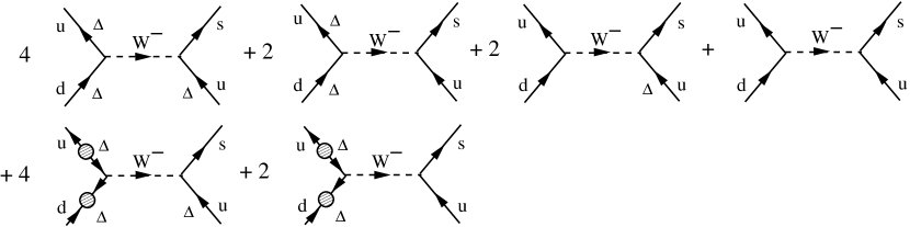
The collision integral is the sum of six terms, see Eq. (47), which are shown diagrammatically in Fig. 2 (in the same order as they appear in the equation). The superscripts at and in Eq. (47) correspond to the momenta in the order , , , , i.e., they describe the particles , , , , respectively, see diagrams in Fig. 1. The combinatorics of the process is constrained by color conservation for the vertices and . Consequently, and as well as and must have the same color. Hence, from Table 2 we conclude that and must be either both gapped () or both ungapped (). This can be seen in Fig. 2, where we have added the gap at the fermion line whenever the corresponding mode is gapped. It can also be seen in Eq. (47), where the pair of first and last superscripts is either (1,1) or (2,2). Furthermore, the second and third superscript can be (1,3) or (2,3), describing a (red or green) gapped and a (red or green) or a (blue) ungapped and a (blue) , respectively. The quark is ungapped for all colors. Combining these pairs and counting color degeneracies yields the six terms with respective prefactors in Eq. (47) and Fig. 2. In the cases where both and are gapped, there is an additional contribution from the anomalous propagators. This is denoted by in Eq. (47) and by a condensate insertion in Fig. 2. From the diagrams it is clear that there can be no condensate insertion for . This would lead to a violation of electric charge conservation at the vertex . Summarizing the result of the combinatorics, we have found that the process in the 2SC phase can be considered as composed of several subprocesses, where zero, one, two, or three of the participating particles have a gap in their excitation spectrum.
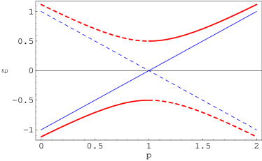
From Eqs. (50) and (51) we see that the process not only contains several subprocesses due to the 2SC pairing pattern, also every single of these subprocesses is written as a sum over 16 terms, expressed as a sum over . To understand the physical meaning of this sum, it is instructive to rewrite it and recover the unpaired phase limit. The change of variables described in the following is illustrated in Fig. 3. We may rewrite every single sum over by observing that for any function we have
| (53) |
where the new Bogoliubov coefficients and quasiparticle energies are defined as
| (54) |
Consequently, in Eqs. (50) and (51) we can replace by and by . Then, we obtain for the contribution from the normal propagators,
| (55) | |||||
and for the contribution of the anomalous propagators
| (56) | |||||
Because of for , only one of the 16 terms, namely , survives in the unpaired phase limit and we immediately obtain for this case
| (57) | |||||
in accordance with Ref. Madsen:1993xx . Note that in the representation of Eq. (50), all 16 subprocesses contribute even in the unpaired phase (of course yielding the same result (57)). It is easy to understand that the quantities in Eq. (54) are more natural to describe the unpaired phase because describes particle excitations for all momenta . In contrast, describes hole excitations for and particle excitations for . This distinction between particles and holes is not possible in the quasiparticle description of the superconducting phase. However, also in the 2SC phase the new representation is instructive since it reveals the processes that are only possible in a superconductor/superfluid, namely the 15 subprocesses that contain at least one . They correspond to processes in which three particles coalesce to one particle (or one particle decays into three) and in which four particles are annihilated (or created). This is possible because particle number is not conserved. Particles can be created from or deposited into the condensate. Only when there is no condensate, the “conventional” process of two incoming and two outgoing particles is the only possible one. In the next section, we shall study the quantitative contribution of these “exotic” processes to the total rate.
As a result of this subsection, let us rewrite the collision integral (47) using the following more illustrative notation,
| (58) |
where summation over the respective is implied. We shall also use the shorthand notation etc. where no confusion is possible. This notation shows explicitly how many gapped modes participate in the respective subprocesses. The definitions of the new quantities is clear from comparison with Eq. (47), the sum over , , originating from Eqs. (55) and (56). Since the quark (corresponding to ) is ungapped, only terms with survive, and the superscripts , , as well as the three arguments of the functions correspond to the quark flavors , , and . It is clear from the definition that the number of gapped modes determines how many of the 16 subprocesses are nonvanishing. This number can be directly read off from the notation in Eq. (58), i.e., all ’s that are shown explicitly have to be summed over , while the missing are set to , since the contribution for vanishes.
IV Evaluation of the rate
The general evaluation of the collision integral has to be done numerically. As a consistency check, let us derive the analytical result in the unpaired phase for zero temperature. In this case, all Fermi distributions in Eq. (57) become step functions,
| (59) | |||||
Since we assumed that , the second term in square brackets vanishes. (The first three step functions in this term imply which, for , contradicts the fourth one, implying .) Physically, this means that at zero temperature the process only happens in one direction. This direction is given by the sign of . The first term in square brackets can be evaluated upon using the definition of the function in Eq. (108a). One finds
| (60) | |||||
which is in agreement with Ref. Madsen:1993xx .
We treat all other cases numerically. For the following results we use MeV and MeV. We assume a transition temperature of MeV. Via the relation , where is the Euler-Mascheroni constant, this corresponds to a zero-temperature gap MeV. We shall employ the following model temperature dependence of the gap,
| (61) |
We have to compute the collision integrals for all combinations of , , shown in Eq. (58). Let us analyse the various subprocesses before we add them up to the total rate. To this end we pick the first term on the right-hand side of Eq. (58), which actually is a sum of 8 subrates. We show the rates of all 8 subprocesses of in Fig. 4. The figure shows that, due to symmetries of the collision integral, some of the resulting curves coincide. One obtains four groups, characterized by zero, one, two, and three factors in the collision integral (from top to bottom in the figure). In other words, the three lower curves in the right panel describe processes of coalescence or decay of particles, while the upper curve corresponds to a “normal” interaction process of two incoming and two outgoing particles. The left panel shows that this “normal” process is the only one that does not vanish at the transition temperature. Of course, all other processes can only contribute to the rate in the presence of a condensate. Although smaller in magnitude, these processes cannot be completely neglected for any temperature range since their contribution increases quickly for temperatures decreasing down from . A quantitative analysis shows that the seven processes where at least one of , , equals add up to about 30% of the total rate at , and their relative contribution increases monotonically with decreasing temperature.
An evaluation of the 8 subprocesses from Eq. (56), , shows that their contribution is of the order of the processes . Or, to give another quantitative estimate of these processes, we find that . Therefore, one can neglect these contributions, i.e., we may use for the almost identical rate .
For the rates and there are 4 and 2 subprocesses, respectively. We do not show the results for these subprocesses explicitly, since the corresponding plots are very similar to the ones in Fig. 4.
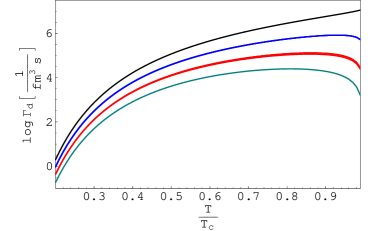
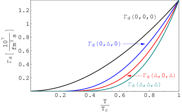
After having discussed the subprocesses for a given number of gapped fermions, we shall now compare the rates for processes with different numbers of gapped fermions. I.e., so far we have picked the first of the terms on the right-hand side of Eq. (58) and analyzed the subprocesses hidden in this term. Now we shall compare the different terms in this equation with each other. This is done in Fig. 5. Every curve in this figure corresponds to the rate of a given number of participating gapped fermions, where the number of gapped fermions increases from the top to the bottom curve. One sees that all rates containing at least one gapped fermion are strongly suppressed for small temperatures. This suppression can easily be extracted analytically, see Appendix E. For , the leading behavior for small temperatures is
| (62) |
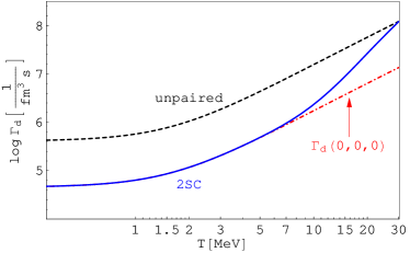
In Appendix E, also the behavior for , is derived (although this regime is not relevant in the present context). From the suppression due to the gap (62) we conclude that for small temperatures, we may approximate the total 2SC rate by the contribution of ungapped fermions, Madsen:1999ci . In Fig. 6 we see that this approximation starts to break down for temperatures .
V Results for the bulk viscosity
In this section, we compute the bulk viscosity of 2SC quark matter as a function of temperature. We first discuss the role of the subprocesses in Sec. V.1 before we compare the total bulk viscosity of the 2SC phase with that of unpaired quark matter in Sec. V.2. We make use of the expression for the bulk viscosity derived in Sec. II, see Eq. (21). This equation shows that we need the quantities , , , and . For the coefficients and , see definitions (10) and (14) and Table 1; we use a strange mass MeV and a chemical potential of MeV. In order to determine , we need the results for the rate , presented in the previous section. Remember that, in the derivation of the bulk viscosity, leading to Eq. (21), we have assumed the rate to be linear in , see Eq. (8). This linear approximation is, for any given temperature , valid for a sufficiently small . Physically, this means that we assume the volume oscillation to be sufficiently small, because the magnitude of is proportional to , see Eq. (19). Technically, we have to compute the rate at a sufficiently small such that we can determine , and thus the characteristic frequency , via . (Hence, we cannot necessarily use the numerical values from the previous section which have been obtained for a fixed MeV.)
V.1 Contribution of subprocesses to the bulk viscosity
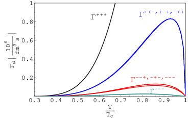
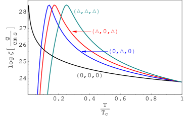
Before we turn to the final results for the 2SC phase, let us discuss the contribution of the subprocesses. As we have discussed in Sec. IV, the rates of the subprocesses depend on the number of gapped fermions that participate in the process. In Fig. 5 we have shown these rates, namely , , , and . In Fig. 7, we show four different bulk viscosities, assuming (fictitiously) that the bulk viscosity solely depends on each of these rates. The different suppression of the rates as a function of temperature leads to different temperatures at which the bulk viscosity becomes maximal (see Sec. V.2 for a further discussion of the maxima of the viscosity). What do we conclude for the 2SC bulk viscosity from these curves? Or, in other words, how do these curves “add up” to yield the total bulk viscosity as a function of temperature? To answer this question, remember the analogy between periodically expanding and contracting quark matter and an electric circuit with alternating voltage, see Sec. II. In that section we explained that one may think of a “capacitance” that behaves like the inverse of the rate , see Eq. (16). If the rate consists of a sum of several distinct subrates (as is the case in 2SC quark matter), small subrates can be neglected if there is a large, dominating subrate. The resulting “capacitance” is then determined by the dominating subrate, just as in an electric circuit with capacitors , in series where . Therefore, the bulk viscosity of 2SC quark matter is dominated by the subprocess of ungapped fermions, , although each of the subprocesses with gapped fermions would, for certain temperatures and in the absence of , yield a much larger bulk viscosity (as can be seen by comparing Fig. 7 with the final results, Fig. 8). Note that it is crucial for this argument that all subprocesses (all “capacitors”) affect one single chemical nonequilibrium (one single “current”), characterized by .
In Appendix B we show how this argument is altered when there is more than one independent . To illustrate this point let us assume for a moment that the strong interactions, which can change the color of the quarks, are no faster than the weak interactions. In this case, we must not consider the “accumulated” process , but nine processes , where and each stand for one of three colors, . And, importantly, there is not only a single , but nine ’s, one for each of these subprocesses. In this picture, the bulk viscosity is sensitive to the re-equilibration of each of the nine out-of-equilibrium quantities , leading to a significantly different result. Roughly speaking, the result would be a curve that follows all the maxima of the curves in Fig. 7. However, this picture is unphysical since it ignores the effect of the strong interactions. They provide color-changing processes on a time scale much faster than the weak processes. We show in Appendix B that, after taking into account the strong processes, one arrives at the simpler picture that has been used in Sec. II: There is only a single out-of-equilibrium quantity and the subrates add up like capacitors in series in an electric circuit. Then, the physical result for the total bulk viscosity is given by Fig. 8, which we discuss in the following.
V.2 Bulk viscosity of 2SC quark matter
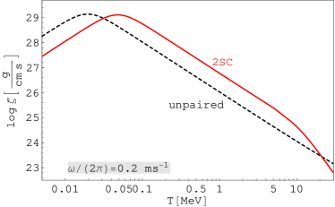
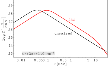
In Fig. 8 we show the bulk viscosity for unpaired and 2SC quark matter for two different oscillation frequencies (left panel) and (right panel). We now explain the features of these plots.
-
The bulk viscosity peaks at a particular temperature. This is expected from Eq. (21): the bulk viscosity as a function of the rate , for a fixed external frequency , has a maximum at , when the frequency of the externally imposed compression matches the microscopic equilibration rate. Since the microscopic rate is a monotonic function of the temperature (see results of the previous section), we see this maximum when we compute the bulk viscosity as a function of .
-
The peak viscosities are easily determined by setting in Eq. (21),
(63) i.e., they are independent of the microscopic equilibration rate. In particular, this simple relation explains the larger maximum values of the viscosity in the left panel of Fig. 8 compared to the right panel because of the different values of . In general, is different for unpaired and 2SC quark matter because the values of and differ from phase to phase, see Table 1. For the chosen values of and , the peak values happen to be almost identical.
-
The 2SC phase has its maximum viscosity at a higher temperature than the unpaired phase; near and above this temperature (up to ), the 2SC phase has a larger viscosity than the unpaired phase. This follows from the fact that is monotonically increasing, but the 2SC phase has a slower equilibration rate. At very low temperatures both rates are slow, and the higher rate is closer to , so the unpaired phase has higher viscosity Madsen:1999ci . At higher temperatures, both rates are above , but now the slower rate is closer to , so the 2SC phase has higher viscosity.
-
At low temperature, up to temperatures where the viscosity of the unpaired phase peaks, the unpaired and 2SC viscosities differ by a constant factor (the two lines are parallel on our logarithmic plot). This follows from for and the results of the previous section where we have shown that for sufficiently small temperatures, roughly (see Fig. 6), the rates simply differ by a factor 9 because the contribution of the gapped modes can be neglected. Also for temperatures larger than the temperature at which the viscosity of the 2SC phase peaks up to MeV, the viscosities differ by a constant factor. However, they are now in reversed order since for .
-
At the critical temperature, here chosen to be MeV, the rates of the two phases become the same (the 2SC gap vanishes). However, due to the “locking” of Fermi surfaces in the 2SC phase and the resulting difference in the coefficients entering the viscosity, the viscosities are different. From the values in Table 1 we conclude , in agreement with the results shown in Fig. 8.
VI Conclusions
We have computed the bulk viscosity of three-flavor color-superconducting quark matter in the 2SC phase originating from the nonleptonic weak process . To this end, we have presented a detailed calculation of the rate for this process for arbitrary temperatures. Since 2SC quark matter contains ungapped strange quarks as well as gapped and ungapped up and down quarks, this process contains several subprocesses. Each of these subprocesses that contains at least one gapped quasiparticle mode can be further divided into “subsubprocesses” which are similar to the ones in ordinary superfluids such as 3He. In both color superconductors and 3He, these subsubprocesses allow for creation and annihilation of quasiparticles from the condensate. Therefore, the process has contributions from decay and coalescence processes. We have presented a formal derivation of the total rate, starting from a kinetic equation and making use of the microscopic fermion propagators, resulting in an expression that naturally contains all these contributions. Our results are not only interesting for the special case of the 2SC phase but also, because of the multitude of subprocesses, provide a general quantitative analysis for the effect of a fermion condensate on the considered nonleptonic process.
We have evaluated the rate numerically, observing the expected exponential suppressions for small temperatures. For subprocesses with three gapped modes we find a suppression of the form , while two or one gapped mode(s) yield . Upon evaluating the collision integral for temperatures up to the superconducting transition temperature, we have also studied the temperature regime where the exponential functions are no longer valid approximations for the rate.
The results for the rate, which translate into a typical time scale of the weak process, have been used to compute the bulk viscosity as a function of temperature for a given external oscillation frequency, chosen to be of order 1 kHz, which corresponds to the fastest rotation rate observed for pulsars. We have pointed out that the bulk viscosity is the response of the quark system to this external oscillation just as an electric circuit responds to an external alternating voltage by an induced current. In this sense, we have identified a “resistance” and a “capacitance” of the quark system in terms of the microscopic process. Using this analogy, it is easy to understand that the behavior of the bulk viscosity assumes a maximum when the microscopic time scale matches that of the external frequency.
Our calculations show that, for a transition temperature of MeV and oscillation frequencies in the kHz range, the bulk viscosity of 2SC quark matter is larger than that of unpaired quark matter over a wide temperature range. This range is approximately given by for an oscillation period of one millisecond. For longer oscillation periods, this range is even larger. As discussed above, this is because in that temperature range the slower equilibration rate of 2SC matter resonates better with kHz frequency oscillations than does the faster equilibration rate of unpaired quark matter. This result has potential physical implications for the behavior of the star early in its life, before its internal temperature drops below about 0.1 MeV. It is also interesting to note that at these early times neutrinos are trapped, and the resultant lepton number chemical potential can favor a 2SC phase with strange quarks Steiner:2002gx (but see also Ruster:2005ib ). Moreover, bulk viscosity is likely to be the dominant factor for damping of potentially unstable -modes in this very temperature regime Kokkotas:2001ze ; Weber:2004kj . Although the star cools down below 0.1 MeV within days, this short time might potentially be long enough for instabilities to grow and spin down the star drastically Lindblom:2000az . For hot newly born stars, we have thus found that quark Cooper pairing actually works in favor of damping of unstable modes. For much smaller temperatures, keV, shear viscosity effects become important, and Cooper pairing is expected to reduce the shear viscosity and thus the damping of the unstable modes Madsen:1999ci . We have found a similar effect for the bulk viscosity: for sufficiently small temperatures, , the bulk viscosity of 2SC quark matter is smaller than that of unpaired quark matter. Besides the damping of unstable rotational modes, bulk viscosity is also an important quantity for time scales of radial pulsation of compact stars Sahu:2001iv . Our results can serve as an ingredient for calculations addressing the viscous damping of these pulsations.
Finally, we emphasize that the results for the bulk viscosity in the 2SC phase cannot be extrapolated to the CFL phase. In this phase, all fermions acquire a gap in their energy spectrum and thus the rate of the process will be smaller than in the 2SC phase. In particular, this rate will be exponentially suppressed for small temperatures. However, kaons (which have nonzero strangeness) serve as a more effective source for re-equilibration, and their contribution to the bulk viscosity has to be taken into account preparation .
Acknowledgements.
The authors like to thank M. Braby, P. Jaikumar, S. Reddy, D. Rischke, B. Sa’d, and I. Shovkovy for valuable discussions and acknowledge support by the U.S. Department of Energy under contracts #DE-FG02-91ER40628 and #DE-FG02-05ER41375 (OJI).Appendix A Bulk viscosity including leptonic processes
In this appendix, we derive an expression for the bulk viscosity which is valid for a system that not only converts into quarks via the non-leptonic process considered in the main part of the paper, but also contains leptonic processes. We shall consider the following three processes, employing the linear approximation for the several rates as in Sec. II,
| (64a) | |||||
| (64b) | |||||
| (64c) | |||||
The quantities , , and correspond to , , and in Sec. II. In chemical equilibrium, . Out of equilibrium, the quantities
| (65a) | |||||
| (65b) | |||||
| (65c) | |||||
are nonzero (we assume ). Note that there are only two independent ’s. According to the above microscopic processes, the densities for electrons and quarks change as follows,
| (66a) | |||||
| (66b) | |||||
| (66c) | |||||
| (66d) | |||||
We can thus express all density changes in terms of the changes in and . Analogous to Sec. II, we write the pressure as
| (67) | |||||
where
| (68a) | |||||
| (68b) | |||||
and we have made use of the relations between the various densities given in Eqs. (66). For the purpose of this appendix, it is sufficient to consider unpaired quark matter. In the 2SC phase, and would have additional terms due to the pairing of and quarks. Since the conclusions of this appendix do not depend on the values of and we may for simplicity proceed without taking into account the effects of pairing. Then, the average power dissipation, cf. Eq. (9), is
| (69) |
where we abbreviated
| (70a) | |||||
| (70b) | |||||
The changes in the chemical potentials are derived as in Sec. II, cf. Eqs. (11) and (12),
| (71) |
where
| (72a) | |||||
| (72b) | |||||
with
| (73a) | |||||
| (73b) | |||||
The single differential equation (12) thus has become a system of two coupled differential equations (71). With the ansatz we may reduce the system of differential equations to an algebraic set of four linear equations for the four variables , , , ,
| (74a) | |||||
| (74b) | |||||
From Eq. (69) and we conclude that only the real parts of the complex amplitudes enter the power dissipation. They are given by
| (75a) | |||||
| (75b) | |||||
Consequently, Eq. (69) and the definition (1) yield the bulk viscosity
| (76) |
where
| (77a) | |||||
| (77b) | |||||
| (77c) | |||||
| (77d) | |||||
With the densities (of unpaired quark matter) , , and we have
| (78a) | |||||
| (78b) | |||||
| (78c) | |||||
From the definitions it it clear that and correspond to and in Sec. II, respectively. The result (76) together with the definitions (77) shows that the three processes are entangled in a complicated way. Let us consider some limit cases in which the processes disentangle. In particular, we are interested in the case , since we expect the rates for the leptonic processes to be much smaller than the rate for the non-leptonic process. In this case,
| (79) |
In order to obtain some qualitative insight we have to compare the inverse time scale with the inverse time scales set by , , and . For simplicity, let us set . As a rough estimate, we shall assume that the factors containing one or several ’s all contribute by a factor , i.e., , . Then, the relevant inverse time scales
| (80) |
are, for fixed , indeed set solely by the corresponding rates of the non-leptonic and leptonic processes, respectively, and we can write
| (81) |
Obviously, it is incorrect to neglect the much slower process in general. Which process can be neglected rather depends on . In particular, we may consider several limit cases in which the time scales clearly separate, see Table 3. The general and plausible conclusion from this table is that the bulk viscosity is dominated by the process whose time scale is closest to the time scale set by the external oscillation. (Note that this is in contrast to subprocesses which contribute to one single , as considered in the main part of the paper. In this case, the fastest subprocess dominates the bulk viscosity even if there is a slower subprocess which, in the absence of the fast one, would produce a much larger bulk viscosity.) More specifically, the leptonic processes can be neglected in the high frequency limit (first row of Table 3) or when the frequency is close to the rate of the non-leptonic process (second row). When the frequency is smaller than the rate of the nonleptonic process, the leptonic processes can only be neglected if its rate is much smaller than the frequency and , i.e., if the frequency is much closer to the rate of the non-leptonic process than to the rate of the leptonic processes.
| order of time scales | |
|---|---|
Appendix B Bulk viscosity including strong processes
In this appendix, we show that the expression for the bulk viscosity derived in Sec. II is only correct in the presence of strong processes which are infinitely fast compared to the weak process . The treatment in Sec. II apparently simplifies the situation because the process in fact includes several combinations of quark colors. In principle, one has to treat all possible processes in a way analogous to the method presented in Appendix A, i.e., we have to consider the processes
| (82a) | |||||
| (82b) | |||||
| (82c) | |||||
| (82d) | |||||
| (82e) | |||||
| (82f) | |||||
| (82g) | |||||
| (82h) | |||||
| (82i) | |||||
As in Eqs. (64) we assign a rate to each of the processes and assume these rates to be proportional to the corresponding . There are nine different processes, because we can assign one of three colors (, , ) to each of the two (color-conserving) vertices of the process . From the results in Secs. III and IV we know that not all of the subprocesses have different rates. Due to the remaining color symmetry, we rather have four different rates depending on the number of gapped quasiparticles participating in the process. Using the notation introduced in Eq. (58), we have
| (83a) | |||||
| (83b) | |||||
| (83c) | |||||
| (83d) | |||||
However, for the purpose of this appendix we do not have to make any assumptions for the rates and may treat all nine rates, given by , as independent.
The various ’s can be written in terms of nine chemical potentials (one for each combination of color and flavor). It turns out that only five of them are independent,
| (84a) | |||||
| (84b) | |||||
| (84c) | |||||
| (84d) | |||||
| (84e) | |||||
| (84f) | |||||
| (84g) | |||||
| (84h) | |||||
| (84i) | |||||
We may thus choose , , , , , as independent variables. The density changes due to the above processes can be read off from Eqs. (82),
| (85a) | |||||
| (85b) | |||||
| (85c) | |||||
Obviously, the total change of the flavor density vanishes, while the total change of and flavor densities has the same absolute value but opposite signs,
| (86) |
where
| (87) |
If the bulk viscosity was determined solely by the above nine subprocesses of the weak process , we would have to set up a set of five coupled differential equations for the variables , , , , , analogous to Eq. (71). Its solution would yield the bulk viscosity through an equation analogous to Eq. (69). We have checked that this procedure would yield a result that differs from the one presented in Sec. V. In particular: While the bulk viscosity given by Eq. (21) is dominated by the fastest of the subprocesses (here ), the setup presented above would potentially allow all subprocesses to contribute significantly to the bulk viscosity (the dominant subprocesses would be determined by the external oscillation frequency ). In other words, this setup requires all chemical nonequilibria to re-equilibrate separately, and the one that resonates best with the external oscillation gives the largest contribution. In the remainder of this appendix, however, we show that this picture is invalidated by the presence of the strong interactions which allows the fermions to change their color on a much faster time scale than the one given by the weak interaction.
The relevant strong processes change the colors of two different quark flavors. Since there are three pairs of distinct flavors and three pairs of distinct colors, we have to consider the nine processes
| (88a) | |||||
| (88b) | |||||
| (88c) | |||||
Assuming these processes to be infinitely fast (this is equivalent to the assumption that the system be in chemical equilibrium with respect to all of these processes at any time) translates into the following conditions for the chemical potentials,
| (89a) | |||||
| (89b) | |||||
| (89c) | |||||
These equations result in four independent constraints. Consequently, we may express four chemical potentials in terms of the other five, e.g.,
| (90a) | |||||
| (90b) | |||||
Inserting these equations into Eqs. (84) reduces the number of independent ’s to one,
| (91) |
In order to set up the differential equation for this , we have to know the dependence of the densities on the remaining chemical potentials (after eliminating , , , via Eqs. (90)). Then, in the 2SC phase, the densities of the paired quarks , , , depend on the average chemical potential . The densities of the unpaired quarks are straightforwardly obtained with Eqs. (90). Let us, for simplicity, assume that . Then, we use the flavor densities from Eq. (87) to obtain
| (92) |
with given in Eq. (86). The same procedure is applied to the expression for the power dissipation, cf. Eq. (9). Upon using with defined in Eq. (8), we see that the final result is identical to Eq. (21). Consequently, we have proven that, due to (infinitely fast) strong processes, one can ignore the subtleties related to different ’s corresponding to subprocesses of . One rather may solely consider the rate which is the sum of the rates of these subprocesses and a single related to this rate. This is the method used in the main part of the paper.
Appendix C Dirac traces and contractions
From the definitions (34) and (43) we find
| (93a) | |||||
| (93b) | |||||
| (93c) | |||||
| (93d) | |||||
and
| (94a) | |||||
| (94b) | |||||
| (94c) | |||||
| (94d) | |||||
Consequently, we obtain the contractions
| (95a) | |||||
| (95b) | |||||
| (95c) | |||||
The imaginary terms in Eqs. (95b) and (95c) do not appear in the collision integral since they vanish after angular integration, see Appendix D.2.
Appendix D Angular integration
In the first part of this appendix we compute the angular integrals in Eqs. (48) and (49). In the second part we show that the angular integral over the imaginary terms in Eqs. (95b) and (95c) vanishes.
D.1 Angular integration in Eqs. (48) and (49)
We have to compute
| (96) |
One may start with the integral and rewrite the -function in terms of a modulus and an angular part
| (97) |
where stands for the angles of the vector . Thus, the effect of the angular -function is to replace the direction with (the numerator being actually because of the radial -function). Consequently, with we obtain
| (98) |
Next, we may straightforwardly perform the integration by choosing the -axis to be parallel to . As in Ref. wadhwa we denote
| (99) |
Then,
| (100) |
To obtain this result, note that . The remaining angular dependence is reduced to the angle between and , present in . Hence, one integration, say , is trivial while we are left with the azimuthal integral from ,
| (101) | |||||
Since , there are four orders of that yield nonvanishing integrals,
| (102a) | |||||
| (102b) | |||||
| (102c) | |||||
| (102d) | |||||
The two other possibilities, , and lead to vanishing integrals. Consequently,
| (103) |
where we defined
| (104) | |||||
with
| (105) | |||||
With a simple relabeling of momenta we obtain the result for the other two terms in Eq. (49),
| (106) |
and
| (107) |
Consequently, with the definitions
| (108a) | |||||
| (108b) | |||||
D.2 Angular integration over imaginary terms in Eqs. (95b) and (95c)
Here, we show that the integral
| (109) |
is zero. After integrating over one of the angles, say over , the scalar products containing a cross product can all be expressed in terms of one single scalar product,
| (110) |
Let’s consider the next integration, say over . The -function ensures that the distance of to a fixed vector, namely , equals a fixed value, namely . So all allowed vectors sit on a sphere around with radius . The value of the integrand is given by the projection of onto another fixed vector, namely . Since this vector is orthogonal to , the integral over all these projections vanishes.
For the formal proof, one uses a frame with -axis parallel to and an -axis parallel to (as above, ),
| (111) | |||||
because the integrand is odd in over the integration range.
Appendix E Rate for small temperatures
In this appendix, we determine the leading contribution for the rates , , at small temperatures. To this end, we analyse the following expression which originates from the Fermi distributions in the integrands of Eqs. (50) and (51) (prefactors are ignored since we only determine the leading contribution),
| (112) | |||||
where , , . This expression is integrated over , , , each ranging from to (the lower boundary actually being an approximation for ). We perform the sum and, for small (hence large ), approximate
| (113) | |||||
At this point, we distinguish between the different numbers of gapped modes. First, let us discuss the case . We expand and introduce the new (integration) variables ,
| (114) |
Now note that for sufficiently small , both and have the same temperature dependence,
| (115) |
Therefore, the limiting behavior of is different for the four cases , , , and . In particular, the latter case leads to a nonzero value of for . This can be seen from Eq. (114), where the 1 in the denominator of the fourth term on the right-hand side survives for . We show the results for all four cases in the first row of Table 4.
| 1 | ||||
| 1 | 1 | |||
| 1 | 1 | 1 | ||
| 1 | 1 | 1 | 1 |
References
- (1) J. C. Collins and M. J. Perry, Phys. Rev. Lett. 34, 1353 (1975).
- (2) D. Bailin and A. Love, Phys. Rept. 107, 325 (1984).
- (3) J. Bardeen, L.N. Cooper, and J.R. Schrieffer, Phys. Rev. 108, 1175 (1957).
- (4) For reviews, see K. Rajagopal and F. Wilczek, arXiv:hep-ph/0011333; M. G. Alford, Ann. Rev. Nucl. Part. Sci. 51, 131 (2001) [arXiv:hep-ph/0102047]; G. Nardulli, Riv. Nuovo Cim. 25N3, 1 (2002) [arXiv:hep-ph/0202037]; S. Reddy, Acta Phys. Polon. B 33, 4101 (2002) [arXiv:nucl-th/0211045]; T. Schäfer, arXiv:hep-ph/0304281; D. H. Rischke, Prog. Part. Nucl. Phys. 52, 197 (2004) [arXiv:nucl-th/0305030]; M. Alford, Prog. Theor. Phys. Suppl. 153, 1 (2004) [arXiv:nucl-th/0312007]; M. Buballa, Phys. Rept. 407, 205 (2005) [arXiv:hep-ph/0402234]; H. c. Ren, arXiv:hep-ph/0404074; M. Huang, Int. J. Mod. Phys. E 14, 675 (2005) [arXiv:hep-ph/0409167]; I. A. Shovkovy, Found. Phys. 35, 1309 (2005) [arXiv:nucl-th/0410091]. T. Schäfer, arXiv:hep-ph/0509068.
- (5) M. G. Alford, K. Rajagopal and F. Wilczek, Nucl. Phys. B 537, 443 (1999) [arXiv:hep-ph/9804403].
- (6) K. Rajagopal and A. Schmitt, Phys. Rev. D 73, 045003 (2006) [arXiv:hep-ph/0512043].
- (7) T. Schäfer, Phys. Rev. D 62, 094007 (2000) [arXiv:hep-ph/0006034]; M. Buballa, J. Hosek and M. Oertel, Phys. Rev. Lett. 90, 182002 (2003) [arXiv:hep-ph/0204275]; A. Schmitt, Q. Wang and D. H. Rischke, Phys. Rev. D 66, 114010 (2002) [arXiv:nucl-th/0209050]; M. G. Alford, J. A. Bowers, J. M. Cheyne and G. A. Cowan, Phys. Rev. D 67, 054018 (2003) [arXiv:hep-ph/0210106]; A. Schmitt, Ph.D. dissertation, arXiv:nucl-th/0405076; A. Schmitt, Phys. Rev. D 71, 054016 (2005) [arXiv:nucl-th/0412033].
- (8) M. G. Alford, J. A. Bowers and K. Rajagopal, Phys. Rev. D 63, 074016 (2001) [arXiv:hep-ph/0008208]; I. Giannakis and H. C. Ren, Phys. Lett. B 611, 137 (2005) [arXiv:hep-ph/0412015]; R. Casalbuoni, R. Gatto, N. Ippolito, G. Nardulli and M. Ruggieri, Phys. Lett. B 627, 89 (2005) [Erratum-ibid. B 634, 565 (2006)] [arXiv:hep-ph/0507247]; M. Mannarelli, K. Rajagopal and R. Sharma, Phys. Rev. D 73, 114012 (2006) [arXiv:hep-ph/0603076]; K. Rajagopal and R. Sharma, arXiv:hep-ph/0606066.
- (9) M. G. Alford, J. Berges and K. Rajagopal, Nucl. Phys. B 571, 269 (2000) [arXiv:hep-ph/9910254]; A. Schmitt, Q. Wang and D. H. Rischke, Phys. Rev. Lett. 91, 242301 (2003) [arXiv:nucl-th/0301090]; A. Schmitt, Q. Wang and D. H. Rischke, Phys. Rev. D 69, 094017 (2004) [arXiv:nucl-th/0311006].
- (10) E. J. Ferrer, V. de la Incera and C. Manuel, Phys. Rev. Lett. 95, 152002 (2005) [arXiv:hep-ph/0503162]; E. J. Ferrer, V. de la Incera and C. Manuel, Nucl. Phys. B 747, 88 (2006) [arXiv:hep-ph/0603233].
- (11) I. A. Shovkovy and P. J. Ellis, Phys. Rev. C 66, 015802 (2002) [arXiv:hep-ph/0204132].
- (12) G. W. Carter and S. Reddy, Phys. Rev. D 62, 103002 (2000) [arXiv:hep-ph/0005228]; P. Jaikumar, M. Prakash and T. Schäfer, Phys. Rev. D 66, 063003 (2002) [arXiv:astro-ph/0203088]; S. Reddy, M. Sadzikowski and M. Tachibana, Nucl. Phys. A 714, 337 (2003) [arXiv:nucl-th/0203011]; J. Kundu and S. Reddy, Phys. Rev. C 70, 055803 (2004) [arXiv:nucl-th/0405055]; R. Anglani, M. Mannarelli, G. Nardulli and M. Ruggieri, arXiv:hep-ph/0607341.
- (13) P. Jaikumar, C. D. Roberts and A. Sedrakian, Phys. Rev. C 73, 042801 (2006) [arXiv:nucl-th/0509093].
- (14) A. Schmitt, I. A. Shovkovy and Q. Wang, Phys. Rev. D 73, 034012 (2006) [arXiv:hep-ph/0510347].
- (15) Q. Wang, Z. g. Wang and J. Wu, arXiv:hep-ph/0605092.
- (16) B. A. Sa’d, I. A. Shovkovy and D. H. Rischke, arXiv:astro-ph/0607643.
- (17) A. Drago, A. Lavagno and G. Pagliara, Phys. Rev. D 71, 103004 (2005) [arXiv:astro-ph/0312009].
- (18) M. Alford and K. Rajagopal, JHEP 0206, 031 (2002) [arXiv:hep-ph/0204001].
- (19) A. W. Steiner, S. Reddy and M. Prakash, Phys. Rev. D 66, 094007 (2002) [arXiv:hep-ph/0205201].
- (20) S. B. Rüster, V. Werth, M. Buballa, I. A. Shovkovy and D. H. Rischke, Phys. Rev. D 72, 034004 (2005) [arXiv:hep-ph/0503184].
- (21) H. Abuki and T. Kunihiro, Nucl. Phys. A 768, 118 (2006) [arXiv:hep-ph/0509172].
- (22) C. Manuel, A. Dobado and F. J. Llanes-Estrada, JHEP 0509, 076 (2005) [arXiv:hep-ph/0406058].
- (23) K. D. Kokkotas and N. Andersson, arXiv:gr-qc/0109054.
- (24) N. Andersson, Astrophys. J. 502, 708 (1998) [arXiv:gr-qc/9706075];
- (25) N. Andersson and G. L. Comer, Mon. Not. Roy. Astron. Soc. 328, 1129 (2001) [arXiv:astro-ph/0101193].
- (26) For a lecture on r-mode instabilities see L. Lindblom, arXiv:astro-ph/0101136.
- (27) F. Weber, Prog. Part. Nucl. Phys. 54, 193 (2005) [arXiv:astro-ph/0407155]; F. Weber, A. Torres i Cuadrat, A. Ho and P. Rosenfield, PoS JHW2005, 018 (2006) [arXiv:astro-ph/0602047].
- (28) C. Cutler and L. Lindblom, Astrophys. J. 314, 234 (1987); R. F. Sawyer, Phys. Rev. D 39, 3804 (1989).
- (29) Q. D. Wang and T. Lu, Phys. Lett. B 148, 211 (1984).
- (30) P. Arnold, C. Dogan and G. D. Moore, arXiv:hep-ph/0608012.
- (31) P. Bhattacharyya, C.J. Pethick and H. Smith, Phys. Rev. B 15, 3367 (1977); C.J. Pethick, P. Bhattacharyya and H. Smith, Phys. Rev. B 15, 3384 (1977).
- (32) D. Vollhardt and P. Wölfle, The Superfluid Phases of Helium 3 (Taylor & Francis, London, 1990).
- (33) J. Madsen, Phys. Rev. D 46, 3290 (1992).
- (34) J. D. Anand, N. Chandrika Devi, V. K. Gupta and S. Singh, Pramana 54, 737 (2000).
- (35) P. Haensel, K. P. Levenfish and D. G. Yakovlev, Astron. Astrophys. 357, 1157 (2000) [arXiv:astro-ph/0004183].
- (36) L. Lindblom and B. J. Owen, Phys. Rev. D 65, 063006 (2002) [arXiv:astro-ph/0110558].
- (37) L. P. Kadanoff and G. Baym, Quantum Statistical Mechanics (Benjamin, New York, 1962).
- (38) M. Schönhofen, M. Cubero, B. L. Friman, W. Nörenberg and G. Wolf, Nucl. Phys. A 572, 112 (1994).
- (39) A. Sedrakian and A. Dieperink, Phys. Lett. B 463, 145 (1999) [arXiv:nucl-th/9905039].
- (40) A. Wadhwa, V.K. Gupta, S. Singh, and J.D. Anand, J. Phys. G 9, 1137 (1995).
- (41) J. Madsen, Phys. Rev. D 47, 325 (1993).
- (42) J. Madsen, Phys. Rev. Lett. 85, 10 (2000) [arXiv:astro-ph/9912418].
- (43) S. B. Ruster, V. Werth, M. Buballa, I. A. Shovkovy and D. H. Rischke, Phys. Rev. D 73, 034025 (2006) [arXiv:hep-ph/0509073].
- (44) L. Lindblom, J. E. Tohline and M. Vallisneri, Phys. Rev. Lett. 86, 1152 (2001) [arXiv:astro-ph/0010653].
- (45) P. K. Sahu, G. F. Burgio and M. Baldo, Astrophys. J. 566, L89 (2002) [arXiv:astro-ph/0111414]; P. Haensel, K. P. Levenfish and D. G. Yakovlev, Astron. Astrophys. 394, 213 (2002) [arXiv:astro-ph/0208078]; M. E. Gusakov, D. G. Yakovlev and O. Y. Gnedin, Mon. Not. Roy. Astron. Soc. 361, 1415 (2005) [arXiv:astro-ph/0502583].
- (46) M. Alford, M. Braby, S. Reddy, T. Schäfer, in preparation.