Covariant theory of particle-vibrational coupling and its effect on the single-particle spectrum

Abstract

The Relativistic Mean Field (RMF) approach describing the motion of independent particles in effective meson fields is extended by a microscopic theory of particle vibrational coupling. It leads to an energy dependence of the relativistic mass operator in the Dyson equation for the single-particle propagator. This equation is solved in the shell-model of Dirac states. As a result of the dynamics of particle-vibrational coupling we observe a noticeable increase of the level density near the Fermi surface. The shifts of the single-particle levels in the odd nuclei surrounding ²⁰⁸Pb and the corresponding distributions of the single-particle strength are discussed and compared with experimental data.

I Introduction

New experimental facilities with radioactive nuclear beams make it possible to investigate the nuclear chart not only along the narrow line of stable isotopes but also in areas of large neutron- and proton excess far from the valley $\beta$-stability. This situation has stimulated enhanced efforts on the theoretical side to understand the dynamics of the nuclear many-body problem by microscopic methods. Very light nuclei with $A\leq 12$ are studied by an “ab initio” approach utilizing bare nucleon-nucleon interactions of  two- and three-body character and modern shell-model calculations based on large scale diagonalization techniques and truncation schemes show considerable success in predicting properties of somewhat heavier nuclei. For the large majority of nuclei, however, a quantitative microscopic description is only possible by density functional theory. These methods are based on mean-field theory. Although density functional theory can, in principle, provide an exact description of the many-body dynamics, if  the exact density functional is known, in nuclear physics one is far from a microscopic derivation of this functional. The most successful schemes use a phenomenological ansatz incorporating  as many symmetries of the system as possible and adjust the parameters of these functionals to ground state properties of characteristic nuclei all over the periodic table. Considerable progress has been reported recently in constructing such functionals. For a recent review see BHR.03 .

Of particular interest are covariant density functionals Rin.96 ; VALR.05 because they are based on Lorentz invariance. This symmetry not only allows to describe the spin-orbit coupling, which has an essential influence on the underlying shell structure, in a consistent way, but it also put stringent considerable restrictions on the number of parameters in the corresponding functionals without reducing the quality of the agreement with experimental data. A very successful example is the Relativistic Hartree-Bogoliubov model RHB . It combines a density dependence through a non-linear coupling between the meson fields BB.77 with pairing correlations based on an effective interaction of finite range. A large variety of nuclear phenomena have been described over the years within this model: the equation of state in symmetric nuclear matter, ground state properties of finite spherical and deformed nuclei all over the periodic table GRT.90 from light nuclei LVR.04a to super-heavy elements LSRG.96 , from the neutron drip line, where halo phenomena are observed MR.96 to the proton drip line LVR.04 with nuclei unstable against the emission of protons LVR.99 . Recently this model has been also applied very successfully for the description of excited states, such as rotational bands in normal and super-deformed nuclei AKRE.00 ; ARK.00 and collective vibrations MWG.02 . Rotations are treated in the cranking approximation, which provides a quasi-static description of the nuclear dynamics in a rotating frame and for the description of vibrations a time-dependent mean field approximation is used by assuming independent particle motion in time-dependent average fields VBR.95 . In the small amplitude limit one obtains the relativistic Random Phase Approximation (RRPA) RMG.01 . This method provides a natural framework to investigate collective and non-collective excitations of $ph$-character. It is successful in particular for the understanding of the position of giant resonances and spin- or/and isospin-excitations as the Gamov Teller Resonance (GTR) or the Isobaric Analog Resonance (IAR). Recently it has been also used for a theoretical interpretation of  low-lying E1-strengths observed in neutron rich isotopes (pygmy modes) PRN.03 and for low-lying collective quadrupole excitations Ans.05 .

Of course the density functional theory based on the mean field framework cannot provide an exact treatment of the full nuclear dynamics. It is known to break down not only in transitional nuclei, where one has to include correlations going beyond the mean field approximation by treating quantum fluctuations through a superposition of several mean field solutions, as for instance in the Generator Coordinate Method (GCM) RS.80 , but already in ideal shell model nuclei such as ²⁰⁸Pb with closed protons and neutron shells one finds in self-consistent mean field calculations usually a single particle spectrum with a considerably enhanced Hartree-Fock gap in the spectrum and a reduced level density at the Fermi surface as compared with the experiment. It is well known that this fact is connected with the relatively small effective mass in such models.

Mahaux and collaborators JLM.76 have shown that the effective mass in nuclear matter is roughly $m^{\ast}/m$ $\approx 0.8$. In finite nuclei it should be modified by the coupling of the single particle motion to low-lying collective surface vibrations. This leads, in the vicinity of the Fermi surface, to an enhancement of $m^{\ast}/m$ $\approx 1$. Non-self-consistent models with the bare mass ( $m^{\ast}/m$ $\approx 1$) show indeed a single particle spectrum with a level density close to the experiment.

Using the quasi-particle concept of Landau theory and Green’s function techniques, one can derive a one-body equation for the single-particle Green’s function, which is in principle exact, the Dyson equation Mig.67 . It contains a non-local and energy dependent self-energy, also called mass-operator. The energy independent part of this operator can be described very well in mean field theory. The most important origin of an energy dependence is given by the coupling of the single particle motion to low-lying collective vibrations.

II The energy dependent part of the mass operator

II.1 One-nucleon motion in the relativistic mean field

In the relativistic nuclear theory the motion of the nucleons is described by the Dirac equation

$$\bigl{(}\gamma^{\mu}P_{\mu}-m^{\ast}\bigr{)}|\psi\rangle=0,$$ (1)

where the effective mass is given by

$$m^{\ast}=m+\Sigma_{s}$$ (2)

with the scalar part $\Sigma_{s}$ of the mass operator and where the generalized four-vector momentum operator has the form

$$P_{\mu}=p_{\mu}-\Sigma_{\mu}=\Bigl{(}i\frac{\partial}{\partial t}-\Sigma_{0},i\mathbf{\nabla}+\mathbf{\Sigma}\Bigr{)}$$ (3)

with the vector part $\Sigma^{\mu}$ of the mass operator

$$\Sigma^{\mu}=(\Sigma^{0},\mathbf{\Sigma}).$$ (4)

The index ’$s$’ in the Eq. (2) denotes that the effective mass is described by the scalar $\sigma$-meson field. In order to characterize ground state properties the stationary Dirac equation has to be solved:

$$\bigl{(}{\mbox{\boldmath$\alpha$}}(\mathbf{p}-\mathbf{\Sigma})+\beta m^{\ast}+\Sigma_{0}\bigr{)}|\psi\rangle=\varepsilon|\psi\rangle.$$ (5)

In the general case the full mass operator is non-local in the space coordinates and also in time. This non-locality means that its Fourier transform has both momentum and energy dependence. Let us assume the components of mean field to be sums of the stationary local and energy dependent non-local terms:

$$\Sigma(\mathbf{r},\mathbf{r^{\prime}};\omega)={\tilde{\Sigma}}(\mathbf{r})\delta(\mathbf{r}-\mathbf{r^{\prime}})+\Sigma^{e}(\mathbf{r},\mathbf{r^{\prime}};\omega),$$ (6)

where all the components of the mass operator are involved:

$${\Sigma}=({\Sigma}_{s},{\Sigma}^{\mu})$$

$$\tilde{\Sigma}=(\tilde{\Sigma}_{s},\tilde{\Sigma}^{\mu})$$

$${\Sigma}^{e}=({\Sigma}_{s}^{e},{\Sigma}^{e\mu})$$ (7)

and index ”e” indicates the energy dependence.

The scalar component of the energy-independent mass operator is proportional to the $\sigma$-meson field:

$${\tilde{\Sigma}}_{s}(\mathbf{r})=g_{\sigma}\sigma(\mathbf{r}).$$ (8)

Time-like and space-like components of the local and energy-independent part of the mass operator ($\tilde{\Sigma}^{\mu}$) are generated by the isoscalar $\omega$-meson and isovector $\rho$-meson fields $\omega^{\mu},{\vec{\rho}}^{\ \mu}$ and Coulomb field $A^{\mu}$:

$${\tilde{\Sigma}}^{\mu}(\mathbf{r})=g_{\omega}\omega^{\mu}(\mathbf{r})+g_{\rho}{\vec{\tau}}{\vec{\rho}}^{\ \mu}(\mathbf{r})+e\frac{(1-\tau_{3})}{2}A^{\mu}(\mathbf{r}),$$ (9)

where arrows denote isovectors and bold-faced letters indicate vectors in three-dimensional space. These fields satisfy the inhomogeneous Klein-Gordon equations:

$$(-\Delta+m_{\sigma}^{2})\ \sigma(\mathbf{r}) =-g_{\sigma}\rho_{s}(\mathbf{r})-g_{2}\sigma^{2}(\mathbf{r})-g_{3}\sigma^{3}(\mathbf{r})$$ (10)

$$(-\Delta+m_{\omega}^{2})\ \omega^{\mu}(\mathbf{r}) =g_{\omega}j^{\mu}(\mathbf{r})$$ (11)

$$(-\Delta+m_{\rho}^{2})\ {\vec{\rho}}^{\ \mu}(\mathbf{r}) =g_{\rho}{\vec{j}}^{\ \mu}(\mathbf{r})$$ (12)

$$-\Delta A^{\mu}(\mathbf{r}) =ej_{p}^{\mu}(\mathbf{r}),$$ (13)

where the sources are determined by the respective density and current distributions in a system of A nucleons: the scalar density for $\sigma$-field

$$\rho_{s}(\mathbf{r})=\sum\limits_{i=1}^{A}{\bar{\psi}}_{i}(\mathbf{r})\psi_{i}(\mathbf{r}),$$ (14)

the baryon current for the $\omega$-field

$$j^{\mu}(\mathbf{r})=\sum\limits_{i=1}^{A}{\bar{\psi}}_{i}(\mathbf{r})\gamma^{\mu}\psi_{i}(\mathbf{r}),$$ (15)

the isovector current for the $\rho$-field

$${\vec{j}}^{\ \mu}(\mathbf{r})=\sum\limits_{i=1}^{A}{\bar{\psi}}_{i}(\mathbf{r})\gamma^{\mu}{\vec{\tau}}\psi_{i}(\mathbf{r}),$$ (16)

and the charge current for the photon-field

$$j_{p}^{\mu}(\mathbf{r})=\sum\limits_{i=1}^{Z}{\bar{\psi}}_{i}(\mathbf{r})\gamma^{\mu}\frac{(1-\tau_{3})}{2}\psi_{i}(\mathbf{r}).$$ (17)

The summation in (14 – 16) is performed over occupied states in the Fermi sea, in accordance with no-sea approximation, so that the contribution of the negative-energy states to the densities and currents is neglected.

II.2 The single-particle Green’s function

In the present work we assume time-reversal symmetry that means the absence of currents in the nucleus and, thus, vanishing space-like components of $\ {\Sigma}$. The equation of the one-nucleon motion has the form:

$$\bigl{(}h^{\mathcal{D}}+\beta\Sigma_{s}^{e}(\varepsilon)+\Sigma_{0}^{e}(\varepsilon)\bigr{)}|\psi\rangle=\varepsilon|\psi\rangle$$ (18)

or, in the language of Green’s functions

$$\bigl{(}\varepsilon-h^{\mathcal{D}}-\beta\Sigma_{s}^{e}(\varepsilon)-\Sigma_{0}^{e}(\varepsilon)\bigr{)}G(\varepsilon)=1,$$ (19)

where $h^{\mathcal{D}}$ denotes the Dirac hamiltonian with the energy-independent mean field:

$$h^{\mathcal{D}}={\mbox{\boldmath$\alpha$}}\mathbf{p}+\beta(m+{\tilde{\Sigma}}_{s})+{\tilde{\Sigma}}_{0}.$$ (20)

We now work in the shell-model Dirac basis $\{|\psi_{k}\rangle\}$ which diagonalizes the energy-independent part of the Dirac equation:

$$h^{\mathcal{D}}|\psi_{k}\rangle=\varepsilon_{k}|\psi_{k}\rangle.$$ (21)

In addition we assume in the present work spherical symmetry. In this case the spinor $|\psi_{k}\rangle$ is characterized by the set of single-particle quantum numbers $k=\{(k),m_{k}\},(k)=\{t_{k},\pi_{k},n_{k},j_{k},l_{k}\}$ with the radial quantum number $n_{k}$, angular momentum quantum numbers $j_{k},m_{k}$, parity $\pi_{k}$ and isospin $t_{k}$:

$$\psi_{k}(\mathbf{r},s,t)=\left(\begin{array}[c]{c}f_{(k)}(r)\Phi_{l_{k}j_{k}m_{k}}(\vartheta,\varphi,s)\\ ig_{(k)}(r)\Phi_{{\tilde{l}}_{k}j_{k}m_{k}}(\vartheta,\varphi,s)\end{array}\right)\chi_{t_{k}}(t),$$ (22)

where the orbital angular momenta $l_{k}$ and $\tilde{l}_{k}$ of the large and small components are determined by the parity of the state $k$:

$$\left\{\begin{array}[c]{ccc}l_{k}=j_{k}+\frac{1}{2},&{\tilde{l}}_{k}=j_{k}-\frac{1}{2}&\mbox{for}\ \ \pi_{k}=(-1)^{j_{k}+\frac{1}{2}}\\ l_{k}=j_{k}-\frac{1}{2},&{\tilde{l}}_{k}=j_{k}+\frac{1}{2}&\mbox{for}\ \ \pi_{k}=(-1)^{j_{k}-\frac{1}{2}},\end{array}\right.$$ (23)

$f_{(k)}(r)$ and $g_{(k)}(r)$ are radial wave functions and $\Phi_{ljm}$ is a two-dimensional spinor:

$$\Phi_{ljm}(\vartheta,\varphi,s)=\sum\limits_{m_{s}m_{l}}({\frac{{\scriptstyle 1}}{{\scriptstyle 2}}}m_{s}lm_{l}|jm)Y_{lm_{l}}(\vartheta,\varphi)\chi_{m_{s}}(s).$$ (24)

In this basis one can rewrite Eq. (19) as follows:

$$\sum\limits_{l}\bigl{\{}(\varepsilon-\varepsilon_{k})\delta_{kl}-\Sigma_{kl}^{e}(\varepsilon)\bigr{\}}G_{lk^{\prime}}(\varepsilon)=\delta_{kk^{\prime}},$$ (25)

where the letter indices $k,k^{\prime},l$ denote full sets of the spherical quantum numbers mentioned above.

In the next step we represent the exact single-particle Green’s function entering Eq. (19) in the Lehmann expansion. In contrast to the non-relativistic case, where one has occupied states below the Fermi surface (hole states $h$) and empty states above the Fermi surface (particle states $p$) we now have according to the no-sea approximation in addition empty states with negative energies (antiparticle states $\alpha$). For a detailed discussion of this point see also Ref. RMG.01 . Therefore the Lehmann representation of the Green’s function has the form

$$G_{kl}(\varepsilon)=\sum\limits_{h}\frac{\chi_{k}^{h0}\chi_{l}^{h0\ast}}{\varepsilon-\varepsilon_{h}-i\eta}+\sum\limits_{p}\frac{\chi_{k}^{0p}\chi_{l}^{0p\ast}}{\varepsilon-\varepsilon_{p}+i\eta}+\sum\limits_{\alpha}\frac{\chi_{k}^{0\alpha}\chi_{l}^{0\alpha\ast}}{\varepsilon-\varepsilon_{\alpha}+i\eta},$$ (26)

where $\eta\rightarrow+0$ and the matrix elements are defined as

$$\chi_{k}^{h0}=\langle h|{\hat{\psi}}_{k}|0\rangle,$$

$$\chi_{k}^{0p}=\langle 0|{\hat{\psi}}_{k}|p\rangle,$$

$$\chi_{k}^{0\alpha}=\langle 0|{\hat{\psi}}_{k}|\alpha\rangle.$$ (27)

Here ${\hat{\psi}}_{k}$ is the Dirac field annihilation operator of the state $k$. $|0\rangle$ denotes the ground state of the subsystem of $N$ particles in the even-even nucleus in no-sea approximation, i.e. the negative energy states are essentially empty. The states $|h\rangle$ correspond to the ground state and to excited states of the subsystem of ($N-1$) particles and $|p\rangle$ are the ground and excited states of the system of ($N+1$) particles, respectively. Because of the no-sea approximation the negative energy states $|\alpha\rangle$ are not occupied in $|0\rangle$ and therefore there exist also states $|\alpha\rangle$ in the ($N+1$) particle system where a level with negative energy are occupied.

II.3 The pole structure of the mass operator

Let us now define the energy-dependent part of the mass operator (simply called ’mass operator’ in the following). Its matrix elements have the form:

$$\Sigma_{kl}^{e}(\varepsilon)=\int d^{3}rd^{3}{r}^{\prime}~{}{\psi}_{k}^{+}(\mbox{\boldmath$r$})\bigl{(}\beta\Sigma_{s}^{e}({\mbox{\boldmath$r$}},{\mbox{\boldmath$r$}^{\prime}};\varepsilon)+\Sigma_{0}^{e}({\mbox{\boldmath$r$}},{\mbox{\boldmath$r$}^{\prime}};\varepsilon)\bigr{)}\psi_{l}({\mbox{\boldmath$r$}^{\prime}}).$$ (28)

Obviously, on this stage one needs some model assumptions. In the present work we choose a rather simple particle-phonon coupling model BM.75 to describe the energy dependence of $\Sigma^{e}$. Within this model $\Sigma^{e}$ is a convolution of the particle-phonon coupling amplitude $\Gamma$ and the exact single-particle Green’s function KT.86 :

$$\Sigma_{kl}^{e}(\varepsilon)=\sum\limits_{k^{\prime}l^{\prime}}\int\limits_{-\infty}^{+\infty}\frac{d\omega}{2\pi i}\Gamma_{kl^{\prime}lk^{\prime}}(\omega)G_{k^{\prime}l^{\prime}}(\varepsilon+\omega),$$ (29)

where the amplitude $\Gamma$ has the following spectral expansion

$$\Gamma_{kl^{\prime}lk^{\prime}}(\omega)=-\sum\limits_{\mu}\Bigl{(}\frac{\gamma_{k^{\prime}k}^{\mu\ast}\gamma_{l^{\prime}l}^{\mu}}{\omega-\Omega^{\mu}+i\eta}-\frac{\gamma_{kk^{\prime}}^{\mu}\gamma_{ll^{\prime}}^{\mu\ast}}{\omega+\Omega^{\mu}-i\eta}\Bigr{)}$$ (30)

in terms of phonon vertexes $\gamma^{\mu}$ and their frequencies $\Omega^{\mu}$. They are determined by the following relation:

$$\gamma_{kl}^{\mu}=\sum\limits_{k^{\prime}l^{\prime}}V_{kl^{\prime}lk^{\prime}}\delta\rho^{\mu}_{k^{\prime}l^{\prime}}.$$ (31)

$V_{kl^{\prime}lk^{\prime}}$ denotes the relativistic matrix element of the residual interaction and $\delta\rho$ is the transition density. In the present work we use the linearized version of the model which assumes that $\delta\rho$ is not influenced by the particle-phonon coupling and can be computed within relativistic RPA. The linearized version implies also that the energy-dependent part of the mass operator (28) contains the mean field Green’s function ${\tilde{G}}(\varepsilon)=(\varepsilon-h^{\mathcal{D}})^{-1}$ instead of the exact Green’s function $G$. So, the equation (25) becomes linear with respect to $G$. Since the mean field Green’s function is

$${\tilde{G}}_{kl}(\varepsilon)=\frac{\delta_{kl}}{\varepsilon-\varepsilon_{k}+i\sigma_{k}\eta},$$ (32)

where $\sigma_{k}=+1$ if $k$ is an unoccupied state of $p$- or $\alpha$-types and $\sigma_{k}=-1$ for an occupied $k$ states of $h$-type, the mass operator $\Sigma^{e}$ takes the form:

$$\Sigma_{kl}^{e}(\varepsilon)=\frac{\delta_{j_{k}j_{l}}\delta_{l_{k}l_{l}}}{2j_{k}+1}\sum\limits_{\mu,n}\frac{\langle k\parallel\gamma^{\mu(\sigma_{n})}\parallel n\rangle\langle l\parallel\gamma^{\mu(\sigma_{n})}\parallel n\rangle^{\ast}}{\varepsilon-\varepsilon_{n}-\sigma_{n}(\Omega^{\mu}-i\eta)}\ .$$ (33)

Here we use the notation:

$$\langle k\parallel\gamma^{\mu(\sigma_{n})}\parallel n\rangle=\delta_{\sigma_{n},1}\langle k\parallel\gamma^{\mu}\parallel n\rangle\ +\ \delta_{\sigma_{n},-1}\langle n\parallel\gamma^{\mu}\parallel k\rangle^{\ast}.$$ (34)

Since the indexes $k,l$ and $n$ run through the whole Dirac basis, each state in (33) can be a particle above the Fermi surface, a hole below the Fermi surface or a particle in a state with negative energy (antiparticle state). The graphical representation of the mass operator is given in Fig. 1. We draw the particle and the hole components assuming all the possible types of intermediate states. Solid line with arrow denotes a particle (hole) in the Fermi sea, dashed line means a particle in the empty Dirac sea, weavy line is a phonon propagator, and small circle denotes a phonon vertex (31). Time direction is from the left to the right.

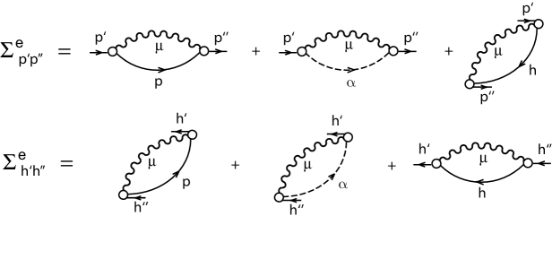
Figure 1: The particle $\Sigma^{e}_{p^{\prime}p^{\prime\prime}}$ and the hole $\Sigma^{e}_{h^{\prime}h^{\prime\prime}}$ components of the relativistic mass operator in the graphical representation. p, $\alpha$, h are the particle, antiparticle and hole types of the intermediate states. See text for the detailed explanation.

One can see from the Eq. (33) that the matrix $\Sigma_{kl}^{e}$ contains a small number of the off-diagonal elements with relatively large energy denominators. Additionally, it was shown by explicit calculations within the non-relativistic approach RW.73 that it is justified to use the diagonal approximation:

$$\Sigma_{kl}^{e}(\varepsilon)=\delta_{kl}\Sigma^{e}_{k}(\varepsilon)$$ (35)

with

$$\Sigma_{k}^{e}(\varepsilon)=\frac{1}{2j_{k}+1}\sum\limits_{\mu,n}\frac{|\langle k\parallel\gamma^{\mu(\sigma_{n})}\parallel n\rangle|^{2}}{\varepsilon-\varepsilon_{n}-\sigma_{n}(\Omega^{\mu}-i\eta)}\ .$$ (36)

In analogy with the conventional terminology of non-relativistic approaches, let us call the intermediate term $n$ ’polarization term’ if $\sigma_{n}=\sigma_{k}$ and ’correlation term’ if $\sigma_{n}=-\sigma_{k}$. The correlation term describes, obviously, the backwards going diagrams in Feynman’s language and corresponds to the ground state correlations caused by the particle-vibration coupling.

Thus, within the diagonal approximation of the mass operator (35) the exact Green’s function $G$ is also diagonal in the Dirac basis and the Dyson equation forms for each $k$ a non-linear eigenvalue equation

$$(\varepsilon-\varepsilon_{k}-\Sigma_{k}^{e}(\varepsilon))G_{k}(\varepsilon)=1.$$ (37)

The poles of the Green’s function $G_{k}(\varepsilon)$ correspond to the zeros of the function

$$f(\varepsilon)=\varepsilon-\varepsilon_{k}-\Sigma_{k}^{e}(\varepsilon).$$ (38)

For each quantum number $k$ there exist several solutions $\varepsilon_{k}^{(\lambda)}$ characterized by the index $\lambda$. Because of the coupling to the collective vibrations the single particle state $k$ is fragmented. In the vicinity of the pole $\varepsilon_{k}^{(\lambda)}$ the Green’s function can be represented as follows:

$$G_{k}^{(\lambda)}(\varepsilon)\simeq\frac{S_{k}^{(\lambda)}}{\varepsilon-\varepsilon_{k}^{(\lambda)}+i\sigma_{k}\eta},$$ (39)

where the residuum $S_{k}^{(\lambda)}$ has a meaning of the single-particle (hole) strength of the state $\lambda$ with single-particle quantum numbers $k$. Differentiation of the equation (37) with respect to $\varepsilon$ provides the expression for the residua:

$$S_{k}^{(\lambda)}=\Bigl{(}1-\frac{d\Sigma_{k}^{e}(\varepsilon)}{d\varepsilon}\mid_{\varepsilon=\varepsilon_{k}^{(\lambda)}}\Bigr{)}^{-1}.$$ (40)

There are several ways to solve the equation (37). In the present work we employ the method which has been used in Ref. RW.73 to solve the similar problem in the non-relativistic framework. Since the mass operator of the form (33) has a simple-pole structure, it is convenient to reduce the Eq. (37) to a diagonalization problem of the following matrix:

$$\left(\begin{array}[c]{cccc}\varepsilon_{k}&\eta_{kn_{1}}^{\mu_{1}}&\eta_{kn_{2}}^{\mu_{1}}&\cdots\\ \eta_{kn_{1}}^{\mu_{1}\ast}&\sigma_{n_{1}}\Omega^{\mu_{1}}+\varepsilon_{n_{1}}&0&0\\ \eta_{kn_{2}}^{\mu_{1}\ast}&0&\sigma_{n_{2}}\Omega^{\mu_{1}}+\varepsilon_{n_{2}}&0\\ \vdots&0&0&\ddots\end{array}\right),$$ (41)

where

$$\eta_{kn_{i}}^{\mu}=\frac{\langle k\parallel\gamma^{\mu(\sigma_{n_{i}})}\parallel n_{i}\rangle}{\sqrt{2j_{k}+1}}.$$ (42)

The eigenvalues of the matrix (41) are the desired poles $\varepsilon_{k}^{(\lambda)}$ of the exact Green’s function. The structure of the solution is well known: these eigenvalues lie between the poles of the mass operator. Eventually, the spectroscopic factors have to be calculated at the points of these poles according to (40):

$$S_{k}^{(\lambda)}=\Bigl{(}1+\frac{1}{2j_{k}+1}\sum\limits_{\mu,n}\frac{|\langle k\parallel\gamma^{\mu(\sigma_{n})}\parallel n\rangle|^{2}}{(\varepsilon_{k}^{(\lambda)}-\varepsilon_{n}-\sigma_{n}\Omega^{\mu})^{2}}\ \Bigr{)}^{-1}.$$ (43)

III Details of the calculations and discussion

The matrices (41) have been diagonalized for the single-particle states $k_{i}$ of both neutron and proton subsystems belonging to the four major shells around $N=126$ and $Z=82$. Thus, the eigenvalues with the largest spectroscopic factors correspond to the single-particle excitations of the nuclei ²⁰⁷Pb, ²⁰⁹Pb, ²⁰⁷Tl and ²⁰⁹Bi. In subsection III.1 we discuss the effect of states with negative energies in the Dirac sea on the mass operator relying on results obtained within the restricted particle-phonon space. More realistic results for energies and spectroscopic factors obtained in an enlarged particle-phonon space are presented and discussed in subsection III.2. In subsection III.3 we compare the present method with other approaches.

III.1 Relativistic effects: illustrative calculations

The main interest of the present work is to describe the effects of complex configurations within the relativistic scheme. Therefore, first we investigate the contributions of pure relativistic terms to the mass operator and, hence, their influence on the single-particle spectrum of odd nuclei. In order to keep the numerical effort within a reasonable limit we used a restricted particle-phonon space taking into account only the most collective phonons with spin and parity $J^{\pi}=2^{+},$ $3^{-},$ $4^{+},$ $5^{-},$ $6^{+}$ below the neutron separation energy and a reduced number of single particle states with positive energy (particles or holes). This enables one to reduce strongly the number of poles in the mass operator (36) as well as the dimension of the matrix (41). Notice, that since in the Green’s function formalism we stay in the single-particle basis, it is always possible to vary the number of phonons, and the problem of the completeness of the phonon basis does not arise at all. In all these calculations we use the parameter set NL3 NL3  for the Lagrangian.

The numerical results obtained in these investigations are compiled in the Table 1. For the first shell of neutron levels above (’particle’) and below (’hole’) the Fermi level three versions are given: in the version $ph\alpha$ the index $n$ in Eq. (36) includes all contributions from intermediate states above the Fermi level ($p$, with $\sigma_{n}=+1$), below the Fermi level ($h,$ with $\sigma_{n}=-1$) and in the Dirac sea ($\alpha,$ with $\sigma_{n}=+1$). Version $p\alpha$ (for particles) or $h$ (for holes) excludes the backward going diagrams (i.e. only states with $\sigma_{n}=\sigma_{k}$ are taken into account), and the third version $ph$ does not contain antiparticle intermediate states in (36).

Table 1: Energies $\varepsilon_{k}^{(d)}$ and spectroscopic factors $S_{k}^{(d)}$ of the dominant neutron levels in ²⁰⁸Pb calculated in the strongly restricted particle-phonon space. $ph\alpha$ denotes full the calculation, $p\alpha$ ($h$) is the version without backwards going terms, and $ph$ is the version without contribution of the antiparticle states in the mass operator (see text for details).

State $k$	$\varepsilon_{k}$, MeV	$\varepsilon_{k}^{(d)}$, MeV			$S_{k}^{(d)}$
Particle		$ph\alpha$	$p\alpha$	$ph$	$ph\alpha$	$p\alpha$	$ph$
2g9/2	-2.50	-2.85	-3.14	-2.88	0.89	0.92	0.89
1i11/2	-2.97	-2.82	-3.20	-2.90	0.94	0.97	0.94
1j15/2	-0.48	-1.16	-1.33	-1.21	0.70	0.74	0.70
3d5/2	-0.63	-0.96	-1.05	-0.98	0.93	0.94	0.93
4s1/2	-0.36	-0.88	-0.92	-0.89	0.93	0.93	0.93
2g7/2	-0.56	-0.71	-0.90	-0.76	0.92	0.94	0.92
3d3/2	-0.02	-0.35	-0.42	-0.37	0.93	0.93	0.93
Hole		$ph\alpha$	$h$	$ph$	$ph\alpha$	$h$	$ph$
3p1/2	-7.66	-7.67	-7.40	-7.70	0.96	0.98	0.96
2f5/2	-9.09	-8.97	-8.71	-9.02	0.93	0.96	0.93
3p3/2	-8.40	-8.20	-7.87	-8.22	0.90	0.94	0.90
1i13/2	-9.59	-9.30	-9.07	-9.36	0.90	0.92	0.89
2f7/2	-11.11	-10.20	-9.98	-10.22	0.72	0.76	0.72
(1h9/2)1	-13.38	-13.32	-13.23	-13.34	0.52	0.47	0.53
(1h9/2)2		-12.48	-12.42	-12.49	0.31	0.39	0.29

In this way, one can see that the effects of ground state correlations (GSC) caused by the particle-phonon coupling and neglected in the second version are significant and it is essential to take them into account in a realistic calculation. On the other hand, the contribution of the antiparticle subspace to the mass operator is quantitatively not of great importance. This can be understood by the fact that these configurations provide large values for the energy denominators in (36). Thus it is justified to disregard them in the full calculation. Notice, however, that version $ph$ does not eliminate the effects of the Dirac sea completely since the phonon vertices still contain this contribution. As it has been discussed in Ref. RMG.01 these terms play an important role in a proper treatment of relativistic RPA. Otherwise it is not possible to obtain reasonable properties for the isoscalar modes within RRPA.

III.2 Realistic calculations in an enlarged space

In this section we neglect the effects of the Dirac sea, i.e. the intermediate index $n$ in Eq. (36) runs only over particle states above the Fermi level and holes below the Fermi level. It has been found in section III.1 that this is a very reasonable approximation. Since we do not have to include these contributions, we are now able to enlarge the particle-hole basis considerably by taking into account particle-hole configurations far away from the Fermi surface. In this case we increase the collectivity of the phonons and, consequently, the strength of the particle-vibrational coupling. The phonon basis was also enriched by including higher-lying modes up to 35 MeV, although these modes are not so important as the low-lying ones. Vibrations with the quantum numbers of spin and parity $J^{\pi}=2^{+},$ $3^{-},$ $4^{+},$ $5^{-},$ $6^{+}$ were included in the phonon space. One should keep in mind, however, that in the solution of the RRPA-equations for the vibrational states besides the usual $ph$-components a large number of $\alpha h$-components of the Dirac sea was included. Of course, as it is usually done in the RRPA calculations, both Fermi and Dirac subspaces were truncated at energies far away from the Fermi surface: in the present work we fix the limits $\varepsilon_{ph}<100$ MeV and $\varepsilon_{\alpha h}>-1800$ MeV with respect to the positive continuum. The energies and B(EL)$\uparrow$ values of the most collective phonon modes calculated with the parameter set NL3 are displayed in Table 2 together with some experimental data.

Table 2: Energies and reduced transition probabilities of the most collective vibrations in ²⁰⁸Pb obtained within RRPA and experimental data from RS.80 .

	RRPA abc		Exp. abc
Jπ	$\omega$	B(EL)$\uparrow$	$\omega$	B(EL)$\uparrow$
	(MeV)	(e2fm${}^{2L})$	(MeV)	(e2fm${}^{2L})$
2+	4.98	2.69$\times$103	4.07	2.97$\times$103
	5.84	5.82$\times$102
	8.38	1.22$\times$103
	12.40	4.08$\times$103
	22.96	1.08$\times$103
3-	2.74	7.46$\times$105	2.61	5.40(30)$\times$105
	4.95	5.81$\times$104
	7.29	5.90$\times$104
	22.27	6.12$\times$104
4+	4.96	1.39$\times$107	4.32	1.29$\times$107
	6.14	5.49$\times$106
	8.01	1.08$\times$107
	9.10	2.67$\times$106
	11.69	3.88$\times$106
	13.67	2.93$\times$106
	14.26	3.45$\times$106
	18.90	2.62$\times$106
5-	3.14	5.16$\times$108	3.19	4.62(55)$\times$108
	4.31	3.01$\times$108	3.71	3.30$\times$108
	5.73	1.69$\times$108
	7.26	5.13$\times$108
	11.14	3.39$\times$108
	15.26	1.30$\times$108
	17.29	4.58$\times$108
	22.87	2.32$\times$108
6+	4.96	4.15$\times$1010	4.42	2.30$\times$1010
	6.19	2.09$\times$1010
	6.74	1.22$\times$1010
	9.72	8.65$\times$109
	11.88	1.10$\times$1010
	27.53	1.14$\times$1010
	33.85	9.45$\times$109
	34.85	9.27$\times$109

As one can see from the Table 2, the characteristics of low-lying modes obtained in RRPA with the parameter set NL3 are, in general, in accordance with experimental data. For the lowest $2^{+},4^{+}$ vibrations the B(EL)$\uparrow$ values are in a good agreement with experimental ones, only the energies are slighty too high, whereas for the lowest $3^{-},5^{-}$ their energies are reproduced rather well and the B(E3)$\uparrow$ value is to some extent overestimated, and the first $6^{+}$ state is more collective within RRPA then the observed one.

In the present calculations the phonon space was confined also by a criterion for the B(EL)$\uparrow$ values: all modes with B(EL)$\uparrow$ values less than 10% of the maximal one were neglected for $2^{+},3^{-},4^{+}$, and less than 20%  for higher multipolarities. Nevertheless, the mass operator (36) has been calculated in a rather wide particle-phonon space and therefore the single-particle strength is distributed over many states. The typical dimension of the matrix (41) is about two thousand and it varies depending on the state $k$. As it was mentioned above, contributions of antiparticle states ($n=\alpha$ in the intermediate sum over $n$ in the mass operator (36) ) were excluded because they provide large values of the energy denominators in (36). On the other hand, the contributions of the correlation terms (i. e. the terms with $\sigma_{n}=-\sigma_{k}$ in the intermediate sum over $n$ in the mass operator (36) ) have been fully taken into account since they are found to be quantitatively important and they compensate to some extent the polarization terms.

The final results of these calculations are compiled in the Table 3. All the energies are related to the experimental ground states of the respective odd nuclei surrounding the doubly magic nucleus ²⁰⁸Pb. The numbers $\varepsilon_{k}$ denote the RMF single particle energies, $\varepsilon_{k}^{(d)th}$ are the eigenvalues of the matrix (41) with the maximal spectroscopic factor, and $\varepsilon_{k}^{(d)exp}$ are the experimentally observed excitation energies. We display here only the results for one major shell below and one shell above the Fermi surface because in the next shells almost all the single-particle levels turn out to be strongly fragmented due to phonon coupling and it is no longer possible to determine the dominant levels in these shells, in other words, the concept of Landau quasi-particles breaks down at energies far away from the Fermi level.

Table 3: Energies $\varepsilon_{k}^{(d)}$ and spectroscopic factors $S_{k}^{(d)}$ of the dominant single-particle levels in odd nuclei of the ²⁰⁸Pb surroundings calculated in the wide particle-phonon space. The experimental data are taken from RW.73 .

		Energy, MeV			Spectroscopic factors
Nucleus	State $k$	$\varepsilon_{k}$	$\varepsilon_{k}^{(d)th}$	$\varepsilon_{k}^{(d)exp}$	$S_{k}^{(d)th}$	$S_{k}^{(d)exp}$
209Pb	2g9/2	1.44	0.65	0.00	0.84	0.78$\pm$0.1
	1i11/2	0.97	0.66	0.78	0.88	0.96$\pm$0.2
	1j15/2	3.46	2.10	1.42	0.66	0.53$\pm$0.1
	3d5/2	3.31	2.55	1.56	0.88	0.88$\pm$0.1
	4s1/2	3.58	3.02	2.03	0.92	0.88$\pm$0.1
	2g7/2	3.38	2.80	2.49	0.86	0.72$\pm$0.1
	3d3/2	3.92	3.31	2.54	0.89	0.88$\pm$0.1
209Bi	1h9/2	-0.79	-1.24	0.00	0.88	1.17
	2f7/2	2.37	0.93	0.89	0.77	0.78
	1i13/2	2.78	1.31	1.60	0.61	0.56
	2f5/2	4.36	2.73	2.81	0.60	0.88
	3p3/2	5.64	3.64	3.11	0.56	0.67
	3p1/2	6.39	4.89	3.62	0.37	0.49
207Pb	3p1/2	0.29	0.31	0.00	0.90	1.07
	2f5/2	1.72	1.39	0.57	0.86	1.13
	3p3/2	1.03	0.89	0.89	0.86	1.00
	1i13/2	2.22	1.73	1.63	0.81	1.04
	2f7/2	3.74	2.34	2.34	0.64	0.88
	1h9/2	6.01	4.59	3.41	0.36	1.10
207Tl	3s1/2	0.13	0.40	0.00	0.84	0.95
	2d3/2	1.23	1.32	0.35	0.85	1.15
	1h11/2	2.19	1.91	1.34	0.78	0.89
	2d5/2	2.86	2.04	1.67	0.68	0.62
	1g7/2	7.02	5.73	3.47	0.22	0.40

The difference between $\varepsilon_{k}$ and $\varepsilon_{k}^{(d)th}$ is the shift of the single-particle level $k$ caused by the coupling to collective surface vibrations. Notice, that almost all the levels are moving downwards providing thus a considerably better agreement with experimental energies then the pure RMF states. One can see also from this table that the dominant neutron and proton levels obtained in these calculations have large spectroscopic factors  and are therefore rather good single-particle states. This is in agreement with experiment. Nonetheless the single-particle strength is distributed over many levels. One can easily understand the origin of these large spectroscopic factors from the structure of solutions of the (37). Since each root lies between the two neighbouring poles of the mass operator, only one root can be found in the rather wide window

$$\varepsilon_{h}^{(max)}-\Omega^{\mu(min)}\leq\omega\leq\varepsilon_{p}^{(min)}+\Omega^{\mu(min)},$$ (44)

i.e -10.11 MeV $\leq\omega\leq$ -1.20 MeV for neutron and -10.75 MeV $\leq\omega\leq$ -1.06 MeV for proton subsystems, respectively. Therefore, for the single-particle state $k$ near the Fermi surface other roots turn out to be far away because the lowest $3_{1}^{-}$ phonon has rather high energy in magic nuclei, therefore the mixing is weak and the respective spectroscopic factor (43) is close to one. On the contrary, if the state is near the limits or outside of the window, there are many other roots in the vicinity, and a strong mixing leads to the appearance of several levels with comparable strength. It can be easily understood why in open-shell nuclei such a mixing is much stronger near the Fermi surface: the window (44) is noticeably smaller due to both the smaller gap between the last occupied and the first unoccupied levels, and much the lower energy of the first 2⁺ phonons (see, for instance, AK.99 ).

Figure 2: Single-particle strength distribution for the $3d_{3/2}$ (left panel) and $1j_{15/2}$ (right panel) states in ²⁰⁹Pb obtained in the calculations (solid lines) and the experimental strengths of the respective dominant levels (dashed lines).

Figure 3: The same as in Fig. 2 but for the $2f_{7/2}$ (left panel) and $1i_{13/2}$ (right panel) states in ²⁰⁹Bi.

Figure 4: The same as in Fig. 2 but for the $1i_{13/2}$ (left panel) and $2f_{7/2}$ (right panel) states in ²⁰⁷Pb.

Figure 5: The same as in Fig. 2 but for the $1h_{11/2}$ (left panel) and $2d_{5/2}$ (right panel) states in ²⁰⁷Tl.

Figure 6: The typical strongly fragmented states far from the Fermi surface in the odd mass nuclei surrounding ²⁰⁸Pb calculated within RMF with allowance for the particle-vibration coupling.

Nevertheless, some dominant levels near the Fermi surface have noticeably reduced strength because of the particle-phonon coupling. This is also confirmed by experiment. One can see such a situation, for instance, for the $1j_{15/2}$ and the $2f_{7/2}$ neutron states in ²⁰⁹Pb and ²⁰⁷Pb, respectively. Only for the state $1h_{9/2}$ in the ²⁰⁷Pb we do not find good agreement: the spectroscopic factor is less then a half of the experimental value. One also should keep in mind that the experimental spectroscopic factors depend considerably on the parameters used in the DWBA analysis. The proton states are found to be somewhat more fragmented then the neutron states while the dominant levels for the protons above the Fermi surface are more strongly shifted relatively to the RMF values then in the those of the neutrons.

The distributions of the single-particle strength for selected levels in ²⁰⁹Pb, ²⁰⁹Bi, ²⁰⁷Pb, and ²⁰⁷Tl are represented in the Figs. 2, 3, 4, 5, respectively.

To illustrate the results of these calculations we chose one state of pronounced single-particle nature (left panels) and one noticeably fragmented state (right panels) for each nucleus, both from the first major shell above and below the Fermi surface. As in Table 3 all the energies are related to the ground state energy of the corresponding odd nucleus. As it was already mentioned, in the present calculations the single-particle strength is distributed over about two thousand states but most of them are vanishingly small, so only the states with the strength exceeding 10^-3 are drown. The experimental strength of the dominant levels are shown with dashed lines. Some examples of the strongly fragmented states from the second major shells above and below the Fermi surface are shown in the Fig. 6.

To illustrate the shifts in the level schemes we show in Figs. 7 and 8 the single-particle spectra for neutrons and protons. The spectra calculated with the energy-dependent correction (RMF+PVC) demonstrate a pronounced increase of the level density around the Fermi surface of ²⁰⁸Pb both for neutron and proton subsystems comparatively the pure RMF spectra.

Figure 7: Neutron single-particle states in Pb²⁰⁸: the pure RMF spectrum (left column), the levels computed within RMF with allowance for the particle-vibration coupling (center) and the experimental spectrum (right).

Figure 8: The same as in Fig. 7, but for proton single-particle states.

In some cases it turned out to be possible to invert the order of levels and reproduce the observed sequence as one can see for the$\ 1j_{15/2}$ and the $3d_{5/2}$ neutron states. Another and more important example is the inversion of the $2g_{9/2}$ and $1i_{11/2}$ neutron states (in the Fig. 7 they look coincided) which enables one to reproduce the spin of the ²⁰⁹Pb ground state.

In order to quantify these results we calculated the average distance between two levels in the spectrum shown in Figs. 7 and 8 (1h9/2 and 1g7/2 states with small spectroscopic factors were excluded from the estimation of the neutron and proton spectrum, respectively). We obtain for the neutrons 1.0 (RMF),  0.83 (RMF+PCV) and 0.76 (EXP) in units of MeV. This corresponds to a level density of 1.0 (RMF), 1.20 (RMF+PCV) and 1.31 (EXP) in units of MeV^-1. The level density in the neighborhood of the Fermi surface is therefore in RMF-calculations by a factor 0.76 smaller than the experimental value. Taking into account particle-vibrational coupling we find only a reduction of  0.92.  Assuming an effective mass close to 1 for the experiment, and taking into account that the level density at the Fermi surface is proportional to $m^{\ast}/m$, this correspond to an effective mass $m^{\ast}/m\approx 0.76$ for the RMF and $m^{\ast}/m\approx 0.92$ for the RMF+PCV calculations.  For the protons the situation is similar. From Fig. 8 we obtain for the average level distance 1.50 (RMF),  1.24 (RMF+PCV) and 1.06 (EXP) in units of MeV, i.e. the level density is 0.67 (RMF), 0.81 (RMF+PCV) and 0.94 (EXP) in units of MeV^-1. This corresponds to an effective mass $m^{\ast}/m\approx 0.71$ for the RMF and $m^{\ast}/m\approx 0.85$ for the RMF+PCV calculations. We observe that the values for the effective masses of the protons are slightly smaller than those of the neutrons.

Jaminon and Mahaux JM.89 ; JM.90 have discussed in great detail the concept of the effective mass in the case of RMF theory. On one side one has the well known Dirac mass

$$m_{D}=m+\tilde{\Sigma}_{s}(\mathbf{r),}$$ (45)

which is determined by the scalar field $\tilde{\Sigma}_{s}$. Since we do not use an iso-vector scalar field for the present parameter set NL3 the Dirac mass is in these calculations identical for protons and neutrons. However, this quantitiy should not be compared with the effective mass determined empirically form a non-relativistic analysis of scattering data and of bound states. From a non-relativistic approximation of the Dirac equations one finds that the mass

$$m_{eff}=m-\tilde{\Sigma}_{0}$$ (46)

should be used for this purpose. Here $\tilde{\Sigma}_{0}$ is the time-like component of the Lorentz vector field determined by the exchange of $\omega$- and $\rho$-mesons.

In symmetric nuclear matter we find for NL3: $m_{D}/m=0.60$ and $m_{eff}/m=0.67$. The latter value is smaller then the values $m^{\ast}/m\approx 0.71$ for protons and $m^{\ast}/m\approx 0.76$ for neutrons deduced from the calculated spectrum around the Fermi surface in simple RMF theory in Figs. 7 and 8. Following similar arguments we would obtain for RMF+PVC calculations an average effective mass of $0.89$. This is obviously still too low as compared to the experimental value.

From the other hand, around the Fermi surface where relativistic kinematic effects are not significant our RMF+PVC spectrum can be characterized by the effective mass deduced from the Schrödinger equation which is a non-relativistic limit of the Dirac equation (5). In this approximation one can calculate the state-dependent E-mass ${\bar{m}}/m^{RMF}$ which is the inverted spectroscopic factor of the dominant level $\lambda$:

$$\frac{{\bar{m}}_{k}}{m^{RMF}}=\bigl{[}S^{(\lambda)}_{k}\bigr{]}^{-1}.$$ (47)

For the calculated RMF+PVC spectrum the averaged E-masses are 1.26 for neutrons and 1.41 for protons if one takes into account all the states given in the Table 3 with spectroscopic factors more then 0.5, i. e. good single-particle states. Thus, the energy dependence of the mass operator increases the RMF neutron and proton effective masses up to the values 0.96 and 1.0, respectively.

III.3 Comparison with other approaches

Although the problem of particle-vibration coupling in nuclei has a long history and it was considered in a number of works, most of them are based on a non-relativistic treatment of the nuclear many-body problem. Only in a relatively recent investigation in Ref. VNR.02 a correction of the RMF single-particle spectrum was undertaken in a phenomenological way assuming a linear dependence of the mass operator near the Fermi surface. The corresponding coupling constants were determined by a fit to nuclear ground state properties. Despite the fact that the present approach is fully microscopic without any additional parameter adjusted to experiment, we find good agreement with the results of Ref. VNR.02 for the spectrum of ²⁰⁸Pb. The shift caused by the phenomenological particle-vibrational coupling in Ref. VNR.02 is only slightly larger than in the present investigation.

Non-relativistic microscopic investigations of particle-vibrational coupling can be divided into two major groups. The first group RW.73 ; KT.86 ; Pla.81 ; HS.76 uses a phenomenological single-particle input to reproduce the experimental spectrum and has therefore to exclude the contribution of the particle-vibration coupling from the full mass operator to find the ’bare’ spectrum. Usually these older approaches take into consideration only a relatively small number of collective low-lying phonons and use a particle-vibration coupling model BM.75 . This restriction to only low-lying modes produces shifts less then 1 MeV. However, as it was shown in Ref. HS.76 , enlarging of the phonon space with high-lying vibrations leads to very strong shifts of the single-particle levels up to 4 MeV, and no saturation is observed with respect to the dimension of the phonon space.

The second group of approaches (see, for instance Refs. PRS.80 ; BG.80 ) starts from a  self-consistent Hartree-Fock description and applies perturbation theory to calculate the particle-vibration contribution to the full mass operator. In such self-consistent methods it is more justified to enlarge the phonon space. It was shown, for instance, in BG.80 that the contribution of the isovector modes is noticeably smaller than the isoscalar ones. The detailed investigation of the relative importance of the high multipole states was performed in PRS.80 . Because of the larger phonon space the typical shifts of the single-particle levels in ²⁰⁸Pb are about 1-2 MeV.

As for the spectroscopic factors, all the approaches predict similar values because these factors are not very sensitive to the details of the calculational schemes.

Thus one can see that the results of the present work are in a good agreement with the results of earlier approaches.

IV Summary

The problem of the particle-vibration coupling is considered on the foundation of the relativistic mean field approach. The Dyson equation for the exact single-particle Green’s function is solved in the Dirac basis by taking into account the energy-dependent part of the fully relativistic mass operator. This energy-dependent part is treated in terms of the particle-vibration coupling model that has been applied for the relativistic approach.

The particle-phonon coupling amplitudes have been computed within self-consistent RRPA using the parameter set NL3 for the Lagrangian. A rather large number of collective vibrational modes has been taken into account. Relativistic effects of the Dirac sea on the mass operator have been analyzed in the usual no-sea approximation. They have been found to be small as compared to the contribution of the states with positive energy. Nontheless the the Dirac sea contributions are crucial for the description of the RRPA vibrations (Ref. RMG.01 ) and are therefore fully taken into account.

Noticeable increase of the single-particle level density near the Fermi surface relatively the pure RMF spectrum is obtained for ²⁰⁸Pb that improves the agreement of the single-particle level scheme with experimental data considerably. For four odd mass nuclei surrounding ²⁰⁸Pb the distribution of the single-particle strength has been calculated and compared with experiment as well as with the results obtained within several non-relativistic approaches.

The major result of the present work is a consistent description of nuclear many-body dynamics including complex configurations within an approach which is (i) fully self-consistent, (ii) based on relativistic dynamics, (iii) universally valid for nuclei all over the periodic table, and (iv) based on a modern covariant density functional, which has been applied with great success of many nuclear properties all over the periodic table. Complex configurations play an important role in our understanding of the dynamics of the nuclear many-body problem. Here we have discussed the single particle motion and its coupling to collective vibrations. Such configurations are also of great importance in the description of damping phenomena in even-even nuclei. Thus, it is also interesting to investigate how the coupling to vibrational states produces the spreading width within an extended relativistic RPA approach. Work in this direction is in progress.

ACKNOWLEDGEMENTS

We are thankful to Dr. V. I. Tselyaev and D. Peña Arteaga for useful comments and discussion. This work has been supported in part by the Bundesministerium für Bildung und Forschung under project 06 MT 193. E. L. acknowledges the support from the Alexander von Humboldt-Stiftung and the assistance and hospitality provided by the Physics Department of TU-München.

References

- (1) M. Bender, P.-H. Heenen, and P.-G. Reinhard, Rev. Mod. Phys. 75, 121 (2003).
- (2) P. Ring, Prog. Part. Nucl. Phys. 37, 193 (1996).
- (3) D. Vretenar, A. V. Afanasjev, G. A. Lalazissis, and P. Ring, Phys. Rep. 409, 101 (2005).
- (4) T. Gonzales-Llarena, J. L. Egido, G. A. Lalazissis, and P. Ring, Phys. Lett. B379, 13 (1996).
- (5) J. Boguta and A. R. Bodmer, Nucl. Phys. A292, 413 (1977).
- (6) Y. K. Gambhir, P. Ring, and A. Thimet, Ann. Phys. (N.Y.) 198, 132 (1990).
- (7) G. Lalazissis, D. Vretenar, and P. Ring, Eur. Phys. J. A22, 37 (2004).
- (8) G. A. Lalazissis, M. M. Sharma, P. Ring, and Y. K. Gambhir, Nucl. Phys. A608, 202 (1996).
- (9) J. Meng and P. Ring, Phys. Rev. Lett. 77, 3963 (1996).
- (10) G. A. Lalazissis, D. Vretenar, and P. Ring, Phys. Rev. C 69, 017301 (2004).
- (11) G. A. Lalazissis, D. Vretenar, and P. Ring, Nucl. Phys. A650, 133 (1999).
- (12) A. V. Afanasjev, J. König, P. Ring, L. M. Robledo and J. L. Egido, Phys. Rev. C 62, 054306 (2000).
- (13) A. V. Afanasjev, P. Ring, and J. König, Nucl. Phys. A676, 196 (2000).
- (14) Z.-Y. Ma, A. Wandelt, N. Van Giai, D. Vretenar, P. Ring, and L.-G. Cao, Nucl. Phys. A703, 222 (2002).
- (15) D. Vretenar, H. Berghammer, and P. Ring, Nucl. Phys. A581, 679 (1995).
- (16) P. Ring, Z.-Y. Ma, N. Van Giai, D. Vretenar, A. Wandelt, and L.-G. Cao, Nucl. Phys. A694, 249 (2001).
- (17) N. Paar, P. Ring, T. Nikšić, and D. Vretenar, Phys. Rev. C 67, 034312 (2003).
- (18) A. Ansari, Phys. Lett. B623, 37 (2005).
- (19) P. Ring and P. Schuck, The nuclear many-body problem (Springer, Heidelberg, 1980).
- (20) J. P. Jeukenne, A. Lejeunne and C. Mahaux, Phys. Rep. 25C, 83 (1976).
- (21) A. B. Migdal, Theory of Finite Fermi Systems and Applications to Atomic Nuclei (Interscience, New York, 1967).
- (22) A. Bohr and B. Mottelson, Nuclear Structure, Vol. 2 (Benjamin, New York, 1975).
- (23) S. P. Kamerdzhiev and V. I. Tselyaev, Yad. Fiz. 44, 336 (1986) [Sov. J. Nucl. Phys. 44, 214 (1986)].
- (24) P. Ring and E. Werner, Nucl. Phys. A211, 198 (1973).
- (25) G. A. Lalazissis, J. König, and P. Ring, Phys. Rev. C 55, 540 (1997).
- (26) A. Avdeenkov and S. Kamerdzhiev, Phys. Lett. B499, 423 (1999).
- (27) M. Jaminon and C. Mahaux, Phys. Rev. C 40, 354 (1989).
- (28) M. Jaminon and C. Mahaux, Phys. Rev. C 41, 697 (1990).
- (29) D. Vretenar, T. Nikšić, and P. Ring, Phys. Rev. C 65, 024321 (2002).
- (30) A. P. Platonov, Yad. Fiz. 34, 612 (1981) [Sov. J. Nucl. Phys. 34, 342 (1981)].
- (31) I. Hamamoto and P. J. Siemens, Nucl. Phys. A269, 199 (1976).
- (32) R. P. J. Perazzo, S. L. Reich, and H. M. Sofia, Nucl. Phys. A339, 23 (1980).
- (33) V. Bernard and N. Van Giai, Nucl. Phys. A348, 75 (1980).