EMC and Polarized EMC Effects in Nuclei

Abstract

We determine nuclear structure functions and quark distributions for ⁷Li, ¹¹B, ¹⁵N and ²⁷Al. For the nucleon bound state we solve the covariant quark-diquark equations in a confining Nambu–Jona-Lasinio model, which yields excellent results for the free nucleon structure functions. The nucleus is described using a relativistic shell model, including mean scalar and vector fields that couple to the quarks in the nucleon. The nuclear structure functions are then obtained as a convolution of the structure function of the bound nucleon with the light-cone nucleon distributions. We find that we are readily able to reproduce the EMC effect in finite nuclei and confirm earlier nuclear matter studies that found a large polarized EMC effect.

I Introduction

One of the greatest challenges confronting nuclear physics is to understand how the fundamental degrees of freedom – the quarks and gluons – give rise to the nucleons and to inter-nucleon forces that bind nuclei. Quark models such as the quark-meson coupling model (QMC) Guichon:1987jp ; Saito:1995up ; Guichon:1995ue in which the structure of the nucleon is self-consistently modified by the nuclear medium, can be re-expressed in terms of local effective forces which closely resemble the widely used and successful Skyrme forces Guichon:2004xg ; Guichon:2006er . While this opens the possibility to describe the low energy nuclear structure in terms of quark degrees of freedom, it is also important to identify phenomena which provide explicit windows into quark-gluon effects in nuclei. Probably the most famous candidate is the EMC effect Aubert:1983xm ; Arneodo:1992wf ; Geesaman:1995yd , which refers to the substantial depletion of the in-medium spin-independent nucleon structure functions in the valence quark region, relative to the free structure functions.

Considerable experimental and theoretical effort has been invested to try to understand the dynamical mechanisms responsible for the EMC effect. It is now widely accepted that binding corrections at the nucleon level cannot account for the observed depletion and a change in the internal structure of the nucleon-like quark clusters in nuclei is required Piller:1999wx ; Miller:2001tg ; Cloet:2005rt . Although the EMC effect has received the most attention, there are a number of other phenomena which may require a resolution at the quark level, such as the quenching of spin matrix elements in nuclei Arima:1988xa and the quenching of the Coulomb sum-rule Morgenstern:2001jt ; Aste:2005wc . Important hints for medium modification also come from recent electromagnetic form factor measurements on ⁴He Strauch:2002wu ; Dieterich:2000mu , which suggest a reduction of the proton’s electric to magnetic form factor ratio in-medium. Sophisticated nuclear structure calculations fail to fully account for the observed effect Udias:2000ig and agreement with the data is only achieved by also including a small change in the internal structure of the nucleon Dieterich:2000mu , predicted a number of years before the experiment Lu:1997mu .

The focus of this work is on the medium modifications to the nucleon structure functions in nuclei. We calculate the nuclear quark distributions explicitly from the quark level using the convolution formalism Jaffe:1985je . The quark distributions in the bound nucleon are obtained using a confining Nambu–Jona-Lasinio (NJL) model, where the nucleon is described as a quark-diquark bound state in the relativistic Faddeev formalism. The nucleon distributions in the nucleus are determined using a relativistic single particle shell model, including scalar and vector mean-fields that couple to the quarks in the nucleon. This model, which is very similar in spirit to the QMC model, has the advantage that it is completely covariant, so that one can apply standard field theoretic methods to the calculation of the structure functions. Using this approach we are readily able to reproduce the EMC effect in nuclei. However, the main focus of this paper is on a new ratio – the nuclear spin structure function, $g_{1A}$, divided by the naive free result – which we refer to as the “polarized EMC effect”.

The formalism to describe deep inelastic scattering (DIS) from a target of arbitrary spin was developed in Refs. Hoodbhoy:1988am ; Jaffe:1988up . We focus on results specific to the Bjorken limit, expanding on those points necessary for the following discussion.

When parameterized in terms of structure functions, the hadronic tensor in the Bjorken limit has the form

$$W_{\mu\nu}^{JH}=\left(g_{\mu\nu}\frac{P\cdot q}{q^{2}}\,+\,\frac{P_{\mu}P_{\nu}}{P\cdot q}\right)\,F_{2A}^{JH}(x_{A})\\ +i\,\frac{\varepsilon_{\mu\nu\lambda\sigma}q^{\lambda}P^{\sigma}}{P\cdot q}\,g_{1A}^{JH}(x_{A}),$$ (1)

for a target of 4-momentum $P^{\mu}$, total angular momentum $J$ and helicity $H$ along the direction of the incoming electron momentum. In obtaining Eq. (1) we have used a generalization of the Callen-Gross relation, $F_{2A}^{JH}=2\,\hat{x}_{A}\,F_{1A}^{JH}$, and ignore terms proportional to $q_{\mu}$ as the lepton tensor is conserved. We define the Bjorken scaling variable as

$$x_{A}=A\,\hat{x}_{A}=A\,\frac{Q^{2}}{2\,P\cdot q},$$ (2)

so that the structure functions have support in the domain $0<x_{A}\leqslant A$.

In the Bjorken limit the nuclear structure functions can be expressed as

$$F_{2A}^{JH}(x_{A}) =\sum_{q}e_{q}^{2}\,x_{A}\,\left[q_{A}^{JH}(x_{A})+\overline{q}_{A}^{JH}(x_{A})\right],$$ (3)

$$g_{1A}^{JH}(x_{A}) =\frac{1}{2}\sum_{q}e_{q}^{2}\left[\Delta q_{A}^{JH}(x_{A})+\Delta\overline{q}_{A}^{JH}(x_{A})\right],$$ (4)

where $q$ represents the flavour and

$$q^{JH}_{A}(x_{A}) =q^{JH}_{A\uparrow}(x_{A})+q^{JH}_{A\downarrow}(x_{A}),$$ (5)

$$\Delta q^{JH}_{A}(x_{A}) =q^{JH}_{A\uparrow}(x_{A})-q^{JH}_{A\downarrow}(x_{A}),$$ (6)

are generalizations of the usual spin-$\tfrac{1}{2}$ quark distributions. The quark distributions, $q^{JH}_{As}(x_{A})$, are interpreted as: the probability to find a quark (of flavour $q$) with lightcone momentum fraction $x_{A}/A$ and spin-component $s$ in a target with helicity $H$. Parity invariance of the strong interaction requires $q_{As}^{JH}=q_{A\,\text{\raisebox{0.90417pt}{$\scriptstyle-$}}\!s}^{J\,\text{\raisebox{0.90417pt}{$\scriptstyle-$}}\!H}$, so that $F_{2A}^{JH}=F_{2A}^{J\,\text{\raisebox{0.90417pt}{$\scriptstyle-$}}\!H}$ and $g_{1A}^{JH}=-g_{1A}^{J\,\text{\raisebox{0.90417pt}{$\scriptstyle-$}}\!H}$ and hence there are $2J+1$ independent structure functions for a spin-$J$ target.

For DIS on targets with $J\geqslant 1$ it is more convenient to work with multipole structure functions or quark distributions Jaffe:1988up rather than the helicity dependent quantities discussed above. The helicity and multipole representations are related by the following transformations

$$F_{2A}^{(JK)} =\sum_{H=\text{\raisebox{0.90417pt}{$\scriptstyle-$}}\!J,\ldots,J}\,A^{JK}_{H}\,F_{2A}^{JH},\quad K=0,2,\ldots,2J,$$ (7)

$$g_{1A}^{(JK)} =\sum_{H=\text{\raisebox{0.90417pt}{$\scriptstyle-$}}\!J,\ldots,J}\,A^{JK}_{H}\,g_{1A}^{JH},\quad K=1,3,\ldots,2J,$$ (8)

where

$$A^{JK}_{H}=\left(-1\right)^{J-H}\sqrt{2K+1}\begin{pmatrix}J&J&K\\ H&-H&0\end{pmatrix},$$ (9)

and $\left(\cdots\right)$ is a Wigner $3j$-symbol. Identical multipole expansions can also be defined for the spin-independent and spin-dependent quark distributions. Comparing the inverse of these relations with the familiar Wigner-Eckart theorem, it is clear that $q_{A}^{(JK)}$ and $\Delta q_{A}^{(JK)}$ are reduced matrix elements of multipole operators of rank $K$.

For nuclear targets the multipole formalism has several advantages, these include

• $F_{2A}^{(J0)}=\sqrt{2J+1}\,F_{2A}$, where $F_{2A}$ is the familiar spin-averaged structure function.

• The number and spin sum-rules are completely saturated by the lowest multipoles, $K=0$ and $K=1$ respectively.

• In a single particle (shell) model for the nucleus, the spin saturated core contributes only to the $K=0$ multipole and all $K>0$ contributions come from the valence nucleons.

• In all cases investigated in this paper, we find that the lowest multipoles, $K=0$ for spin-independent and $K=1$ for spin-dependent, are by far the dominant distributions.

II Nuclear distribution functions

The twist-2, spin-dependent quark distribution in a nucleus of mass number $A$, momentum $P^{\mu}$ and helicity $H$ is defined as

$$\Delta q_{A}^{JH}\left(x_{A}\right)=\frac{P_{-}}{A}\int\frac{d\omega^{-}}{2\pi}e^{iP_{-}\,x_{A}\,\omega^{-}/A}\\ \langle A,P,H\lvert\overline{\psi}_{q}(0)\,\gamma^{+}\gamma_{5}\,\psi_{q}(\omega^{-})\rvert A,P,H\rangle,$$ (10)

where $\psi_{q}$ is the quark field. To evaluate Eq. (10) we express it as the convolution of a quark distribution in a bound nucleon, with the nucleon distribution in the nucleus Jaffe:1985je . If a shell model is used to determine the nucleon distribution, then in the convolution formalism Eq. (10) has the form

$$\Delta q_{A}^{JH}\left(x_{A}\right) =\sum_{\alpha,\kappa m}\,C^{JH}_{\alpha,\kappa m}\int_{0}^{A}\!\!dy_{A}\!\!\int_{0}^{1}\!\!dx$$

$$\hskip 28.45274pt\delta\!\left(x_{A}-y_{A}\,x\right)\Delta q_{\alpha,\kappa}\!\left(x\right)\ \Delta f_{\kappa m}\!\left(y_{A}\right),$$

$$\equiv\sum_{\alpha,\kappa m}C^{JH}_{\alpha,\kappa m}\,\Delta q_{\alpha,\kappa}^{m}\!\left(x_{A}\right),$$ (11)

where $\alpha\in(p,n)$ label the nucleons and the sum over the Dirac quantum number $\kappa$ and $j_{z}=m$ (that is, the occupied single particle states) is such that the coefficients $C^{JH}_{\alpha,\kappa m}$ guarantee the correct quantum numbers $J$, $H$, $T$ and $T_{z}$ for the nucleus. Note, in Eq. (11) a sum over the principle quantum number $n$ is implicit.

The function $\Delta f_{\kappa m}(y_{A})$ is the spin-dependent nucleon distribution (in the state $\kappa m$) in the nucleus and is given by

$$\Delta f_{\kappa m}(y_{A})=\sqrt{2}\int\frac{d^{3}p}{\left(2\pi\right)^{3}}\ \delta\!\left(y_{A}-\frac{p^{3}+\varepsilon_{\kappa}}{\shortstack{\rule{8.63335pt}{0.6458pt}\\ [-0.5ex]$M$}_{N}}\right)\times\\ \shortstack{\rule{6.22226pt}{0.6458pt}\\ [-0.5ex]$\Psi$}_{\kappa m}\!\left(\vec{p}\,\right)\,\gamma^{+}\gamma_{5}\,\Psi_{\kappa m}\!\left(\vec{p}\,\right),$$ (12)

where $\varepsilon_{\kappa}$ is the single particle energy, $\Psi_{\kappa m}(\vec{p}\,)$ are the single particle Dirac wavefunctions in momentum space and $\shortstack{\rule{8.63335pt}{0.6458pt}\\ [-0.5ex]$M$}_{N}=M_{A}/A$ is the mass per nucleon. Implicit in our definition of the convolution formalism used in Eq. (11) is that the quark distributions in the bound nucleon, $\Delta q_{\alpha,\kappa}(x_{A})$, respond to the nuclear environment. Expressions for the spin-independent distributions are obtained by simply replacing $\gamma^{+}\gamma_{5}$ with $\gamma^{+}$.

First we obtain expressions for the nucleon distributions in the nucleus. The central potential Dirac eigenfunctions have the general form

$$\Psi_{\kappa m}(\vec{p}\,)=\left(-i\right)^{\ell}\begin{bmatrix}F_{\kappa}(p)\ \Omega_{\kappa m}\!\left(\theta,\phi\right)\\ ~{}G_{\kappa}(p)\ \Omega_{\text{\raisebox{0.90417pt}{$\scriptstyle-$}}\!\kappa m}\!\left(\theta,\phi\right)\end{bmatrix},$$ (13)

where $F_{\kappa}$ and $G_{\kappa}$ are the radial wavefunctions in momentum space and $\Omega_{\kappa m}$ are the spherical two-spinors.

Substituting Eq. (13) into Eq. (12) and also the spin-independent equivalent we obtain the following expressions for the single nucleon $k$-multipole distributions in the nucleus

$$f_{\kappa k}(y_{A}) =(-1)^{j+\frac{1}{2}}\left(2j+1\right)\left(2\ell+1\right)\sqrt{2k+1}\,\begin{pmatrix}\ell&k&\ell\\ 0&0&0\end{pmatrix}\begin{Bmatrix}\ell&k&\ell\\ j&s&j\end{Bmatrix}$$

$$\hskip 71.13188pt\frac{\shortstack{\rule{8.63335pt}{0.6458pt}\\ [-0.5ex]$M$}_{N}}{16\pi^{3}}\int_{\Lambda}^{\infty}\,dp\ p\,\left[F_{\kappa}(p)^{2}+G_{\kappa}(p)^{2}+\frac{2}{p}\left(\varepsilon_{k}-\shortstack{\rule{8.63335pt}{0.6458pt}\\ [-0.5ex]$M$}_{N}\,y_{A}\right)F_{\kappa}(p)G_{\kappa}(p)\right]\,P_{k}\!\left(\frac{\shortstack{\rule{8.63335pt}{0.6458pt}\\ [-0.5ex]$M$}_{N}\,y_{A}-\varepsilon_{\lambda}}{p}\right),$$ (14)

$$\Delta f_{\kappa k}(y_{A}) =\left(2j+1\right)\sqrt{2k+1}\frac{\shortstack{\rule{8.63335pt}{0.6458pt}\\ [-0.5ex]$M$}_{N}}{16\pi^{3}}\int_{\Lambda}^{\infty}dp\,p$$

$$\left\{2\,P_{k}\!\left(\frac{\shortstack{\rule{8.63335pt}{0.6458pt}\\ [-0.5ex]$M$}_{N}\,y_{A}-\varepsilon_{\lambda}}{p}\right)F_{\kappa}(p)G_{\kappa}(p)(-1)^{j-\frac{1}{2}}\sqrt{(2\ell+1)(2\tilde{\ell}+1)}\begin{pmatrix}\ell&k&\tilde{\ell}\,\\ 0&0&0\,\end{pmatrix}\begin{Bmatrix}\ell&k&\tilde{\ell}\\ j&s&j\end{Bmatrix}\begin{matrix}\\ \\ \\ \end{matrix}\right.$$

$$\hskip 28.45274pt-\sqrt{6}\left(-1\right)^{\ell}\sum_{L=k-1,k+1}\left(2L+1\right)\,P_{L}\!\left(\frac{\shortstack{\rule{8.63335pt}{0.6458pt}\\ [-0.5ex]$M$}_{N}\,y_{A}-\varepsilon_{\lambda}}{p}\right)\begin{pmatrix}L&1&k\\ 0&0&0\end{pmatrix}$$

$$\hskip 76.82243pt\left.\left[F_{\kappa}(p)^{2}(2\ell+1)\begin{pmatrix}\ell&L&\ell\\ 0&0&0\end{pmatrix}\begin{Bmatrix}\ell&s&j\\ L&1&k\\ \ell&s&j\end{Bmatrix}-G_{\kappa}(p)^{2}(2\tilde{\ell}+1)\begin{pmatrix}\tilde{\ell}&L&\tilde{\ell}\\ 0&0&0\end{pmatrix}\begin{Bmatrix}\tilde{\ell}&s&j\\ L&1&k\\ \tilde{\ell}&s&j\end{Bmatrix}\right]\begin{matrix}\\ \\ \\ \end{matrix}\right\},$$ (15)

where $P_{k}$ are Legendre polynomials of degree $k$ and $\Lambda=\left|\shortstack{\rule{8.63335pt}{0.6458pt}\\ [-0.5ex]$M$}_{N}\,y_{A}-\varepsilon_{\kappa}\right|$. In deriving Eq. (14) it is convenient to use the identity $\Omega_{\text{\raisebox{0.90417pt}{$\scriptstyle-$}}\!\kappa m}=-\left(\vec{\sigma}\cdot\hat{p}\right)\,\Omega_{\kappa m}$.

The single nucleon wavefunctions (Eq. (13)) are solutions of the Dirac equation with scalar, $S_{N}(r)$, and vector, $V_{N}(r)$, mean-fields. In principle these fields should be calculated self-consistently in our (NJL) model framework by minimizing the total energy of the system, as was done in Refs. Mineo:2003vc ; Cloet:2005rt for nuclear matter. Instead we choose Woods-Saxon potentials for $S_{N}(r)$ and $V_{N}(r)$. The depth parameter of each potential is set to the strength of the scalar or vector field obtained from an earlier self-consistent nuclear matter calculation, that is $S_{0}=-194~{}$MeV and $V_{0}=133~{}$MeV Cloet:2005rt and we choose standard values for the range $R=1.2~{}A^{1/3}~{}$fm and diffuseness $a=0.65~{}$fm. The quantity $\shortstack{\rule{8.63335pt}{0.6458pt}\\ [-0.5ex]$M$}_{N}$, which would automatically be determined by a self-consistent calculation, is chosen such that the momentum sum rule for each nucleus is satisfied. Some results are listed in Table 1.

Given the radial wavefunctions, we can determine the mean values of the scalar and vector fields experienced by the nucleon in the state $\kappa$, that is

$$M_{N\kappa} =\int d^{3}r\ \psi^{\dagger}_{\kappa}(r)\,M_{N}(r)\,\psi_{\kappa}(r),$$ (16)

$$V_{N\kappa} =\int d^{3}r\ \psi^{\dagger}_{\kappa}(r)\,V_{N}(r)\,\psi_{\kappa}(r),$$ (17)

where $M_{N}(r)=M_{N}+S_{N}(r)$. Using a local density approximation in our effective quark theory, the scalar field felt by the quarks in the nucleon can be evaluated by determining the quark mass, $M_{\kappa}$, that gives the appropriate nucleon mass, $M_{N\kappa}$, as the solution of the quark-diquark equation. The vector field felt by the quarks is simply one-third of that felt by the nucleon (i.e. $V_{\kappa}=V_{N\kappa}/3$). These fields are used in the calculation of the quark distributions in the bound nucleon.

Therefore to complete our description of quark distributions in nuclei we require the medium modified quark distributions in the bound nucleon. We give only the briefest review of the model used to obtain these distributions and refer the reader to Refs. Mineo:2003vc ; Cloet:2005rt ; Cloet:2005pp , where the formalism is explained in considerable detail.

The nucleon is described by solving the relativistic Faddeev equation including both scalar and axial-vector diquark correlations in a confining Nambu–Jona-Lasinio model framework. For this calculation we utilize the static approximation for the quark exchange kernel Buck:1992wz . The quark distributions in the nucleon are obtained from a Feynman diagram calculation, where we give the relevant diagrams in Fig. 1. Medium effects are included by introducing the scalar and vector mean-fields, obtained from Eqs. (16,17), into the quark propagators. Inclusion of the vector field leads to a density dependent shift in the Bjorken scaling variable. Fermi motion effects are included via convolution with the smearing functions (Eq. (14) or (15)) after introducing the scalar field, but before the shift required by the vector field.

The vector field dependence of the quark distributions in the nucleon (with momentum $p^{\mu}$ and mean fields for the state $\kappa$) is given by

$$\Delta q_{\alpha,\kappa}(x)=\frac{p_{-}}{p_{N-}^{\kappa}}\,\Delta q_{\alpha 0,\kappa}\left(\frac{p_{-}}{p_{N-}^{\kappa}}x-\frac{V_{-}^{\kappa}}{p_{N-}^{\kappa}}\right),$$ (18)

where $p_{N-}^{\kappa}=p_{-}-3V_{-}^{\kappa}$ and $\Delta q_{\alpha 0,\kappa}$ is the quark distribution without the vector field Mineo:2003vc . Here $V_{-}$ is the minus component of the vector field, $V_{\mu}\equiv(V_{0},\vec{0}\,)$, acting on a quark. If we now define the auxiliary quantities

$$E_{\kappa}\equiv\varepsilon_{\kappa}-V_{N\kappa},\qquad\hat{M}_{N\kappa}\equiv\shortstack{\rule{8.63335pt}{0.6458pt}\\ [-0.5ex]$M$}_{N}-V_{N\kappa},$$ (19)

it is easy to rewrite the $\delta$-function in Eq. (12) to show

$$\Delta f_{\kappa m}(y_{A})=\frac{\shortstack{\rule{8.63335pt}{0.6458pt}\\ [-0.5ex]$M$}_{N}}{\hat{M}_{N\kappa}}\Delta f_{0,\kappa m}\left(\frac{\shortstack{\rule{8.63335pt}{0.6458pt}\\ [-0.5ex]$M$}_{N}}{\hat{M}_{N\kappa}}\,y_{A}-\frac{V_{N\kappa}}{\hat{M}_{N\kappa}}\right),$$ (20)

where the function $\Delta f_{0,\kappa m}$ has the same form as Eq. (12), except for the replacements $\varepsilon_{\kappa}\to E_{\kappa}$ and $\shortstack{\rule{8.63335pt}{0.6458pt}\\ [-0.5ex]$M$}_{N}\to\hat{M}_{N\kappa}$. Substituting Eqs. (18,20) into Eq. (11) and performing an analogous calculation to that found in Appendix C of Ref. Mineo:2003vc we obtain

$$\Delta q_{\alpha,\kappa}^{m}(x_{A})=\frac{\shortstack{\rule{8.63335pt}{0.6458pt}\\ [-0.5ex]$M$}_{N}}{\hat{M}_{N\kappa}}\Delta q_{\alpha 0,\kappa}^{m}\left(\frac{\shortstack{\rule{8.63335pt}{0.6458pt}\\ [-0.5ex]$M$}_{N}}{\hat{M}_{N\kappa}}\,x_{A}-\frac{V_{\kappa}}{\hat{M}_{N\kappa}}\right),$$ (21)

where the distribution, $\Delta q^{m}_{\alpha 0,\kappa}$, is given by the convolution of $\Delta q_{\alpha 0,\kappa}$ and $\Delta f_{0,\kappa m}$. An important feature of this approach is that the number and momentum sum rules are satisfied from the outset.

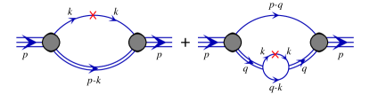
Figure 1: Feynman diagrams representing the quark distributions in the nucleon. The single line represents the quark propagator and the double line the diquark $t$-matrix. The shaded oval denotes the quark-diquark vertex function and the operator insertion has the form $\gamma^{+}\gamma_{5}\,\delta\!\left(x-\frac{k_{-}}{p_{-}}\right)\frac{1}{2}\left(1\pm\tau_{z}\right)$ for the spin-dependent distribution, while $\gamma^{+}\gamma_{5}\to\gamma^{+}$ for the spin-independent case.

III Results

The parameters for the quark-diquark model for the bound nucleon are discussed in Refs. Cloet:2005pp ; Cloet:2005rt , so we will not repeat them. The new features presented in this paper are those associated with finite nuclei. In Table 1 we give values for $\shortstack{\rule{8.63335pt}{0.6458pt}\\ [-0.5ex]$M$}_{N}$, $M_{N\kappa}$ and $V_{N\kappa}$ obtained from the single particle shell model. These values are then used in Eq. (11) to calculate the nuclear quark distributions.

The unpolarized EMC effect is defined as the ratio of the spin-averaged structure function, $F_{2A}$, of a particular nucleus $A$ divided by the naive expectation. That is

$$R_{A}=\frac{F_{2A}}{F_{2A}^{\text{naive}}}=\frac{F_{2A}}{Z\,F_{2p}+(A-Z)\,F_{2n}},$$ (22)

where $F_{2p}$ is the free proton structure function and $F_{2n}$ the free neutron structure function. In the limit of no Fermi motion and no medium effects of any kind, this ratio is unity. An equivalent EMC ratio can also be defined for the $K=0$ multipole.

The polarized EMC effect is defined by an analogous ratio, which is the spin-dependent structure function for a particular nucleus with helicity $H$, divided by the naive expectation, that is

$$R_{As}^{JH}=\frac{g_{1A}^{JH}}{g^{JH}_{1A,\text{naive}}}=\frac{g_{1A}^{JH}}{P^{JH}_{p}\,g_{1p}+P^{JH}_{n}\,g_{1n}}.$$ (23)

Here $g_{1p}$ and $g_{1n}$ are the free nucleon structure functions and $P^{JH}_{p(n)}$ is the polarization of the protons (neutrons) in the nucleus with helicity $H$, defined by

$$P^{JH}_{\alpha}=\langle J,H\lvert 2\,\hat{S}^{\alpha}_{z}\rvert J,H\rangle,\qquad\alpha\in\left(p,n\right),$$ (24)

where $\hat{S}_{z}^{\alpha}$ is the total spin operator for protons or neutrons. From an experimental standpoint one should simply use the best estimates of the polarization factors available in the literature. In this work we use the polarization factors obtained from the nonrelativistic limit of Eq. (24), which differ from the relativistic values calculated within our model by less than 2%. If only a single valence nucleon or nucleon-hole contributes to the nuclear polarization, then in the nonrelativistic limit the polarization factor is simply given by

$$P^{JH}_{\alpha}=\pm\frac{2\,H}{2\ell+1},$$ (25)

where $\ell$ is the orbital angular momentum and the $\pm$ refers to the cases $J=\ell\pm\tfrac{1}{2}$.

	$\shortstack{\rule{8.63335pt}{0.6458pt}\\ [-0.5ex]$M$}_{\!N}$	$M_{N\kappa}$				$V_{N\kappa}$
		-1	-2	1	-3	-1	-2	1	-3
7Li	933	811	856	–	–	89	58	–	–
11B	931	793	829	–	–	101	76	–	–
15N	929	785	815	815	–	106	86	86	–
27Al	930	771	794	793	820	115	101	101	82

Table 1: All quantities are in MeV. The labels $-$1, $-$2, 1, $-$3 refer to the Dirac quantum number $\kappa$, where $\lvert\kappa\rvert=j+\tfrac{1}{2}$.

The polarized EMC ratio can also be defined for the $K=1$ multipole structure function and has the form

$$R_{As}^{(J1)}=\frac{g_{1A}^{(J1)}}{P^{(J1)}_{p}\,g_{1p}+P^{(J1)}_{n}\,g_{1n}},$$ (26)

where $P^{(J1)}_{\alpha}$ is the reduced matrix element

$$P^{(J1)}_{\alpha}=\langle J\lvert\lvert\,2\,\hat{S}^{\alpha}\,\rvert\rvert J\rangle=\sqrt{\frac{(2J+1)(2J+2)}{6J}}\,P_{\alpha}^{JJ}.$$ (27)

Because the spin structure function $g_{1n}$ is smaller than $g_{1p}$ and remains poorly known, especially at large $x$, it is clear from Eqs. (23,26) that to determine the polarized EMC effect it is necessary to choose nuclei where $\lvert P_{n}\rvert\ll\lvert P_{p}\rvert$. There is also an upper limit on the mass number of nuclei that can be readily used to measure the polarized EMC effect, because for spin cross-sections the valence nucleons dominate and hence $g_{1A}$ is suppressed by approximately $1/A$ relative to $F_{2A}$, where all nucleons contribute.

The best candidates are nuclei with a single valence proton or proton-hole, for example the stable nuclei ¹¹B, ¹⁵N and ²⁷Al. Another good choice is ⁷Li, where the nuclear polarization is largely dominated by the valence proton. Extensive studies of ⁷Li, beginning in the 60’s with the shell model Cohen:1965qa , to modern state of the art Quantum Monte Carlo calculations Pudliner:1997ck , consistently find $P_{p}\simeq 0.86-0.88$. The Quantum Monte Carlo result for the neutron polarization is $P_{n}\simeq-0.04$.

First we discuss the nuclear quark distributions, focusing on ⁷Li as its treatment is a little more involved compared with the other nuclei, because there are three valence nucleons coupled to $J=3/2$ and $T=1/2$. Using the $H=3/2$ shell model wavefunction found in Refs. Landau:1977 ; Guzey:1999rq , when evaluating the spin-independent analogue of Eq. (11) for the $u$-quark distribution in ⁷Li we obtain

$$u_{A}^{3/2\,3/2}(x_{A})=2\left[u_{p,-1}^{1/2}(x_{A})+d_{p,-1}^{1/2}(x_{A})\right]\\ +\frac{1}{15}\biggl{[}13\,u_{p,-2}^{3/2}(x_{A})+20\,d_{p,-2}^{3/2}(x_{A})\\ +2u_{p,-2}^{1/2}(x_{A})+10\,d_{p,-2}^{1/2}(x_{A})\biggr{]},$$ (28)

where we have used charge symmetry to relate $u_{n}\leftrightarrow d_{p}$. The spin-dependent distribution has the form

$$\Delta u_{A}^{\,3/2\,3/2}(x_{A}) =\frac{1}{15}\left[13\,\Delta u_{p,-2}^{3/2}(x_{A})+2\,\Delta d_{p,-2}^{3/2}(x_{A})\right].$$ (29)

Similar expressions hold for the $H=1/2$ and $d$-quark distributions. With this wavefunction the ⁷Li polarization factors are $P_{p}^{JH}=\tfrac{2H}{3}\tfrac{13}{15}$ and $P_{n}^{JH}=\tfrac{2H}{3}\tfrac{2}{15}$. For the other nuclei the situation is simpler as we make the approximation that the nuclear spin is carried solely by the valence proton-hole.

In Figs. 3-5 we show the leading multipole quark distributions for ¹¹B, together with the next-to-leading $K=3$ multipole for the spin-dependent case, at the model scale of $Q_{0}^{2}=0.16~{}$GeV² Cloet:2005pp . The other nuclear quark distributions are similar, so we will not show them. The dotted line is the result without Fermi motion and medium effects, and is obtained from expressions like Eq. (11) by replacing each smearing function with a delta function (multiplied by the polarization factor for the spin-dependent case) and using the free results for the $u$- and $d$-quark distributions in the nucleon. The dot-dashed line includes the effect of the scalar field, and the dashed curve also incorporates Fermi motion, which is the result after convolution with the appropriate nucleon distribution (Eqs. (14,15)). The complete in-medium distribution is given by the solid line and is the result obtained after also shifting the scaling variable using Eq. (21).

For the spin-independent distributions all nucleons contribute. Therefore, in Figs. 3 and 3 we see that the $u$- and $d$-quark distributions are very similar. For the spin-dependent case (see Fig. 5) only the valence proton-hole contributes. Hence the distributions resemble those of the proton. We find that higher multipole distributions are greatly suppressed relative to the leading results, see for example the $K=3$ distribution in Fig. 5. The spin-independent $K=2$ multipole is an order of magnitude smaller again and reflects the very weak helicity dependence of the $F_{2A}^{JH}$ structure functions. This weak helicity dependence arises because the spin-zero core is the dominant contribution to $F_{2A}^{JH}$, and changes in $H$ simply reflect different spin orientations of the valence nucleon(s).

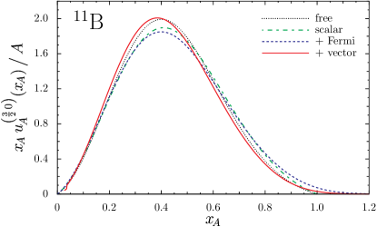
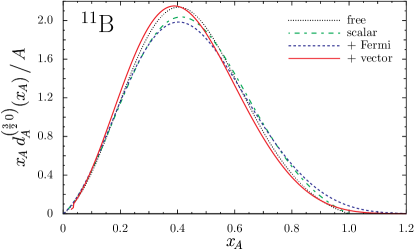
Figure 2: The first spin-independent multipole (K=0) $u$-quark distribution in ¹¹B (at $Q^{2}=Q_{0}^{2}$).

Figure 3: The first spin-independent multipole (K=0) $d$-quark distribution in ¹¹B (at $Q^{2}=Q_{0}^{2}$).

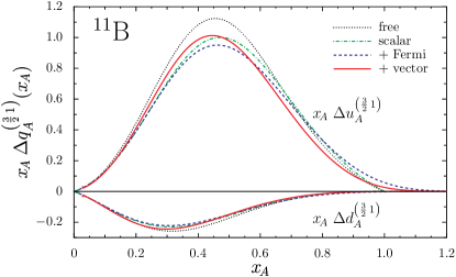
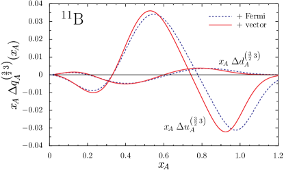
Figure 4: The first spin-dependent multipole (K=1) $u$- and $d$-quark distributions in ¹¹B (at $Q^{2}=Q_{0}^{2}$).

Figure 5: The second spin-dependent multipole (K=3) $u$- and $d$-quark distributions in ¹¹B (at $Q^{2}=Q_{0}^{2}$).

The main features of the medium effects displayed in Figs. 3 – 5 are similar to those found in our earlier nuclear matter calculation Cloet:2005rt . The spin-independent distributions are quenched at large $x$ and enhanced for small $x$, whereas the spin-dependent distributions are quenched for all $x$.

The nuclear spin sum, $\Sigma^{(A)}$, and axial coupling, $g_{A}^{(A)}$, contain information on both nuclear and quark effects and are simply given by

$$\Sigma^{(A)} =\Delta u_{A}+\Delta d_{A}\equiv\Sigma\,\left(P_{p}+P_{n}\right),$$ (30)

$$g_{A}^{(A)} =\Delta u_{A}-\Delta d_{A}\equiv g_{A}\,\left(P_{p}-P_{n}\right),$$ (31)

where $\Delta q_{A}$ represents the first moment of $\Delta q_{A}^{JJ}$ and $\Sigma$, $g_{A}$ are the medium modified nucleon quantities, defined by dividing out the non-relativistic isoscalar and isovector polarization factors for $H=J$. We find that $\Sigma$ and $g_{A}$ are both suppressed in-medium relative to the free values, as summarized Table 2. This decrease of $g_{A}$ in-medium is in agreement with the well known nuclear $\beta$-decay studies which, after taking into account the nuclear structure effects, require a quenching of $g_{A}$ to achieve agreement with empirical data.

	$\Delta u$	$\Delta d$	$\Sigma$	$g_{A}$
$p$	0.97	-0.30	0.67	1.267
7Li	0.91	-0.29	0.62	1.19
11B	0.88	-0.28	0.60	1.16
15N	0.87	-0.28	0.59	1.15
27Al	0.87	-0.28	0.59	1.15
Nucl. Matter	0.74	-0.25	0.49	0.99

Table 2: Results for the first moment of the in-medium quark distributions in the bound proton and the resulting spin sum and nucleon axial charge. It is clear that the moments tend to decrease with increasing $A$.

In Figs. 7 – 9 we give results for the EMC and polarized EMC effect in ⁷Li, ¹¹B, ¹⁵N and ²⁷Al at $Q^{2}=5\,$GeV². The dashed line is the unpolarized EMC effect, the solid line is the $K=1$ polarized EMC effect and the dotted line is the $M=J$ polarized EMC result (c.f. Eqs. (26) and (23), respectively). For the unpolarized EMC effect the results agree very well with the experimental data taken from Ref. Gomez:1993ri , where importantly we obtain the correct $A$-dependence.

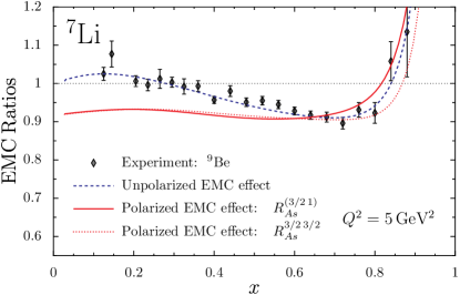
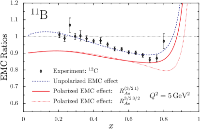
Figure 6: The EMC and polarized EMC effect in ⁷Li. The empirical data is from Ref. Gomez:1993ri .

Figure 7: The EMC and polarized EMC effect in ¹¹B. The empirical data is from Ref. Gomez:1993ri .

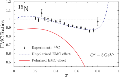
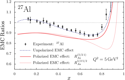
Figure 8: The EMC and polarized EMC effect in ¹⁵N. The empirical data is from Ref. Gomez:1993ri .

Figure 9: The EMC and polarized EMC effect in ²⁷Al. The empirical data is from Ref. Gomez:1993ri .

Consistent with previous nuclear matter studies, we find that the polarized EMC effect is larger than the unpolarized case, with the exception of the multipole result for ⁷Li at $x\gtrsim 0.6$. Based on the wavefunction in Ref. Guzey:1999rq the neutrons give a small contribution to the polarization. To test the dependence on the neutron polarization we also coupled the two neutrons to spin-zero, so that $P_{n}^{3/2\,3/2}=0$, which is closer to the Quantum Monte Carlo result of $-0.04\,$Pudliner:1997ck . We find that these results are very similar to those in Fig. 7.

The unusual shape for the ¹⁵N polarized EMC result is because our full result for $g_{1A}^{1/2\,1/2}$ changes sign at $x\simeq 0.8$, and hence the ratio must go to zero at this point. The origin of this sign change is the nucleon $p_{1/2}$ smearing function, which becomes positive for large $y_{A}$. This result suggests ¹⁵N may not be a good candidate with which to study nucleon medium modifications. The ¹¹B and ²⁷Al results resemble those obtained for nuclear matter Cloet:2005rt , where we find a polarized EMC effect roughly twice that of the unpolarized case.

IV Conclusion

Using a relativistic formalism, where the quarks in the bound nucleons respond to the nuclear environment, we calculated the quark distributions and structure functions of ⁷Li, ¹¹B, ¹⁵N and ²⁷Al. For a spin-$J$ target there are $2J+1$ independent quark distributions or structure functions in the Bjorken limit. For example, ²⁷Al therefore has six structure functions, however we find that the higher multipoles are suppressed relative to the leading result by at least an order of magnitude.

We were readily able to describe the EMC effect in these nuclei, and importantly obtained the correct $A$-dependence. Although we do not show the results, we also determined the EMC ratio for ¹²C, ¹⁶O and ²⁸Si and found results very similar to their $A-1$ neighbours. In Eq. (23) we define the polarized EMC ratio in nuclei. This ratio is such that in the extreme nonrelativistic limit, with no medium modifications, it is unity. The results for the polarized EMC effect in nuclei corroborate earlier nuclear matter Cloet:2005rt ; Smith:2005ra , light nuclei Steffens:1998rw and small $x$ Guzey:1999rq studies that found large medium modifications to the spin structure function relative to the unpolarized case. In particular, we find that the fraction of the spin of the nucleon carried by the quarks is decreased in nuclei (see Table 2). If this result is confirmed experimentally, it would give important insights into in-medium quark dynamics and help quantify the role of quark degrees of freedom in the nuclear environment.

References

- (1) P. A. M. Guichon, Phys. Lett. B 200, 235 (1988).
- (2) K. Saito and A. W. Thomas, Phys. Rev. C 52, 2789 (1995) [arXiv:nucl-th/9506003].
- (3) P. A. M. Guichon, K. Saito, E. N. Rodionov and A. W. Thomas, Nucl. Phys. A 601, 349 (1996) [arXiv:nucl-th/9509034].
- (4) P. A. M. Guichon and A. W. Thomas, Phys. Rev. Lett. 93, 132502 (2004) [arXiv:nucl-th/0402064].
- (5) P. A. M. Guichon, H. H. Matevosyan, N. Sandulescu and A. W. Thomas, arXiv:nucl-th/0603044.
- (6) M. Arneodo, Phys. Rept. 240, 301 (1994).
- (7) D. F. Geesaman, K. Saito and A. W. Thomas, Ann. Rev. Nucl. Part. Sci. 45, 337 (1995).
- (8) J. J. Aubert et al. [European Muon Collaboration], Phys. Lett. B 123, 275 (1983).
- (9) G. A. Miller and J. R. Smith, Phys. Rev. C 65, 015211 (2002) [Erratum-ibid. C 66, 049903 (2002)] [arXiv:nucl-th/0107026].
- (10) G. Piller and W. Weise, Phys. Rept. 330, 1 (2000) [arXiv:hep-ph/9908230].
- (11) I. C. Cloët, W. Bentz and A. W. Thomas, Phys. Rev. Lett. 95, 052302 (2005) [arXiv:nucl-th/0504019].
- (12) A. Arima, K. Shimizu, W. Bentz and H. Hyuga, Adv. Nucl. Phys. 18, 1 (1987).
- (13) J. Morgenstern and Z. E. Meziani, Phys. Lett. B 515, 269 (2001) [arXiv:nucl-ex/0105016].
- (14) A. Aste, C. von Arx and D. Trautmann, Eur. Phys. J. A 26, 167 (2005) [arXiv:nucl-th/0502074].
- (15) S. Strauch et al. [Jefferson Lab E93-049 Collaboration], Phys. Rev. Lett. 91, 052301 (2003) [arXiv:nucl-ex/0211022].
- (16) S. Dieterich et al., Phys. Lett. B 500, 47 (2001) [arXiv:nucl-ex/0011008].
- (17) J. M. Udias and J. R. Vignote, Phys. Rev. C 62, 034302 (2000) [arXiv:nucl-th/0007047].
- (18) D. H. Lu, A. W. Thomas, K. Tsushima, A. G. Williams and K. Saito, Phys. Lett. B 417, 217 (1998) [arXiv:nucl-th/9706043].
- (19) R. L. Jaffe, MIT-CTP-1261 Lectures presented at the Los Alamos School on Quark Nuclear Physics, Los Alamos, N.Mex., Jun 10-14, 1985.
- (20) P. Hoodbhoy, R. L. Jaffe and A. Manohar, Nucl. Phys. B 312, 571 (1989).
- (21) R. L. Jaffe and A. Manohar, Nucl. Phys. B 321, 343 (1989).
- (22) H. Mineo, W. Bentz, N. Ishii, A. W. Thomas and K. Yazaki, Nucl. Phys. A 735, 482 (2004) [arXiv:nucl-th/0312097].
- (23) I. C. Cloët, W. Bentz and A. W. Thomas, Phys. Lett. B 621, 246 (2005) [arXiv:hep-ph/0504229].
- (24) A. Buck, R. Alkofer and H. Reinhardt, Phys. Lett. B 286, 29 (1992).
- (25) S. Cohen and D. Kurath, Nucl. Phys. 73, 1 (1965).
- (26) B. S. Pudliner, V. R. Pandharipande, J. Carlson, S. C. Pieper and R. B. Wiringa, Phys. Rev. C 56, 1720 (1997) [arXiv:nucl-th/9705009].
- (27) L. D. Landau and E. M. Lifshitz, Quantum Mechanics, Non-relativistic Theory (Pergamon, New York, 1977).
- (28) V. Guzey and M. Strikman, Phys. Rev. C 61, 014002 (2000) [arXiv:hep-ph/9903508].
- (29) B. A. Brown and B. H. Wildental, Phys. Rev. C 28, 2397 (1983).
- (30) T. Suzuki, R. Fujimoto and T. Otsuka, Phys. Rev. C 67, 044302 (2003).
- (31) J. Gomez et al., Phys. Rev. D 49, 4348 (1994).
- (32) J. R. Smith and G. A. Miller, Phys. Rev. C 72, 022203 (2005) [arXiv:nucl-th/0505048].
- (33) F. M. Steffens, K. Tsushima, A. W. Thomas and K. Saito, Phys. Lett. B 447, 233 (1999) [arXiv:nucl-th/9810018].
- (34) M. Miyama and S. Kumano, Comput. Phys. Commun. 94, 185 (1996) [arXiv:hep-ph/9508246].
- (35) M. Hirai, S. Kumano and M. Miyama, Comput. Phys. Commun. 108, 38 (1998) [arXiv:hep-ph/9707220].