Gauge-invariant approach to meson photoproduction
including the final-state interaction

H. Haberzettl Center for Nuclear Studies, Department of Physics, The George Washington University, Washington, DC 20052, USA Institut für Kernphysik (Theorie), Forschungszentrum Jülich, D-52425 Jülich, Germany    K. Nakayama Department of Physics and Astronomy, University of Georgia, Athens, GA 30602, USA Institut für Kernphysik (Theorie), Forschungszentrum Jülich, D-52425 Jülich, Germany    S. Krewald Institut für Kernphysik (Theorie), Forschungszentrum Jülich, D-52425 Jülich, Germany
(23 May 2006)
Abstract

A fully gauge-invariant (pseudoscalar) meson photoproduction amplitude off a nucleon including the final-state interaction is derived. The approach based on a comprehensive field-theoretical formalism developed earlier by one of the authors replaces certain dynamical features of the full interaction current by phenomenological auxiliary contact currents. A procedure is outlined that allows for a systematic improvement of this approximation. The feasibility of the approach is illustrated by applying it to both the neutral and charged pion photoproductions.

pacs:
25.20.Lj, 13.60.Le, 24.10.Jv

I Introduction

Ever since the pioneering work by Chew, Goldberger, Low, and Nambu on pion production Chew , the study of photo- and electroproduction of mesons off nucleons has been utilized as one of the major research avenues to learn about the excited states of the nucleon. In order to extract accurate information on nucleon resonances, one needs — in addition to precise and extensive experimental data — reliable reaction theories that allow one to disentangle the resonance contributions from the background contributions to the observables.

The extant descriptions of meson photoproduction reactions span a wide range of different approaches (e.g., Chiral Perturbation Theory, tree-level effective Lagrangians, $K$-matrix approach, etc. BKLM ; Bernard:1991rt ; Bernard:1992nc ; Bernard ; Feuster ; Penner ; Scholten ; DHKT ; Hanstein ). The present work is based on the dynamical framework of meson-exchange models of hadronic interactions Nozawa ; Surya ; Sato ; Pascalutsa in which the composite nature of hadronic vertices is accounted for by so-called form factors. Since, at present, our theoretical understanding of these vertex form factors is rather incomplete, one usually parameterizes the vertex structure by phenomenological functions (usually of monopole or dipole form) whose parameters are adjusted to fit the data. The presence of such form factors spoils gauge invariance of the photoproduction amplitude already when dressing the bare tree level in this phenomenological manner. The inclusion of an explicit hadronic final-state interaction (FSI) further complicates this problem since the construction of the corresponding interaction current (where the photon interacts with the hadronic structure within the vertex) consistent with the FSI requires the knowledge of the underlying dynamical structure, a requirement that is impossible to be satisfied in an approach where phenomenological form factors are employed. In order to maintain gauge invariance in this situation, one needs to resort to finding prescriptions that are consistent at a phenomenological level with the various dynamical models. The existing prescriptions Gross ; Ohta ; Antw ; HH1 ; HH2 ; Kvinikhidze ; DW ; Borasoy:2005zg do not, and indeed cannot, provide a unique answer to this problem since manifestly transverse currents — that have no bearing on gauge invariance — can always be added to any given prescription. From a phenomenological point of view, therefore, it is unavoidable that one seeks a prescription that works best in reproducing the data (see, e.g., discussion in Usov ). A number of the existing gauge-invariance preserving prescriptions have already been applied in this manner in pion photoproduction Surya ; Sato ; Pascalutsa as well as in electroproduction Nozawa1 ; Caia reactions.

However, most of the existing calculations based on phenomenological dynamical models are actually not gauge invariant. In fact, they revert to a variety of ad hoc recipes for the sole purpose of enforcing current conservation,

$$k_{\mu}M^{\mu}=0~{},$$ (1)

when the production current $M^{\mu}$ is on-shell, but not the gauge-invariance condition expressed by the generalized Ward–Takahashi (WT) identity kazes ; Antw ; HH1

$\displaystyle k_{\mu}M^{\mu}$ $\displaystyle=-|F_{s}\tau\rangle S_{p+k}Q_{i}S^{-1}_{p}+S^{-1}_{p^{\prime}}Q_{f}S_{p^{\prime}-k}|F_{u}\tau\rangle$
$\displaystyle\qquad\mbox{}+\Delta^{-1}_{p-p^{\prime}+k}Q_{\pi}\Delta_{p-p^{\prime}}|F_{t}\tau\rangle~{},$ (2)

which is an off-shell condition. [This equation is repeated as Eq. (8) below, where its details are explained.]

One of the few exceptions to this situation is the recent work by Pascalutsa and Tjon Pascalutsa where a fully gauge invariant pion photoproduction amplitude has been constructed based on the Gross–Riska prescription Gross . This approach has been extended and applied as well to pion electroproduction Caia . The prescription of Ref. Gross also has been applied to the nucleon-nucleon bremsstrahlung reaction Fred . The Gross–Riska procedure relies on the observation that vertices and propagators always enter in the combination (vertex $\times$ propagator) in a given reaction amplitude. Therefore, a vertex form factor that depends only on the momentum of the propagating (off-shell) particle can be incorporated into the corresponding propagator instead of being associated with the vertex. Of course, if more than one leg of the vertex belongs to an off-shell particle, this restricts the phenomenological form factors to being separable functions of the respective leg momenta. In addition, the form factors should be such that they do not lead to unphysical behavior of the resulting propagators. Gauge invariance is then fulfilled by constructing electromagnetic currents that obey the WT identities with the respective hadronic propagators modified by the inclusion of the form factors as described.111Note that the electromagnetic vertices constructed in this way in Refs.Pascalutsa ; Fred differ from each other by a transverse piece. At the tree level, this prescription completely removes the form factors from the longitudinal part of the reaction amplitude; i.e., only manifestly transverse parts of the production current carry any form factor dependence.

In the present work, we construct a photoproduction amplitude based on the field-theoretical approach given by Haberzettl HH1 . The full formalism is gauge-invariant as a matter of course. However, in view of its complexity and high nonlinearity, its practical implementations require that some reaction mechanisms need to be truncated and/or replaced by phenomenological approximations. Our objective here is to preserve full gauge invariance, in the sense of Eq. (2), for this approximate treatment, but allowing for the presence of explicit hadronic FSIs. This problem has been treated already in Ref. HH3 as a two-step procedure where the gauge-invariant treatment of explicit FSIs was added on to an already gauge-invariant tree-level amplitude that had been constructed according to the prescriptions given in Ref. HH2 . The present approach instead starts from the full amplitude and derives a single condition for the mechanisms to be approximated that follows directly from the generalized WT identity (2). It thus is more general and not tied to any particular tree-level treatment. Moreover, we present a general scheme that allows a systematic way of including more complex reaction mechanisms into the procedure. At the lowest order, it is found that the essential aspects of the results found in Ref. HH3 remain true. In contrast to the prescription of Ref. Gross , the present approach does not impose any restriction on the type of the hadronic form factors that can be used. Furthermore, the longitudinal part of the resulting reaction amplitude retains these form factors even at the tree-level.

The present paper is organized as follows. In Sec. II we present our approach to construct a fully gauge invariant photoproduction amplitude. In Sec. III we illustrate the approach developed in sect. II by applying it to the pion photoproduction. Section IV contains a summary with our conclusions. Some details of the present approach as well as of its model application are given in the appendices.

Refer to caption
Figure 1: (Color online) Diagrammatic summary of the field-theory formalism of Ref. HH1 . Time proceeds from right to left.   (a)  Meson production current $M^{\mu}$. The first line corresponds to Eq. (3) summing up, in that order, the $s$-, $u$-, and $t$-channel diagrams and the interaction current $M^{\mu}_{\rm int}$. (The different colors of the hadronic three-point vertices identify the $\pi NN$ vertex in different kinematical situations.) The dynamical content of $M^{\mu}_{\rm int}$ is explicitly shown by the diagrams enclosed in the dashed box of the last two lines. This also includes, in the bottom line, the final-state interaction mediated by the nonpolar $\pi N$ amplitude $X$ that satisfies the integral equation shown in (b). The diagram element labeled $U$ subsumes all exchange currents $U^{\mu}$ contributing to the process (see Fig. 2). The diagram with open circle depicts the bare current $m^{\mu}_{\rm bare}$ (i.e., the Kroll–Ruderman term).   (b)  Pion-nucleon scattering with dressed hadrons. The full $\pi N$-amplitude is denoted by $T$, with $X$ subsuming all of its nonpolar (i.e., non-$s$-channel) contributions. The latter satisfies the integral equation $X=U+UG_{0}X$ depicted in the third line here, where the driving term $U$ sums up all nonpolar irreducible contributions to $\pi N$-scattering, i.e., all irreducible contributions which do not contain an $s$-channel pole (see Ref. HH1 for full details). — In both parts (a) and (b), diagram elements with open, unlabeled circles describe bare quantities, and solid circles (or circles filled with colors) denote the corresponding dressed vertices and propagators.

II Formalism

In the following, for definiteness, we will explicitly consider the production of pions off the nucleon, i.e., $\gamma+N\to\pi+N$, but the formalism will of course apply equally well to the photoproduction (or electroproduction) of any pseudoscalar meson. Moreover, at intermediate stages of the reaction, we will ignore other mesons or baryonic states since they are irrelevant for the problem at hand, namely how to preserve gauge invariance in the presence of FSI.

Refer to caption
Figure 2: (Color online) Exchange-current contributions subsumed in $U^{\mu}$ grouped by the topological properties of the underlying $\pi N$ irreducible hadron contributions: The diagrams subsumed in $E^{\mu}$ are based on the photon attaching itself internally in all possible ways to a simple hadron exchange graph, whereas $D^{\mu}$ subsumes the analogous contributions arising from a triangular hadron graph; more complex structures are not shown explicitly. Note that the second and third diagrams of $E^{\mu}$, and the first and third diagrams of $D^{\mu}$ explicitly contain the full off-shell interaction current $M^{\mu}_{\text{int}}$. Implicitly it is contained in many more places. (The middle diagram in the second row of $D^{\mu}$ contains the diagram $X^{\mu}$ where the photon is attached to the internal structure of the non-polar $\pi N$ amplitude $X$. The details of this mechanism are irrelevant for the present considerations; they can be found in Ref. HH1 .)

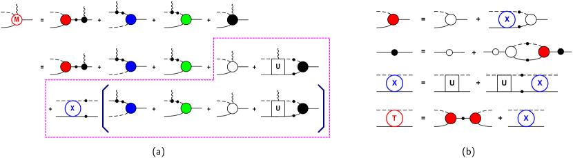
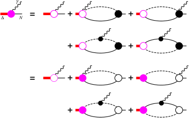
As mentioned, our approach is based on the field-theory formalism of Ref. HH1 . For the present purpose, however, we do not need to recapitulate its full details. Instead, we employ the summarizing diagrams of Figs. 1, 2, and 3. As is well-known Chew , the photoproduction current $M^{\mu}$ can be broken down according to

$$M^{\mu}=M^{\mu}_{s}+M^{\mu}_{u}+M^{\mu}_{t}+M^{\mu}_{\text{int}}~{},$$ (3)

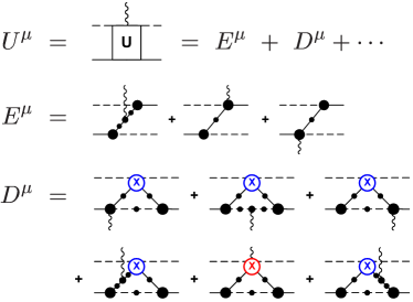
where the first three terms describe the coupling of the photon to external legs of the underlying $\pi NN$ vertex (with subscripts $s$, $u$, and $t$ referring to the appropriate Mandelstam variables of their respective intermediate hadrons). These terms are relatively straightforward and easy to implement in a practical application. However, the last term, the interaction current $M^{\mu}_{\text{int}}$, where the photon couples inside the vertex, explicitly contains the hadronic FSI; its structure is, therefore, more complex than that of any of the first three terms. We read off the diagrams enclosed by the dashed box of Fig. 1(a) that

$\displaystyle M^{\mu}_{\text{int}}$ $\displaystyle=m^{\mu}_{\text{bare}}+U^{\mu}G_{0}|F\tau\rangle$
$\displaystyle\quad\mbox{}+XG_{0}\Big{(}M^{\mu}_{u}+M^{\mu}_{t}+m^{\mu}_{\text{bare}}+U^{\mu}G_{0}|F\tau\rangle\Big{)}~{},$ (4)

where $m^{\mu}_{\text{bare}}$ is the bare Kroll–Ruderman contact current, $U^{\mu}$ subsumes all possible exchange currents (see Fig. 2), $G_{0}$ describes the intermediate $\pi N$ two-particle propagation, and the FSI is mediated by the nonpolar part $X$ of the $\pi N$ $T$ matrix. Following Ref. HH1 , the notation $|F\tau\rangle$ is used for the dressed $N\to\pi N$ vertex (including its full coupling-operator structure); for $N\pi\to N$ with the pion leg reversed, we use $\langle F\tau|$. The isospin operator $\tau$ (with its component index suppressed) is pulled out of the vertex explicitly for later convenience [see Eq. (12)]. The vertex obeys the equation

$$|F\tau\rangle=\left(1+XG_{0}\right)|F_{\text{bare}}\tau\rangle\ ,$$ (5)

where $|F_{\text{bare}}\tau\rangle$ denotes the bare $\pi NN$ vertex.

Refer to caption
Figure 3: Diagrammatic representation of the nucleon’s electromagnetic current obtained by attaching a photon to the second line of diagrams in Fig. 1(b). The terms correspond to those of Eq. (6).

Note that the $NN\gamma$ electromagnetic vertices appearing in Fig. 1(a), are also fully dressed vertices given by

$\displaystyle\Gamma^{\mu}_{N}$ $\displaystyle={\Gamma^{\mu}_{N}}_{\text{bare}}+\bar{m}^{\mu}_{\text{bare}}G_{0}|F\tau\rangle$
$\displaystyle\quad\mbox{}+\langle F\tau|G_{0}\Big{(}m^{\mu}_{\text{bare}}+M^{\mu}_{t}+M^{\mu}_{u}+U^{\mu}G_{0}|F\tau\rangle\Big{)}~{},$ (6)

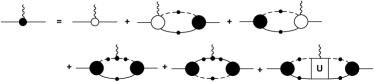
and illustrated diagrammatically in Fig. 3. ${\Gamma^{\mu}_{N}}_{\text{bare}}$ and $\bar{m}^{\mu}_{\text{bare}}$ denote the bare vertices for $\gamma N\to N$ and $\gamma\pi N\to N$ (i.e., $\bar{m}^{\mu}_{\text{bare}}$ is the Kroll–Ruderman current $m^{\mu}_{\text{bare}}$ with the pion leg reversed). Also, the nucleon propagator, $S$, illustrated in the second row from the top in Fig. 1(b), is fully dressed according to

$$S^{-1}=S^{-1}_{\text{bare}}-\langle F_{\text{bare}}\tau|G_{0}|F\tau\rangle\ ,$$ (7)

such that the WT identity as expressed by Eq. (10a) below is satisfied. $S_{\text{bare}}$ stands for the bare nucleon propagator.

As alluded to in the Introduction, the production current $M^{\mu}$ is gauge invariant if its four-divergence satisfies the generalized WT identity HH1 ; kazes ; Antw

$\displaystyle k_{\mu}M^{\mu}$ $\displaystyle=-|F_{s}\tau\rangle S_{p+k}Q_{i}S^{-1}_{p}+S^{-1}_{p^{\prime}}Q_{f}S_{p^{\prime}-k}|F_{u}\tau\rangle$
$\displaystyle\qquad\mbox{}+\Delta^{-1}_{p-p^{\prime}+k}Q_{\pi}\Delta_{p-p^{\prime}}|F_{t}\tau\rangle~{},$ (8)

where $p$ and $k$ are the four-momenta of the incoming nucleon and photon, respectively, and $p^{\prime}$ and $q$ are the four-momenta of the outgoing nucleon and pion, respectively, related by momentum conservation $p^{\prime}+q=p+k$. $S$ and $\Delta$ are the propagators of the nucleons and pions, respectively, with their subscripts denoting the available four-momentum for the corresponding hadron; $Q_{i}$, $Q_{f}$, and $Q_{\pi}$ are the initial and final nucleon and the pion charge operators, respectively. The index $x$ at $[F_{x}\tau]$ labels the appropriate kinematic situation for $\pi NN$ vertex in the $s$-, $u$-, or $t$-channel diagrams of Fig. 1. This is an off-shell condition. In view of the inverse propagators appearing in each term here, if all external hadronic legs are on-shell, this reduces to

$$k_{\mu}M^{\mu}=0\qquad\text{(hadrons on-shell)}~{},$$ (9)

which describes current conservation.

Physically relevant, of course, is only current conservation. However, the reason one must satisfy the off-shell condition (8) for gauge invariance to hold true is the requirement to have consistency across all elements of the underlying reaction dynamics. In view of the inherent nonlinearity of the process (due to the fact that the number of pions is not conserved), the elements contributing to the full amplitude $M^{\mu}$ couple back into themselves nonlinearly HH1 : For example, as can be seen from Fig. 2, the sum of exchange currents $U^{\mu}$ internally also contains the interaction current $M^{\mu}_{\text{int}}$ in several places, with at least one hadron leg off-shell even if all external hadrons are taken on-shell. It is then found that it is not possible to achieve current conservation consistently unless the current satisfies the off-shell condition (8), which translates into the condition (11) for the interaction current given below.

The electromagnetic currents for the nucleons and the pions, $\Gamma^{\mu}_{N}$ and $\Gamma^{\mu}_{\pi}$, respectively, satisfy the WT identities

$\displaystyle k_{\mu}\Gamma_{N}^{\mu}(p^{\prime},p)$ $\displaystyle=S^{-1}_{p^{\prime}}Q_{N}-Q_{N}S^{-1}_{p}~{},$ (10a)
$\displaystyle k_{\mu}\Gamma_{\pi}^{\mu}(q^{\prime},q)$ $\displaystyle=\Delta^{-1}_{q^{\prime}}Q_{\pi}-Q_{\pi}\Delta^{-1}_{q}~{},$ (10b)

where the four-momentum relations $p^{\prime}=p+k$ and $q^{\prime}=q+k$ hold. It is therefore possible to replace the generalized WT identity (8) by the equivalent gauge-invariance condition

$\displaystyle k_{\mu}M^{\mu}_{\text{int}}$ $\displaystyle=-|F_{s}\tau\rangle Q_{i}+Q_{f}|F_{u}\tau\rangle e_{f}+Q_{\pi}|F_{t}\tau\rangle$
$\displaystyle\equiv-|F_{s}\rangle e_{i}+|F_{u}\rangle e_{f}+|F_{t}\rangle e_{\pi}~{},$ (11)

where the operators

$$e_{i}=\tau Q_{i}~{},\quad e_{f}=Q_{f}\tau~{},\quad\text{and}\quad e_{\pi}=Q_{\pi}\tau$$ (12)

describe the respective hadronic charges in an appropriate isospin basis (component indices and summations are suppressed here), i.e, apart from some numerical factors, the $e_{x}$ are essentially given by the charges of the respective particles. Charge conservation for the production process then simply reads

$$e_{i}=e_{f}+e_{\pi}~{}.$$ (13)

In the following, it is more convenient to use the condition (11), instead of (8), together with (10).

We emphasize here that if the single-particle electromagnetic currents satisfy the WT identities (10) and if the four-divergence of the interaction current is given by (11), then the corresponding production amplitude $M^{\mu}$ will be gauge-invariant as a matter of course even if propagators and vertices have been subjected to approximations.

II.1 Preserving gauge invariance

Refer to caption
Figure 4: Diagrammatic representation of Eq. (14).

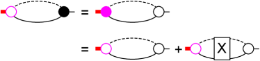
The preceding considerations are completely general. In practical applications, however, one will not be able to calculate all mechanisms that contribute to the full reaction dynamics and one must make some approximations. This is particularly true for the complex mechanisms that enter $U^{\mu}$, as depicted in Fig. 2. Approximations should preserve the gauge invariance of the amplitude. To see how this can be done, let us define
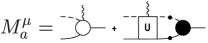
$$M^{\mu}_{a}=m^{\mu}_{\text{bare}}+U^{\mu}G_{0}|F\tau\rangle~{},$$ (14)

which is shown in Fig. 4, and thus write

$$M^{\mu}_{\text{int}}=M^{\mu}_{a}+XG_{0}\Big{(}M^{\mu}_{u}+M^{\mu}_{t}+M^{\mu}_{a}\Big{)}~{},$$ (15)

and recast the gauge-invariance condition (11) as a condition for $M^{\mu}_{a}$. This immediately produces

$\displaystyle k_{\mu}M^{\mu}_{a}$ $\displaystyle=(1-UG_{0})\big{[}-|F_{s}\rangle e_{i}+|F_{u}\rangle e_{f}+|F_{t}\rangle e_{\pi}\big{]}$
$\displaystyle\mbox{}\qquad-UG_{0}\big{[}k_{\mu}(M^{\mu}_{u}+M^{\mu}_{t})\big{]}~{},$ (16)

where

$$(1+XG_{0})^{-1}=1-UG_{0}$$ (17)

and

$$U=\left(1+XG_{0}\right)^{-1}X$$ (18)

were used, with $U$ being the sum of all non-polar hadronic driving terms [cf. third line of diagrams in Fig. 1(b)]. In the last term of (16) obviously only the non-transverse parts of the $u$- and $t$-channel currents $M^{\mu}_{u}$ and $M^{\mu}_{t}$ will contribute. Denoting those respectively by $m^{\mu}_{u}$ and $m^{\mu}_{t}$, i.e.,

$$k_{\mu}(M^{\mu}_{u}-m^{\mu}_{u})=0\quad\text{and}\quad k_{\mu}(M^{\mu}_{t}-m^{\mu}_{t})=0~{},$$ (19)

we finally have

$\displaystyle k_{\mu}M^{\mu}_{a}$ $\displaystyle=(1-UG_{0})\big{[}-|F_{s}\rangle e_{i}+|F_{u}\rangle e_{f}+|F_{t}\rangle e_{\pi}\big{]}$
$\displaystyle\mbox{}\qquad-k_{\mu}UG_{0}(m^{\mu}_{u}+m^{\mu}_{t})$ (20)

as the necessary condition that $M_{a}^{\mu}$ must satisfy so that $M^{\mu}_{\text{int}}$ yields the gauge-invariance condition (11). Equation (20) is exact — no approximation has been made up to here.

II.1.1 Approximating $M^{\mu}_{a}$

The structure of the preceding condition suggests the following approximation strategy. The condition evidently is satisfied if we now approximate $M^{\mu}_{a}$ by

$$M_{a}^{\mu}=(1-UG_{0})M^{\mu}_{c}-UG_{0}(m^{\mu}_{u}+m^{\mu}_{t})+T^{\mu}~{},$$ (21)

where $M^{\mu}_{c}$ can be any contact current satisfying

$$k_{\mu}M^{\mu}_{c}=-|F_{s}\rangle e_{i}+|F_{u}\rangle e_{f}+|F_{t}\rangle e_{\pi}$$ (22)

and $T^{\mu}$ is an undetermined transverse contact current that is unconstrained by the four-divergence (20). With the choice (21), the corresponding approximate $M^{\mu}_{\text{int}}$ is then easily found from (15) as

$\displaystyle M^{\mu}_{\text{int}}$ $\displaystyle=M_{c}^{\mu}+T^{\mu}$
$\displaystyle\mbox{}\quad+XG_{0}\big{[}(M^{\mu}_{u}-m^{\mu}_{u})+(M^{\mu}_{t}-m^{\mu}_{t})+T^{\mu}\big{]}~{}.$ (23)

In this scheme, therefore, the choice one makes for $M^{\mu}_{c}$ (and $T^{\mu}$) corresponds to an implicit approximation of the full dynamics contained in the right-hand side of Eq. (14). Moreover, beyond this actual choice, the only explicit effect of the FSI $X$ is from explicitly transverse loop contributions, which is precisely the same result that was found in Ref. HH3 . Thus it follows that

$$k_{\mu}M^{\mu}_{\text{int}}=k_{\mu}M^{\mu}_{c}$$ (24)

and this approximate interaction current then obviously satisfies the gauge-invariance condition (11).

Equations (21) and (23), together with the prescriptions for $M^{\mu}_{c}$ and $T^{\mu}$ as given in the following two subsections, are the main results of the present work.

Note that the choice of $T^{\mu}$, while it has no bearing on the gauge invariance itself, will have a direct effect on how, if at all, the FSI enters the approximate treatment. For example, putting for the moment

$$T^{\mu}=-UG_{0}\big{[}(M^{\mu}_{u}-m^{\mu}_{u})+(M^{\mu}_{t}-m^{\mu}_{t})\big{]}$$ (25)

simply provides

$$M^{\mu}_{\text{int}}=M^{\mu}_{c}~{}.$$ (26)

Therefore, this particular choice completely eliminates the explicit occurrence of the FSI and, for phenomenological choices of $M^{\mu}_{c}$, such as Eq. (35) below, this corresponds to the tree-level approximation where the full interaction current is replaced by a phenomenological contact current. We emphasize, however, that we do not advocate actually using Eq. (25). This particular (extreme) choice merely illustrates that the undetermined $T^{\mu}$ may contain pieces that may be capable of partially undoing the explicit inclusion of the FSI in (23). In Sec. II.1.3 we introduce a phenomenological procedure for obtaining $T^{\mu}$ from the data.

With the approximation (21) for $M^{\mu}_{a}$, the dressed $NN\gamma$ vertex (6) becomes

$\displaystyle\Gamma^{\mu}_{N}$ $\displaystyle=\Gamma^{\mu}_{N({\text{bare}})}+\bar{m}^{\mu}_{\text{bare}}G_{0}|F\tau\rangle$
$\displaystyle\quad\mbox{}+\langle F_{\text{bare}}\tau|G_{0}\Big{(}M^{\mu}_{c}+m^{\mu}_{u}+m^{\mu}_{t}\Big{)}$
$\displaystyle\quad\mbox{}+\langle F\tau|G_{0}\Big{[}\left(M^{\mu}_{u}-m^{\mu}_{u}\right)+\left(M^{\mu}_{t}-m^{\mu}_{t}\right)+T^{\mu}\Big{]}~{},$ (27)

where Eq. (5) has been used. To the extend that the approximated $M^{\mu}_{a}$ (21) fulfills the same condition (20) satisfied by the exact current $M^{\mu}_{a}$, the above $NN\gamma$ vertex also satisfies the same WT identity (10a) obeyed by the exact dressed vertex given by Eq. (6).

II.1.2 Choosing $M^{\mu}_{c}$

The phenomenological choice that we make here for $M^{\mu}_{c}$ is a variant of the procedure proposed in Refs. HH2 ; HH1 that is more general than what was suggested in HH3 . We parameterize the $\pi NN$ vertices by

$$F_{x}=g_{\pi}\gamma_{5}\left[\lambda+(1-\lambda)\frac{{q\!\!\!/}_{\pi}}{m+m^{\prime}}\right]f_{x}~{},$$ (28)

where $x=s$, $u$, or $t$ indicates the kinematic context, $g_{\pi}$ is the physical coupling constant, $m$ and $m^{\prime}$ are the nucleon masses before and after the pion is emitted/absorbed and the parameter $\lambda$ allows for the mixing of pseudoscalar (PS: $\lambda=1$) and pseudovector (PV: $\lambda=0$) contributions. For simplicity, the functional dependence $f_{x}$ of the vertex (which depends on the squared four-momenta of all three legs) is chosen as common to both PS and PV, and it is normalized to unity if all vertex legs are on-shell. We define then an auxiliary current

$\displaystyle C^{\mu}$ $\displaystyle=-e_{\pi}\frac{(2q-k)^{\mu}}{t-q^{2}}(f_{t}-\hat{F})$
$\displaystyle\qquad\mbox{}-e_{f}\frac{(2p^{\prime}-k)^{\mu}}{u-p^{\prime 2}}(f_{u}-\hat{F})$
$\displaystyle\qquad\quad\mbox{}-e_{i}\frac{(2p+k)^{\mu}}{s-p^{2}}(f_{s}-\hat{F})~{},$ (29)

where

$\displaystyle\hat{F}=1-\hat{h}\,\big{(}1-\delta_{s}f_{s}\big{)}\big{(}1-\delta_{u}f_{u}\big{)}\big{(}1-\delta_{t}f_{t}\big{)}~{}.$ (30)

The factors $\delta_{x}$ are unity if the corresponding channel contributes to the reaction in question, and zero otherwise. In principle, the parameter $\hat{h}$ may be an arbitrary (complex) function, $\hat{h}=\hat{h}(s,u,t)$, possibly subject to crossing-symmetry constraints.222Regarding crossing symmetry, note that the form (30) for $\hat{F}$ addresses the concerns raised in Ref. DW regarding the original choice for $\hat{F}$ made in HH2 . (However, in the application discussed in the next section, we simply take $\hat{h}$ as a fit constant. Note that $\hat{h}=0$ corresponds to Ohta’s choice Ohta .) With this choice for $\hat{F}$, the auxiliary current $C^{\mu}$ is manifestly nonsingular,

$\displaystyle C^{\mu}$ $\displaystyle=-e_{\pi}(2q-k)^{\mu}\frac{f_{t}-1}{t-q^{2}}\Big{[}1-\hat{h}\big{(}1-\delta_{s}f_{s}\big{)}\big{(}1-\delta_{u}f_{u}\big{)}\Big{]}$
$\displaystyle\quad\mbox{}-e_{f}(2p^{\prime}-k)^{\mu}\frac{f_{u}-1}{u-p^{\prime 2}}\Big{[}1-\hat{h}\big{(}1-\delta_{s}f_{s}\big{)}\big{(}1-\delta_{t}f_{t}\big{)}\Big{]}$
$\displaystyle\quad\mbox{}-e_{i}(2p+k)^{\mu}\frac{f_{s}-1}{s-p^{2}}\Big{[}1-\hat{h}\big{(}1-\delta_{u}f_{u}\big{)}\big{(}1-\delta_{t}f_{t}\big{)}\Big{]}~{},$ (31)

i.e., it is a contact current, and in view of charge conservation, $e_{\pi}+e_{f}-e_{i}=0$, its four-divergence evaluates to

$$k_{\mu}C^{\mu}=e_{\pi}f_{t}+e_{f}f_{u}-e_{i}f_{s}~{}.$$ (32)

With the vertex parametrization (28), the gauge-invariance condition (22) may now be written explicitly as

$\displaystyle k_{\mu}M^{\mu}_{c}$ $\displaystyle=g_{\pi}\gamma_{5}k_{\mu}\Bigg{\{}\left[\lambda+(1-\lambda)\frac{{q\!\!\!/}}{m^{\prime}+m}\right]C^{\mu}$
$\displaystyle\qquad\qquad\qquad\mbox{}-(1-\lambda)\frac{\gamma^{\mu}}{m^{\prime}+m}e_{\pi}f_{t}\Bigg{\}}~{},$ (33)

or, equivalently, as

$\displaystyle k_{\mu}M^{\mu}_{c}$ $\displaystyle=g_{\pi}\gamma_{5}k_{\mu}\Bigg{\{}\left[\lambda+(1-\lambda)\frac{{q\!\!\!/}-{k\!\!\!/}}{m^{\prime}+m}\right]C^{\mu}$
$\displaystyle\qquad\qquad\mbox{}-(1-\lambda)\frac{\gamma^{\mu}}{m^{\prime}+m}\big{(}e_{i}f_{s}-e_{f}f_{u}\big{)}\Bigg{\}}~{},$ (34)

where the respective terms in the braces differ by a manifestly transverse term. We can exploit this ambiguity and set

$\displaystyle M^{\mu}_{c}$ $\displaystyle=g_{\pi}\gamma_{5}\Bigg{\{}\left[\lambda+(1-\lambda)\frac{{q\!\!\!/}-\beta{k\!\!\!/}}{m^{\prime}+m}\right]C^{\mu}$
$\displaystyle\qquad\qquad\mbox{}-(1-\lambda)\frac{\gamma^{\mu}}{m^{\prime}+m}\Big{[}e_{\pi}f_{t}-\beta k_{\rho}C^{\rho}\Big{]}\Bigg{\}}~{},$ (35)

where all terms depending on the free parameter $\beta$ sum up to a transverse piece $T^{\mu}_{\beta}\propto\beta(\gamma^{\mu}\,k_{\rho}C^{\rho}-{k\!\!\!/}C^{\mu})$. The parameter $\beta$ then allows us to mix between the pseudovector ‘${k\!\!\!/}$ content’ found in the expressions within the braces on the right-hand sides of Eqs. (33) and (34), which correspond to $\beta=0$ and $\beta=1$, respectively. Note that $\beta=0$ amounts to a ‘more traditional’ treatment of the Kroll–Ruderman term where the bare $\gamma_{5}\gamma^{\mu}e_{\pi}$ coupling is simply dressed by the $t$-channel form factor $e_{\pi}\to e_{\pi}f_{t}$. For $\beta=1$, by contrast, this dressing occurs via the linear combination $e_{\pi}\to e_{i}f_{s}-e_{f}f_{u}$ of $s$- and $u$-channel form factors (which in general would be non-zero even for $\pi^{0}$ production).

Obviously, the above choice of $M^{\mu}_{c}$ is not unique, for we can always add another transverse current to it. In this sense, the pieces proportional to the parameter $\beta$ in Eq. (35) is just a particular choice of the transverse current added to the contact current. We emphasize, however, that the transverse contact current in $M^{\mu}_{c}$ must not be confused with the transverse contact current $T^{\mu}$ appearing in Eq. (23). Note, in particular, that $M^{\mu}_{c}$ (and any of its contributing pieces) does not appear inside the FSI loop integral, but $T^{\mu}$ does.

II.1.3 The transverse contact current $T^{\mu}$

The most general structure of a transverse contact current in pion photoproduction333For simplicity, we consider here only real photons, but these considerations can easily be extended to electroproduction processes as well. can be written as BKLM

$$T^{\mu}=\gamma_{5}\sum_{j=1}^{4}A_{j}T^{\mu}_{j}\ ,$$ (36)

where

$\displaystyle T^{\mu}_{1}$ $\displaystyle=\frac{i}{m}\sigma^{\mu\nu}k_{\nu}=\frac{1}{m}\left(\gamma^{\mu}{k\!\!\!/}-k^{\mu}\right)\ ,$ (37a)
$\displaystyle T^{\mu}_{2}$ $\displaystyle=\frac{1}{m^{3}}\left[P^{\mu}\left(2q\cdot k-k^{2}\right)-\left(2q-k\right)^{\mu}P\cdot k\right]\ ,$ (37b)
$\displaystyle T^{\mu}_{3}$ $\displaystyle=\frac{1}{m^{2}}\left(\gamma^{\mu}q\cdot k-q^{\mu}{k\!\!\!/}\right)\ ,$ (37c)
$\displaystyle T^{\mu}_{4}$ $\displaystyle=\frac{1}{m^{2}}\left(\gamma^{\mu}P\cdot k-P^{\mu}{k\!\!\!/}\right)-T^{\mu}_{1}\ ,$ (37d)

with $P^{\mu}\equiv(p+p^{\prime})^{\mu}/2$. The operators $T^{\mu}_{j}$ constitute a complete set of manifestly transverse operators for real photons. The coefficients $A_{j}$ should be free of any singularities in order to ensure that $T^{\mu}$ is a genuine contact current. The simplest approximation one can make for these coefficients is to assume them to be of the form

$$A_{j}=\frac{a_{j}}{k_{0}}\ ,$$ (38)

with $k_{0}$ denoting here the photon energy and $a_{j}$ being dimensionless constants to be fixed by the data. Notice that the factor $1/k_{0}$ in this equation will be canceled by the factor $k_{0}$ which appears once the matrix element of the transverse current $T^{\mu}$ is calculated.

To explore the energy range of where the approximation (38) may be expected to produce reasonable results, let us calculate the corresponding matrix element of $T^{\mu}$,

$$\hat{T}\equiv\bar{u}_{\vec{p}^{\,\prime}}(\epsilon_{\mu}T^{\mu})u_{\vec{p}}\ ,$$ (39)

where $\epsilon_{\mu}$ denotes the photon’s polarization vector and $u_{\vec{p}}$ is the nucleon spinor, with three-momentum $\vec{p}$, normalized as $\bar{u}_{\vec{p}}u_{\vec{p}}=1$. (Note that $u_{\vec{p}}$ here does not contain the Pauli spinor, i.e., $\hat{T}$ is an operator in spin-1/2 space.) We have, in the center-of-momentum frame of the system,

$$\hat{T}=F_{1}\,\vec{\sigma}\cdot\vec{\epsilon}+iF_{2}\,\vec{\epsilon}\cdot\hat{n}_{2}+F_{3}\,\vec{\sigma}\cdot\hat{k}\,\vec{\epsilon}\cdot\hat{q}+F_{4}\,\vec{\sigma}\cdot\hat{q}\,\vec{\epsilon}\cdot\hat{q}~{},$$ (40)

with $\hat{n}_{2}\equiv(\hat{k}\times\hat{q})/|\hat{k}\times\hat{q}|$, where the hats denote unit three-vectors (i.e., $\hat{v}\equiv\vec{v}/|\vec{v}|$ for an arbitrary vector $\vec{v}$), and

$\displaystyle F_{1}$ $\displaystyle=\alpha_{0}+\left(\alpha_{1}+\alpha_{2}\frac{|\vec{q}\,|}{m}\cos\theta\right)\frac{|\vec{q}\,|}{m}\cos\theta\ ,$ (41a)
$\displaystyle F_{2}$ $\displaystyle=\left(\beta_{1}+\beta_{2}\frac{|\vec{q}\,|}{m}\cos\theta\right)\frac{|\vec{q}\,|}{m}\sin\theta\ ,$ (41b)
$\displaystyle F_{3}$ $\displaystyle=\left(\delta_{1}+\delta_{2}\frac{|\vec{q}\,|}{m}\cos\theta\right)\frac{|\vec{q}\,|}{m}\ ,$ (41c)
$\displaystyle F_{4}$ $\displaystyle=\eta_{2}\frac{|\vec{q}\,|^{2}}{m^{2}}\ ,$ (41d)

with $\cos\theta\equiv\hat{k}\cdot\hat{q}$. The quantities $\alpha_{i}$, $\beta_{i}$, $\delta_{i}$, and $\eta_{i}$ are given explicitly in Appendix A in terms of the coefficients $a_{j}$ of Eq. (38). These results show explicitly that the constant approximation for the coefficients $a_{j}$ of (38) leads to a transverse contact current $T^{\mu}$ that accounts for parts of the partial wave contributions up to $D$ waves in the final $\pi N$ state444See also Ref. NL , where the coefficients $F_{j}$ in Eq. (40) are given in terms of the partial-wave matrix elements to any desired order of the expansion.. Therefore, the constant approximation (38) should be suited for energies not too far from threshold. For higher energies, if higher partial-wave contributions should be needed, one might expand $A_{j}$ in terms of Legendre polynomials of higher order and fit the corresponding coefficients.

The isospin structure of the transverse contact current can be included explicitly by writing the coefficient $A_{j}$ in Eq. (36) as

$$A_{j}=\sum_{i=1}^{3}\left(A^{0}_{j}\tau_{i}+A^{-}_{j}\frac{1}{2}[\tau_{i},\tau_{3}]+A^{+}_{j}\delta_{i,3}\right)\ ,$$ (42)

in which case $A^{0}_{j}$, $A^{-}_{j}$, and $A^{+}_{j}$ individually are to be approximated by Eq. (38).

II.2 Explicitly incorporating the dynamics of exchange currents

The fitting procedure of $T^{\mu}$ discussed in the previous subsection provides an indirect phenomenological means of accounting for the transverse parts of the exchange-current contributions of $U^{\mu}$ subsumed in Fig. 2 which are neglected when approximating $M^{\mu}_{a}$ as shown in Fig. 4. Specifically, none of the transverse mechanisms subsumed under the currents $E^{\mu}$ and $D^{\mu}$, etc., as defined in Fig. 2 explicitly enters the approximation procedure described so far.

This can be done, however, in a systematic order-by-order manner. To this end, note that with

$$U^{\mu}=E^{\mu}+D^{\mu}+\cdot$$ (43)

as defined in Fig. 2, we may write Eq. (14) as

$$M_{a}^{\mu}=E^{\mu}G_{0}|F\tau\rangle+M^{\prime\mu}_{a}~{},$$ (44)

where

$$M^{\prime\mu}_{a}=m^{\mu}_{\text{bare}}+D^{\mu}G_{0}|F\tau\rangle+\cdots~{}.$$ (45)

We may now subject $M^{\prime\mu}_{a}$ to the same approximation procedure employed previously for $M^{\mu}_{a}$, now, however, explicitly taking into account the current $E^{\mu}$.

One easily finds that both Eqs. (22) and (23) remain valid, but $T^{\mu}$ is now given by

$$T^{\mu}=(E^{\mu}-e^{\mu})G_{0}|F\tau\rangle+T^{\prime\mu}~{},$$ (46)

where $e^{\mu}$ is the non-transverse part of $E^{\mu}$ (the same way $m^{\mu}_{x}$ is the non-transverse part of $M^{\mu}_{x}$, for $x=u,t$), i.e.,

$$k_{\mu}(E^{\mu}-e^{\mu})G_{0}|F\tau\rangle=0~{}.$$ (47)

The remaining transverse current $T^{\prime\mu}$,

$$k_{\mu}T^{\prime\mu}=0~{},$$ (48)

remains undetermined by this procedure. It plays the same role, obviously, at the present level that $T^{\mu}$ played at the previous level of approximation. We may, therefore, either treat it completely phenomenologically in the manner of Eq. (36), or we may, in principle, treat its dynamics explicitly by now incorporating the triangle-graph currents $D^{\mu}$ of Fig. 2. This then leads to

$$T^{\prime\mu}=(D^{\mu}-d^{\mu})G_{0}|F\tau\rangle+T^{\prime\prime\mu}~{},$$ (49)

where $d^{\mu}$ is the non-transverse part of $D^{\mu}$ and $T^{\prime\prime\mu}$ the remaining unspecified transverse contribution.

In principle, one may in this manner include more and more complex dynamical mechanisms explicitly into the formalism in a step-by-step procedure. In practice, however, even incorporating the first step, Eq. (46), explicitly in the interaction current (23) is a highly non-trivial task since this involves a double-loop integral which is very costly to evaluate numerically.

Note, however, that as far as gauge invariance is concerned, one need not work with the full currents $E^{\mu}$ or $D^{\mu}$, etc. Providing everything else is done consistently in the manner outlined here, any approximation of, for example, $E^{\mu}$ that satisfies the gauge-invariance constraint

$\displaystyle k_{\mu}E^{\mu}(p^{\prime},q^{\prime},p,q)$ $\displaystyle=Q^{\prime}_{\pi}\,E(p^{\prime},q^{\prime}-k,p,q)$
$\displaystyle\mbox{}\quad+Q^{\prime}_{N}\,E(p^{\prime}-k,q^{\prime},p,q)$
$\displaystyle\mbox{}\qquad-E(p^{\prime},q^{\prime},p,q+k)\,Q_{\pi}$
$\displaystyle\mbox{}\qquad\quad-E(p^{\prime},q^{\prime},p+k,q)\,Q_{N}$ (50)

will preserve gauge invariance as a matter of course HH1 . Here, $E$ describes the simple exchange graph obtained by stripping the photon off any of the three contributions to $E^{\mu}$, and $q,q^{\prime}$ and $p,p^{\prime}$ are the incoming/outgoing pion and nucleon momenta, respectively, related by

$$p+q+k=p^{\prime}+q^{\prime}~{},$$ (51)

and $Q_{\pi},Q^{\prime}_{\pi}$ and $Q_{N},Q^{\prime}_{N}$ the corresponding charge operators. A similar equation can be written down for $D^{\mu}$ and, for that matter, for any topologically distinct contribution to $U^{\mu}$.

II.3 Unitarity

The full field-theoretical photoproduction formalism as summarized in Fig. 1 is unitary as a matter of course (within the limits of the usual one-photon approximation). It is a straightforward exercise to show that the discontinuity contributions for the corresponding unitarity relation arise from the intermediate $\pi N$ propagator $G_{0}$ in the hadronic relation

$$X=U+UG_{0}X$$ (52)

for the non-polar $\pi N$ amplitude and from the dressed single-nucleon $s$-channel pole term $|F\tau\rangle S\langle F\tau|$ that appears in the full $\pi N$ $T$-matrix,

$$T=|F\tau\rangle S\langle F\tau|+X~{}.$$ (53)

(The preceding two equations are depicted in the last two lines of diagrams in Fig. 1(b); see also Ref. HH1 .) In the one-photon limit, therefore, only the cut structure of the hadronic part of the photo-reaction is relevant and other cuts do not contribute to the unitarity relation. This applies, in particular, to the cuts that are contained in the contact current $M^{\mu}_{a}$ shown in Fig. 4. Hence, any approximation of $M^{\mu}_{a}$ will preserve the unitarity of the photoproduction amplitude. The approximation choice (21), therefore, does not violate unitarity.

III Application: Pion Photoproduction

In this section, we apply the approach developed in the preceding section to the photoproduction reaction $\gamma+N\to\pi+N$. At this stage, this is intended to be more of a feasibility study rather than a serious attempt at describing all features of the data. We will therefore make some simplifying assumptions along the way.

In the present application, we restrict ourselves to photon energies up to about $400$ MeV. Therefore, in addition to the basic nucleons and pions discussed in the preceding section, our model also incorporates intermediate $\Delta$’s in the $s$- and $u$-channels. Details of the dressing of the electromagnetic $N\Delta$ transition vertex in the present approach is given in Appendix B. We also include the $\rho$, $\omega$, and $a_{1}$ meson exchanges in the $t$-channel. Note here that transition currents between different hadronic states are transverse individually and therefore play no role for the issue of gauge invariance. The details of the respective interactions are specified by the Lagrangian densities given in Appendix C. Form factors are attached to the hadronic vertices to account for the off-shellness of the respective intermediate hadrons. The details of these form factors are also found in Appendix C.

For the $\pi N$ FSI, we employ the $\pi N$ $T$-matrix developed by the Jülich group Oliver which results from a dynamical model based on a coupled-channels approach. Among other things, this interaction fits the $\pi N$ phase-shifts and inelasticities below about 1.5 GeV. For larger energies it provides a background due to final state interactions which has to be supplemented by baryon resonances. It should be noted that the Jülich $\pi N$ interaction is based on time-ordered perturbation theory (TOPT) schweber . Therefore, to be fully consistent with this interaction, one should also evaluate the amplitudes $M^{\mu}_{x}$ ($x=s,u,t$) within TOPT. In the present application, however, we have ignored this consistency requirement and evaluate these amplitudes following the Feynman prescription (which coincides with TOPT at the tree level). As a consequence, there is an ambiguity in defining the zeroth component of the four momentum of the intermediate state in the transverse amplitudes $(M^{\mu}_{u}-m^{\mu}_{u})$ and $(M^{\mu}_{t}-m^{\mu}_{t})$ appearing under the loop integral of the FSI contribution in Eq. (23). We follow the choice made (based on the gauge invariance consideration) in Ref. Nozawa for the zeroth component of the intermediate particle momentum in evaluating these amplitudes.555Note that, in the present approach, the photoproduction amplitude is gauge invariant independent of this particular choice of defining the zeroth component of the intermediate particle momentum.

In the present application, for simplicity, we ignore the dressing effects in the $s$-channel nucleon pole propagator. Moreover, we ignore the explicit dressing of the nucleon electromagnetic vertex as given by Eq. (27). Instead, we take the vertex given by Eq. (76a) with physical coupling constants. The analogous approximation is also adopted for the $N\Delta\gamma$ vertex given by Eq. (76g). Here, the coupling constants $G_{1}$ and $G_{2}$ are treated as free parameters adjusted to reproduce the data. Such an approximation is not critical for the present purpose of illustrating how the method developed in the previous section works. Obviously, dressing of the electromagnetic vertices is more critical in electroproduction processes.

Table 1: Model parameters fitted to the reaction $\gamma N\to\pi N$. The $N\Delta\gamma$ coupling constants $G_{1}$ and $G_{2}$ are constrained by the measured E2 to M1 ratio of $R_{EM}=-2.5\%$ Mainz1 ; Mainz2 . The parameter $\beta$ in the contact current is fixed to be zero from the outset. Moreover, we consider only pure pseudovector coupling and therefore always have $\lambda=0$.
    $G_{1}$ $G_{2}$ $\Lambda$ (MeV) $\hat{h}$
    $3.84$ $-1.94$ $604$ $0.01$

In the following, we list the free parameters of the model in the present application.

  • 1)

    $G_{1}$ and $G_{2}$: The two dressed electromagnetic coupling constants at the $N\Delta\gamma$ vertex, as specified in Appendix C, are not independent of each other, for we impose the E2 to M1 ratio to be $R_{EM}=-2.5\%$ as determined by the Mainz group Mainz1 ; Mainz2 .

  • 2)

    $\hat{h}$, $\beta$, and $\lambda$: The parameters $\hat{h}$ and $\beta$ appear in the contact current in Eqs. (31) and (35), and the PS/PV mixing parameter $\lambda$ appears in Eq. (28). We take $\beta=0$ and $\lambda=0$ (pure PV) from the outset, so that $\hat{h}$ is the only parameter to be fixed in the contact current $M^{\mu}_{c}$.

  • 3)

    $T^{\mu}$: The transverse contact current in Eq. (23) is found to be negligible in the present application, i.e., the parameters $a_{j}$ in Eq. (38) are taken as $a_{j}=0$, $(j=1,2,3,4)$. In other words, we found no need for such a current in reproducing the cross-section data.

  • 4)

    $\Lambda$: This regularization parameter is needed for the loop integral in the FSI contribution. We regularize this integral by introducing a cutoff function

    $$F_{R}=\frac{\Lambda^{2}}{\Lambda^{2}+\vec{q}\ ^{2}}\ ,$$ (54)

    where $\vec{q}$ denotes the relative momentum of the intermediate $\pi N$ state in the loop integral. Of course, this regulator may also be interpreted as the form factor which accounts for the off-shellness of the pion and nucleon in the loop integral.

Refer to caption
Figure 5: (Color online) Results corresponding to the parameter set in Table I for the total cross section as a function of photon incident energy $T_{\gamma}$ in the reaction $\gamma+p\rightarrow\pi^{0}+p$. The dashed curve corresponds to the Born contribution and the dash-dotted curve to the FSI loop contribution. The solid curve is the total contribution. The data are from Ref. txsc .
Refer to caption
Figure 6: (Color online) Results corresponding to the parameter set in Table I for the differential cross sections in the c.m. frame of the system in the reaction $\gamma+N\rightarrow\pi+N$ at various photon incident energies $T_{\gamma}$. In the top row, the dashed curves correspond to the results represented by solid curves multiplied by an arbitrary factor of 1.1 The data are from Refs. Mainz2 ; dxsc1 .

With the considerations mentioned above, we are left with only three independent free parameters in the present model. They are adjusted to reproduce the pion photoproduction cross-section data. The resulting parameter values are given in Table 1. Note that $\hat{h}$ is nearly zero, corresponding practically to the Ohta’s choice Ohta .

Figure 5 shows the total cross-section result for the reaction $\gamma+p\to\pi^{0}+p$ from the threshold up to $T_{\gamma}\approx 400$ MeV. As we can see, the agreement with the data is very good except for energies above $T_{\gamma}\sim 360$ MeV, where the prediction tends to underestimate the data. In particular, around $T_{\gamma}\approx 390$ MeV, the discrepancy is about $10\%$. We also see that the FSI loop contribution is relatively small compared to the Born contribution. However, it plays a crucial role in reproducing the observed energy dependence through its interference with the dominant Born term.

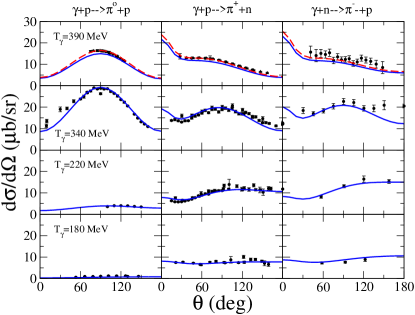
Figure 6 shows the results for differential cross sections for neutral and charged pion productions at various energies together with the data. We see that, overall, the data are reproduced quite well. The dashed curves in the top row correspond to the results represented by the solid curves multiplied by an arbitray factor of 1.1. They are shown here to facilitate visualizing that the shape of the angular distribution is well reproduced, in spite of the absolute normalization being underestimated at this energy by $\sim 10\%$, as can be seen better in Fig. 5.

IV Summary

By exploiting the generalized Ward-Takahashi identity for the production amplitude and total charge conservation, we have constructed a fully gauge-invariant (pseudoscalar) meson photoproduction amplitude which includes the hadronic final-state interaction explicitly. The method is based on a field-theoretical approach developed earlier by Haberzettl HH1 . It is quite general and can be readily extended to any other meson photo- and electroproduction reactions. This method should be particularly relevant for the latter reaction.

As an example of application of the present approach, we have calculated both the neutral and charged pion photoproduction processes off nucleons up to about $400$ MeV photon incident energy which illustrates the feasibility of the present method.

Obviously, for a more quantitative calculation, including not only cross sections but also other observables, some of the approximations made in the present feasibility study should either be improved or altogether avoided. In particular, the dressing of the electromagnetic vertices as given by Eq. (6) needs to be carried out. Also, for pion photoproduction, one should constrain the parameters of the present model, if possible at all, by comparing the amplitude of the present approach in the chiral limit with that of the Chiral Perturbation Theory. Work in this direction is in progress.

Acknowledgements.
This work was supported by the COSY Grant No. 41445282 (COSY-58).

Appendix A Transverse contact current

In this appendix, we give the explicit formulas for the coefficients $\alpha_{i}$, $\beta_{i}$, $\delta_{i}$, and $\eta_{i}$ appearing in Eq. (41). They are

$\displaystyle\alpha_{0}$ $\displaystyle=N\left[a_{1}G+a_{3}\frac{\omega_{q}}{m}+a_{4}\left(\frac{I}{m}-2G\right)\right]\ ,$ (55a)
$\displaystyle\alpha_{1}$ $\displaystyle=N\left[-a_{1}JG-a_{3}\left(1+\omega_{q}H\right)+a_{4}\left(1-IH-2JG\right)\right]\ ,$ (55b)
$\displaystyle\alpha_{2}$ $\displaystyle=N\left[a_{3}-a_{4}\right]mH\ ,$ (55c)

where $\omega_{q}\equiv\sqrt{\vec{q}^{\;2}+m_{\pi}^{2}}$ and

$\displaystyle N$ $\displaystyle\equiv\sqrt{\frac{\varepsilon_{q}+m}{2m}}\sqrt{\frac{\varepsilon_{k}+m}{2m}}\frac{1}{m}\ ,$ (56a)
$\displaystyle G$ $\displaystyle\equiv 1+\frac{|\vec{k}|}{\varepsilon_{k}+m}\ ,$ (56b)
$\displaystyle H$ $\displaystyle\equiv\frac{|\vec{k}|}{\left(\varepsilon_{q}+m\right)\left(\varepsilon_{k}+m\right)}\ ,$ (56c)
$\displaystyle I$ $\displaystyle\equiv\varepsilon_{k}+|\vec{k}|+\varepsilon_{q}\ ,$ (56d)
$\displaystyle J$ $\displaystyle\equiv\frac{m}{\varepsilon_{q}+m}\ ,$ (56e)

with $\varepsilon_{p}\equiv\sqrt{\vec{p}^{\;2}+m^{2}}$. Furthermore,

$\displaystyle\beta_{1}$ $\displaystyle=N\left[-a_{1}JG+a_{3}\omega_{q}H+a_{4}\left(IH+2JG\right)\right]\ ,$ (57a)
$\displaystyle\beta_{2}$ $\displaystyle=-\alpha_{2}\ ,$ (57b)

and

$\displaystyle\delta_{1}$ $\displaystyle=N\Big{[}-a_{1}JG-a_{2}\frac{|\vec{k}|}{m}K+a_{3}\left(G+\omega_{q}H\right)$ (58a)
$\displaystyle\qquad\mbox{}+a_{4}\left(G-IH-2JG\right)\Big{]}\ ,$
$\displaystyle\delta_{2}$ $\displaystyle=-N\left[a_{3}+a_{4}\right]mH\ ,$ (58b)

with $K\equiv 2(\varepsilon_{k}+m)/(\varepsilon_{q}+m)$, and finally

$$\eta_{2}=N\left[a_{2}K-\left(a_{3}-a_{4}\frac{|\vec{k}|}{m}\right)\left(J-mH\right)\right]\ .$$ (59)

Appendix B Transversality of the dressed $N\Delta\gamma$ vertex

For completeness, in this appendix we show how to dress the $N\Delta\gamma$ transition vertex in the present approach and demonstrate that the resulting vertex is purely transverse as it should be.

Bare transition currents can easily be made transverse by expanding the current in an appropriate transverse operator base. It is not obvious, however, that the transversality will remain true after one dresses the current. It will be shown here that this is indeed the case. As a specific example, we will treat the electromagnetic current for the $N\to\Delta$ transition.

Refer to caption

Figure 7: (Color online) Dressed transition current for $\gamma N\to\Delta$. Solid circles depict dressed vertices and currents, whereas open circles show the corresponding bare quantities. The two equivalent forms differ by whether the initial $\pi NN$ vertex or the final $\pi N\Delta$ vertex is fully dressed. Contributions with intermediate particles other than pions and nucleons are not shown.

The dressing mechanism for this current is depicted in Fig. 7 which is constructed in analogy to the dressed nucleon current in (6) (see also Ref. HH1 for full detail). We will consider here only dressing mechanisms in terms of nucleons and pions. Other particles are independent from the ones considered here and formally would not add anything new except complicating the presentation. The two equivalent forms arise from attaching the photon in all possible ways to two equivalent bubbles shown in Fig. 8. It should be obvious, however, that as a physical process the transition $N\to\Delta$ as shown in this figure is not possible because of isospin conservation. Within the present context, therefore, the bubbles in Fig. 8 form but the topological backdrop against which the current shown in Fig. 7 is constructed but are not considered as having a physical meaning of their own.

Refer to caption

Figure 8: (Color online) Topological structure of the bubbles underlying the construction of the transition current in Fig. 7. The first equality follows from the fact that the dressing for both bubbles is done in terms of the non-polar $\pi N$ $T$-matrix $X$ and both bubbles with dressed vertices, therefore, can be written in terms of the graphs of the second line. Taken as a physical process, the transition $N\to\Delta$ is not possible either on or off-shell because of isospin conservation.

Following Ref. js72 , the most general transverse current for

$$\gamma(k)+N(p)\to\Delta(p^{\prime})$$ (60)

may be written as

$\displaystyle\Gamma^{\beta\mu}$ $\displaystyle=G_{1}\,\gamma_{5}\left(k^{\beta}\gamma^{\mu}-g^{\beta\mu}\,{k\!\!\!/}\right)$
$\displaystyle\qquad\mbox{}+G_{2}\,\gamma_{5}\left(k^{\beta}P^{\mu}-g^{\beta\mu}\,k\!\cdot\!P\right)$
$\displaystyle\qquad\quad\mbox{}+G_{3}\,\gamma_{5}\left(k^{\beta}k^{\mu}-g^{\beta\mu}\,k^{2}\right)~{},$ (61)

where $P=(p+p^{\prime})/2=(2p+k)/2$; the Lorentz indices $\mu$ and $\beta$ pertain to the photon and the $\Delta$, respectively. The $G_{i}$ are the corresponding form factors; for real photons, only $G_{1}$ and $G_{2}$ contribute. This is the ansatz that one chooses for the bare current.

To show that the transversality of the bare current is preserved if one now dresses the current, we use the first form of the current shown in Fig. 7. Using the notation of Ref. HH1 , we can translate this into the schematic equation

$\displaystyle\Gamma^{\beta\mu}$ $\displaystyle=\Gamma_{0}^{\beta\mu}+\langle f^{\beta\mu}|S_{N}\circ\Delta_{\pi}|F\rangle$
$\displaystyle\qquad\quad\mbox{}+\langle f^{\beta}|S_{N}\circ\Delta_{\pi}|M^{\mu}_{\text{int}}\rangle$
$\displaystyle\qquad\quad\mbox{}+\langle f^{\beta}|S_{N}\circ[\Delta_{\pi}\Gamma^{\mu}_{\pi}\Delta_{\pi}]|F\rangle$
$\displaystyle\qquad\quad\mbox{}+\langle f^{\beta}|[S_{N}\Gamma^{\mu}_{N}S_{N}]\circ\Delta_{\pi}|F\rangle~{},$ (62)

where the order of terms is exactly as in Fig. 7. The (transverse) bare current is denoted by $\Gamma_{0}^{\beta\mu}$; $f^{\beta}$ is the bare $\pi\Delta N$ vertex and $f^{\beta\mu}$ the corresponding bare contact current. The latter are given by

$$f^{\beta}=f_{\Delta}\,\theta^{\beta\nu}q_{\nu}~{},$$ (63)

where $q_{\nu}$ is the incoming pion momentum, $\theta^{\beta\nu}$ the coupling tensor, and $f_{\Delta}$ the bare coupling constant, and by

$$f^{\beta\mu}=-f_{\Delta}\,\theta^{\beta\mu}e_{\pi}~{},$$ (64)

where $e_{\pi}$ is the charge of the intermediate pion. $F$ is the dressed $\pi NN$ vertex and $M^{\mu}_{\text{int}}$ the corresponding dressed interaction current. The convolution of the intermediate pion and nucleon propagators (with and without attached photons) is denoted by $A\circ B$. The momentum dependence is suppressed here, but can easily be found by noting that the initial nucleon momentum is $p$ and that the photon feeds a momentum $k$ into the line (or vertex) to which it is attached.

Using the Ward–Takahashi identities for the pion, the nucleon, and the interaction current,

$\displaystyle k_{\mu}S_{N}\Gamma^{\mu}_{N}S_{N}$ $\displaystyle=e^{\prime}_{N}\left(\bullet S_{N}-S_{N}\bullet\right)~{},$ (65a)
$\displaystyle k_{\mu}\Delta_{\pi}\Gamma^{\mu}_{\pi}\Delta_{\pi}$ $\displaystyle=e_{\pi}\left(\bullet\Delta_{\pi}-\Delta_{\pi}\bullet\right)~{},$ (65b)
$\displaystyle k_{\mu}M^{\mu}_{\text{int}}$ $\displaystyle=-F[\bullet e_{N}]+[e^{\prime}_{N}\bullet]F+[e_{\pi}\bullet]F~{},$ (65c)

respectively, where the solid dot ($\bullet$) indicates at which point the photon momentum is injected into the equations. For example,

$$e^{\prime}_{N}\left(\bullet S_{N}-S_{N}\bullet\right)=e^{\prime}_{N}\Big{[}S_{N}(p^{\prime\prime})-S_{N}(p^{\prime\prime}+k)\Big{]}~{},$$ (66)

where $p^{\prime\prime}$ is the initial momentum of the nucleon with charge $e^{\prime}_{N}$ within the loop. The notation $[e_{x}\bullet]$ specifies that the photon momentum is injected into the (incoming or outgoing) particle line with charge $e_{x}$. We now find

$\displaystyle k_{\mu}\Gamma^{\beta\mu}$ $\displaystyle=\underbrace{k_{\mu}\Gamma_{0}^{\beta\mu}}_{=0}-f_{\Delta}e_{\pi}\langle\theta^{\beta\mu}k_{\mu}|S_{N}\circ\Delta_{\pi}|F\rangle$
$\displaystyle\qquad\mbox{}-e_{N}\langle f^{\beta}|S_{N}\circ\Delta_{\pi}|F\rangle\bullet$
$\displaystyle\qquad\mbox{}+e_{\pi}\langle f^{\beta}|S_{N}\circ[\Delta_{\pi}\bullet]|F\rangle$
$\displaystyle\qquad\mbox{}+e^{\prime}_{N}\langle f^{\beta}|[S_{N}\bullet]\circ\Delta_{\pi}|F\rangle$
$\displaystyle\qquad\mbox{}+e_{\pi}\langle f^{\beta}|S_{N}\circ[\bullet\Delta_{\pi}]|F\rangle$
$\displaystyle\qquad\mbox{}-e_{\pi}\langle f^{\beta}|S_{N}\circ[\Delta_{\pi}\bullet]|F\rangle$
$\displaystyle\qquad\mbox{}+e^{\prime}_{N}\langle f^{\beta}|[\bullet S_{N}]\circ\Delta_{\pi}|F\rangle$
$\displaystyle\qquad\mbox{}-e^{\prime}_{N}\langle f^{\beta}|[S_{N}\bullet]\circ\Delta_{\pi}|F\rangle$
$\displaystyle=-f_{\Delta}e_{\pi}\langle\theta^{\beta\mu}k_{\mu}|S_{N}\circ\Delta_{\pi}|F\rangle$
$\displaystyle\qquad\mbox{}-e_{N}\langle f^{\beta}|S_{N}\circ\Delta_{\pi}|F\rangle\bullet$
$\displaystyle\qquad\mbox{}+e_{\pi}\langle f^{\beta}|S_{N}\circ[\bullet\Delta_{\pi}]|F\rangle$
$\displaystyle\qquad\mbox{}+e^{\prime}_{N}\langle f^{\beta}|[\bullet S_{N}]\circ\Delta_{\pi}|F\rangle~{},$ (67)

In the second term, the dot $\bullet$ simply indicates that the overall four-momentum of $\langle f^{\beta}|S_{N}\circ\Delta_{\pi}|F\rangle$ is $p+k$. In the first, third, and fourth terms, the intermediate pion propagator depends on the same loop variable $q$ in all terms, but the left-most vertices have momentum dependencies that can be combined according to

$\displaystyle-f_{\Delta}$ $\displaystyle e_{\pi}\langle\theta^{\beta\mu}k_{\mu}|S_{N}\circ\Delta_{\pi}|F\rangle+e_{\pi}\langle f^{\beta}|S_{N}\circ[\bullet\Delta_{\pi}]|F\rangle$
$\displaystyle+e^{\prime}_{N}\langle f^{\beta}|[\bullet S_{N}]\circ\Delta_{\pi}|F\rangle$
$\displaystyle\quad=f_{\Delta}\Big{[}-e_{\pi}\langle\theta^{\beta\mu}k_{\mu}|+e_{\pi}\langle\theta^{\beta\nu}(q+k)_{\nu}|$
$\displaystyle\qquad\qquad\qquad\qquad\mbox{}+e^{\prime}_{N}\langle\theta^{\beta\nu}q_{\nu}|\Big{]}S_{N}\circ\Delta_{\pi}|F\rangle$
$\displaystyle\quad=f_{\Delta}\left[(e^{\prime}_{N}+e_{\pi})\langle\theta^{\beta\nu}q_{\nu}|\right]S_{N}\circ\Delta_{\pi}|F\rangle$
$\displaystyle\quad=(e^{\prime}_{N}+e_{\pi})\langle f^{\beta}|S_{N}\circ\Delta_{\pi}|F\rangle$
$\displaystyle\quad\mbox{}=e_{N}\langle f^{\beta}|S_{N}\circ\Delta_{\pi}|F\rangle~{},$ (68)

where charge conservation,

$$e_{N}=e_{\pi}+e^{\prime}_{N}~{},$$ (69)

was used. Comparison with the first bubble of Fig. 8 shows that

$$\Sigma^{\beta}_{\Delta N}=\langle f^{\beta}|S_{N}\circ\Delta_{\pi}|F\rangle$$ (70)

is just equal to this topological bubble. Hence we have

$$k_{\mu}\Gamma^{\beta\mu}=e_{N}\Big{[}\Sigma^{\beta}_{\Delta N}(p)-\Sigma^{\beta}_{\Delta N}(p+k)\Big{]}~{}.$$ (71)

As explained above, the $\Sigma^{\beta}_{\Delta N}$ do not describe a physical process and vanish individually. Hence, we have

$$k_{\mu}\Gamma^{\beta\mu}=0$$ (72)

and the dressed current thus is also transverse.

We observe that the present approach for dressing the $N\Delta\gamma$ vertex differs from the dressing mechanism employed in other approaches (see, e.g., Sato ; Pascalutsa ) by the presence of the second diagram on the right-hand-side of the equality in Fig. 7. Note that this term involves the three-particle to one-particle transition, $\gamma\pi N\to\Delta$, and therefore is outside the model space considered in those approaches. We emphasize, however, that the presence of the $\Delta\pi N\gamma$ contact vertex is absolutely necessary for preserving the gauge invariance of the dressed vertex in view of the momentum dependence of the $N\Delta\pi$ vertex as given by Eq. (74e) below. This suggests, of course, that indiscriminate truncation of the model space along particle numbers is not a good dynamical ordering scheme as far as the gauge-invariance condition is concerned.

Appendix C Interactions

Our model for the $s$-, $u$-, and $t$-channel amplitudes $M^{\mu}_{s}$, $M^{\mu}_{u}$ and $M^{\mu}_{t}$, respectively, in Eq. (3) is constructed from the interaction Lagrangian density written as a sum of two terms, ${\cal L}_{\text{int}}={\cal L}_{\text{hadr}}+{\cal L}_{\text{elec}}$, where ${\cal L}_{\text{hadr}}$ denotes the part of the interaction Lagrangian containing only the hadron fields, and ${\cal L}_{\text{elec}}$ contains the electromagnetic interaction with hadrons. For ${\cal L}_{\text{hadr}}$, we have

$${\cal L}_{\text{hadr}}={\cal L}_{NN\pi}+{\cal L}_{NN\rho}+{\cal L}_{NNa_{1}}+{\cal L}_{NN\omega}+{\cal L}_{N\Delta\pi}\ ,$$ (73)

with

$\displaystyle{\cal L}_{NN\pi}$ $\displaystyle=-g_{\pi}\bar{\Psi}\left(\gamma_{5}\left[i\lambda+\frac{1-\lambda}{m+m^{\prime}}\,{\partial\!\!\!/}\right]\vec{\pi}\cdot\vec{\tau}\right)\Psi~{},$ (74a)
$\displaystyle{\cal L}_{NN\rho}$ $\displaystyle=-\frac{g_{\rho}}{2}\;\bar{\Psi}\left(\gamma_{\mu}-\frac{\kappa_{\rho}}{2m_{N}}\sigma_{\mu\nu}\partial^{\nu}\right)\vec{\tau}\cdot\vec{\rho}^{\,\mu}\;\Psi~{},$ (74b)
$\displaystyle{\cal L}_{NN\omega}$ $\displaystyle=-\frac{g_{\omega}}{2}\;\bar{\Psi}\left(\gamma_{\mu}-\frac{\kappa_{\omega}}{2m_{N}}\sigma_{\mu\nu}\partial^{\nu}\right)\omega^{\mu}\;\Psi~{},$ (74c)
$\displaystyle{\cal L}_{NNa_{1}}$ $\displaystyle=g_{a_{1}}\,\bar{\Psi}\,\gamma_{\mu}\gamma_{5}\vec{\tau}\cdot\vec{a}_{1}^{\mu}\,\Psi~{},$ (74d)
$\displaystyle{\cal L}_{N\Delta\pi}$ $\displaystyle=\frac{f_{N\Delta\pi}}{m_{\pi}}\,\bar{\Psi}_{\Delta}^{\mu}\,\vec{T}^{\dagger}\cdot(\partial_{\mu}\vec{\pi})\,\Psi\ +\ \text{H.\,c.}$ (74e)

Here, $\Psi$ and $\Psi_{\Delta}^{\mu}$ denote the nucleon and $\Delta$ fields, respectively, $\vec{\pi}$ the pion field, $\vec{\rho}^{\,\mu}$ the $\rho$-meson, $\omega^{\mu}$ the $\omega$-meson, and $\vec{a}_{1}^{\mu}$ the $a_{1}$-meson fields. The latter is included as the chiral partner of the $\rho$-meson. The vector notation refers to the isospin space. $\vec{T}^{\dagger}$ stands for the isospin 1/2 to 3/2 transition operator. The nucleon and pion masses are denoted by $m_{N}$ and $m_{\pi}$, respectively. The $g_{\pi}$, $g_{\rho}$($\kappa_{\rho}$), $g_{a_{1}}$, $g_{\omega}$($\kappa_{\omega}$) and $f_{N\Delta\pi}$ are the corresponding coupling constants. We use $g_{\pi}=14.4$ and $f_{N\Delta\pi}=0.36$ Oliver . For the $NN\rho$ coupling constants, we use $(g_{\rho}/2)^{2}/4\pi=0.91$ and $\kappa_{\rho}=6.1$ Machleidt , while $(g_{\omega}/2)^{2}/4\pi=11$ and $\kappa_{\omega}=0$ Janssen . The coupling constant $g_{a_{1}}=m_{a_{1}}f_{\pi}/m_{\pi}$, with $m_{a_{1}}\approx 1260$ MeV denoting the mass of the $a_{1}$-meson, has been fixed from the chiral-symmetry considerations following the work of Wess and Zumino Wess .

The electromagnetic interaction Lagrangian density is given by

$\displaystyle{\cal L}_{\text{elec}}$ $\displaystyle={\cal L}_{NN\gamma}+{\cal L}_{NN\pi\gamma}+{\cal L}_{\pi\pi\gamma}+{\cal L}_{\omega\pi\gamma}$
$\displaystyle\qquad\mbox{}+{\cal L}_{\rho\pi\gamma}+{\cal L}_{a_{1}\pi\gamma}+{\cal L}_{N\Delta\gamma}~{},$ (75)

with

$\displaystyle{\cal L}_{NN\gamma}$ $\displaystyle=-e\,\bar{\Psi}\left(\hat{e}\gamma_{\mu}-\frac{\hat{\kappa}}{2m_{N}}\sigma_{\mu\nu}\partial^{\nu}\right)A^{\mu}\;\Psi~{}$ (76a)
$\displaystyle{\cal L}_{NN\pi\gamma}$ $\displaystyle=e\,\frac{f_{\pi}}{m_{\pi}}\,\bar{\Psi}\gamma_{5}\gamma_{\mu}[\vec{\tau}\times\vec{\pi}]_{3}\,\Psi A^{\mu}~{},$ (76b)
$\displaystyle{\cal L}_{\pi\pi\gamma}$ $\displaystyle=e\,[(\partial_{\mu}\vec{\pi})\times\vec{\pi}]_{3}A^{\mu}~{},$ (76c)
$\displaystyle{\cal L}_{\omega\pi\gamma}$ $\displaystyle=e\,\frac{g_{\omega\pi\gamma}}{m_{\pi}}\varepsilon_{\alpha\mu\lambda\nu}\,(\partial^{\alpha}A^{\mu})(\partial^{\lambda}\pi_{3})\omega^{\nu}~{},$ (76d)
$\displaystyle{\cal L}_{\rho\pi\gamma}$ $\displaystyle=e\,\frac{g_{\rho\pi\gamma}}{m_{\pi}}\varepsilon_{\alpha\mu\lambda\nu}\,(\partial^{\alpha}A^{\mu})(\partial^{\lambda}\vec{\pi})\cdot\vec{\rho}^{\,\nu}~{},$ (76e)
$\displaystyle{\cal L}_{a_{1}\pi\gamma}$ $\displaystyle=-e\,\frac{1}{m_{a_{1}}}F_{\mu\nu}$
$\displaystyle\quad\mbox{}\times\biggl{(}2\bigl{[}(\partial^{\mu}\vec{\pi})\times\vec{a}_{1}^{\nu}-(\partial^{\nu}\vec{\pi})\times\vec{a}_{1}^{\mu}\bigr{]}+\vec{\pi}\times\vec{a}_{1}^{\mu\nu}\biggr{)}~{},$ (76f)
$\displaystyle{\cal L}_{N\Delta\gamma}$ $\displaystyle=ie\frac{G_{1}}{2m_{N}}\bar{\Psi}_{\Delta}^{\mu}\,T_{z}^{\dagger}\gamma_{5}\gamma^{\nu}\,\Psi F_{\mu\nu}$
$\displaystyle\quad\mbox{}+e\,\frac{G_{2}}{4m_{N}^{2}}\left(\partial^{\nu}\bar{\Psi}_{\Delta}^{\mu}\right)T_{z}^{\dagger}\gamma_{5}\Psi F_{\mu\nu}+\ \ \text{H.\,c.}~{},$ (76g)

where $F_{\mu\nu}\equiv\partial_{\mu}A_{\nu}-\partial_{\nu}A_{\mu}$ with $A_{\mu}$ denoting the electromagnetic field and $\vec{a}_{1}^{\mu\nu}\equiv\partial^{\mu}\vec{a}_{1}^{\nu}-\partial^{\nu}\vec{a}_{1}^{\mu}$. $e$ is the proton charge; $\hat{e}=(1+\tau_{z})/2$ and $\hat{\kappa}=[1.79(1+\tau_{z})/2-1.93(1-\tau_{z})/2]$ are the charge and magnetic moment operators of the nucleon, respectively. The coupling constants $g_{\omega\pi\gamma}=0.374$ and $g_{\rho\pi\gamma}=0.125$ are fixed from the decay of the $\omega$- and $\rho$-meson into $\pi^{0}+\gamma$, respectively. The signs of these coupling constants are consistent with those determined from the study of pion photo-production in the $1$ GeV region Garc . $\varepsilon_{\mu\alpha\lambda\nu}$ is the totally antisymmetric Levi-Civita tensor with $\varepsilon^{0123}=+1$. The Lagrangian ${\cal L}_{a_{1}\pi\gamma}$ is obtained from ${\cal L}_{a_{1}\pi\rho}$ in Ref. Wess by combining it with the vector-dominance model.

The propagators required for constructing $M^{\mu}_{s}$, $M^{\mu}_{u}$, and $M^{\mu}_{t}$ are

$\displaystyle\Delta_{\pi}(q)$ $\displaystyle=\frac{1}{q^{2}-m_{\pi}^{2}}~{},$ (77a)
$\displaystyle D_{v}^{\mu\nu}(q)$ $\displaystyle=-\frac{g^{\mu\nu}-q^{\mu}q^{\nu}/m_{v}^{2}}{q^{2}-m_{v}^{2}}~{},\quad\text{for}\quad v=\rho,\omega,a_{1}~{},$ (77b)
$\displaystyle S_{N}(p)$ $\displaystyle=\frac{1}{{p\!\!\!/}-m_{N}}~{},$ (77c)
$\displaystyle S_{\Delta}^{\mu\nu}(p)$ $\displaystyle=\frac{{p\!\!\!/}+m_{\Delta}}{p^{2}-m_{\Delta}^{2}}$
$\displaystyle\quad\mbox{}\times\left[-g^{\mu\nu}+\frac{1}{3}\gamma^{\mu}\gamma^{\nu}+\frac{2}{3}\frac{p^{\mu}p^{\nu}}{m_{\Delta}^{2}}-\frac{p^{\mu}\gamma^{\nu}-p^{\nu}\gamma^{\mu}}{3m_{\Delta}}\right]~{},$ (77d)

where $\Delta_{\pi}(q)$ denotes the pion propagator and $D_{v}^{\mu\nu}(q)$ the vector ($\rho$, $\omega$) and axial-vector ($a_{1}$) meson propagators. $S_{N}(p)$ and $S_{\Delta}^{\mu\nu}(p)$ are the nucleon and Rarita-Schwinger $\Delta$ propagators, respectively; $m_{\Delta}=1232$ MeV denotes the mass of the $\Delta$. Note that for the $s$-channel $\Delta$ resonance contribution, we have used the dressed $N\Delta\pi$ vertex and the dressed $\Delta$ propagator according to Ref. Oliver and consistent with the $\pi N$ FSI used.

The amplitudes $M^{\mu}_{s}$, $M^{\mu}_{u}$, and $M^{\mu}_{t}$ constructed from the preceding Lagrangians are diagrammatically represented in Fig. 1(a).

Our model for $M^{\mu}_{s}$, $M^{\mu}_{u}$ and $M^{\mu}_{t}$ is supplemented with hadronic form factors, except for the $s$-channel $\Delta$ contribution where the dressed vertex is used. So, the $NN\pi$ vertex in the $s$- and $u$-channels and the $N\Delta\pi$ vertex in the $u$-channel are multiplied by a form factor

$$F_{B}(\vec{p}\ ^{2})=\frac{\Lambda_{B}^{4}}{\Lambda_{B}^{4}+(\vec{p}\ ^{2}+m_{B}^{2})^{2}}\ ,$$ (78)

where $\vec{p}$ denotes the three-momentum of the off-shell baryon. In the above equation $B$ stands for either the nucleon or $\Delta$ in the intermediate state. We take $\Lambda_{B}=1.2$ GeV for both baryons.

The hadronic vertices in the $t$-channel $M^{\mu}_{t}$ amplitude are also supplemented by form factors of the form

$$F_{\alpha}(q^{2})=\left(\frac{\Lambda_{\alpha}^{2}-m_{\alpha}^{2}}{\Lambda_{\alpha}^{2}-q^{2}}\right)^{n_{\alpha}}\ ,$$ (79)

where $\alpha=\pi,\rho,\omega,a_{1}$. We take $\Lambda_{\pi}=900$ MeV and $n_{\pi}=1$ Janssen and $\Lambda_{\alpha}=1850$ MeV and $n_{\alpha}=2$ as $\alpha=\rho,\omega,a_{1}$ Machleidt .

References

  • (1) G. F. Chew, M. L. Goldberger, F. E. Low, and Y. Nambu, Phys. Rev. 106, 1345 (1957).
  • (2) V. Bernard, N. Kaiser, J. Gasser and U.-G. Meißner, Phys. Lett. B268, 291 (1991).
  • (3) V. Bernard, N. Kaiser and U.-G. Meißner, Nucl. Phys.  B383, 442 (1992).
  • (4) V. Bernard, N. Kaiser, T.-S. H. Lee, and U.-G. Meißner, Phys. Rep. 246, 315 (1994).
  • (5) V. Bernard, N. Kaiser, and U.-G. Meißner, Phys. Lett. B378, 337 (1996); Phys. Lett. B383, 116 (1996).
  • (6) T. Feuster and U. Mosel, Phys. Rev. C 59, 460 (1999).
  • (7) G. Penner and U. Mosel, Phys. Rev. C 66, 055211 (2002); C 66, 055212 (2002).
  • (8) O. Scholten, A. Yu. Korchin, V. Pascalutsa, and D. van Neck, Phys. Lett. B384, 13 (1996).
  • (9) D. Drechsel, O. Hanstein, S. S. Kamalov, and L. Tiator, Nucl. Phys. A645, 145 (1999).
  • (10) O. Hanstein, D. Drechsel, and L. Tiator, Nucl. Phys. A632, 561 (1998).
  • (11) S. Nozawa, B. Blankleider, and T.-S. H. Lee, Nucl. Phys. A513, 459 (1990); S. Nozawa, T.-S. H. Lee, and B. Blankleider, Phys. Rev. C 41, 213 (1990).
  • (12) Y. Surya and F. Gross, Phys. Rev. C 53 2422 (1996).
  • (13) T. Sato and T.-S. H. Lee, Phys. Rev. C 54, 2660 (1996).
  • (14) V. Pascalutsa and J. A. Tjon, Phys. Rev. C 70, 035209 (2004).
  • (15) F. Gross and D. O. Riska, Phys. Rev. C 36, 1928 (1987).
  • (16) K. Ohta, Phys. Rev. C 40, 1335 (1989).
  • (17) C. H. M. van Antwerpen and I. Afnan, Phys. Rev. C 52, 554 (1995).
  • (18) H. Haberzettl, Phys. Rev. C 56, 2041 (1997).
  • (19) H. Haberzettl, C. Bennhold, T. Mart, and T. Feuster, Phys. Rev. C 58, R40 (1998).
  • (20) A. N. Kvinikhidze and B. Blankleider, Phys. Rev. C 60, 044003 (1999); ibid., 044004 (1999).
  • (21) R. M. Davidson and R. Workman, Phys. Rev.  C 63, 025210 (2001).
  • (22) B. Borasoy, P. C. Bruns, U.-G. Meißner and R. Nissler, Phys. Rev. C 72, 065201 (2005).
  • (23) A. Usov and O. Scholten, Phys. Rev. C 72, 025205 (2005).
  • (24) S. Nozawa and T.-S. H Lee, Nucl. Phys. A513, 511 (1990).
  • (25) G. L. Caia, V. Pascalutsa, J. A. Tjon, and L. E. Wright, Phys. Rev. C 70, 032201(R) (2004); G. L. Caia, L. E. Wright, and V. Pascalutsa, Phys. Rev. C 72, 035203 (2005).
  • (26) E. Kazes, Nuovo Cimento 13, 1226 (1959).
  • (27) F. de Jong and K. Nakayama, Phys. Lett. B385, 33 (1996).
  • (28) H. Haberzettl, Phys. Rev. C 62, 034605 (2000).
  • (29) K. Nakayama and W. G. Love, Phys. Rev. C 72, 034603 (2005).
  • (30) O. Krehl, C. Hanhart, S. Krewald, and J. Speth, Phys. Rev. C 62, 025207 (2000).
  • (31) S. S. Schweber, An Introduction to Relativistic Quantum Field Theory, (Harper & Row, New York, NY, 1962; reprinted by Dover, Minealo, NY, 2005).
  • (32) G. Blanpied et al., Phys. Rev. Lett. 79, 4337 (1998).
  • (33) R. Beck et al., Phys. Rev. C 61, 035204 (2000).
  • (34) E. Mazzucato et al., Phys. Rev. Lett. 57, 3144 (1986); R. Beck et al., Phys. Rev. Lett. 65, 1841 (1990); M. Fuchs et al., Phys. Lett. B368, 20 (1996); J. C. Bergstrom et al., Phys. Rev. C 53, 1052 (1996); A. Schmit et al., Phys. Rev. Lett. 87, 232501 (2001); B. B. Govorkov et al., Sov. J. Nucl. Phys. 6, 370 (1968); W. Hitzeroth et al., Nuovo Cimento A 60, 467 (1969); J. Ahrens et al., Phys. Rev. Lett. 84, 5950 (2000); R. G. Vasilkov et al., JETP 10, 7 (1960); F. Härter, PhD Thesis, Johannes-Gutenberg Universität Mainz (1996); M. MacCormick et al., Phys. Rev. C 53, 41 (1996).
  • (35) D. Menze, W. Pfeil, and R. Wilcke, ZAED Compilation of Pion Photoproduction Data, University of Bonn, 1977; M. Yoshioka et al., Nucl. Phys. B168, 222 (1980); J.-L. Faure et al., Nucl. Phys. A424, 383 (1984); R. Beck et al., Phys. Rev. Lett. 78, 606 (1997); J. Ahrens et al., Eur. Phys. J. A21, 323 (2004); A. Shafi et al., Phys. Rev. C 70, 035204 (2004);
  • (36) H. F. Jones and M. D. Scadron, Ann. of Phys. 81, 1 (1972).
  • (37) R. Machleidt, K. Holinde, and Ch. Elster, Phys. Rep. 149, 1 (1987).
  • (38) G. Janssen, K. Holinde, and J. Speth, Phys. Rev. Lett. 73, 1332 (1994); Phys. Rev. C 49, 2763 (1994).
  • (39) J. Wess and B. Zumino, Phys. Rev. 163, 1727 (1967).
  • (40) H. Garcilazo and E. Moya de Guerra, Nucl. Phys. A562, 521 (1993).