Hadron production from resonance decay in relativistic collisions

Abstract

A statistical model for decay and formation of heavy hadronic resonances is formulated. The resonance properties become increasingly uncertain with increasing resonance mass. Drawing on analogy with the situation in low-energy nuclear physics, we employ the Weisskopf approach to the resonance processes. In the large-mass limit, the density of resonance states in mass is governed by a universal Hagedorn-like temperature $T_{H}$. As resonances decay, progressively more and more numerous lighter states get populated. For $T_{H}\simeq 170\,\mbox{MeV}$, the model describes data for the hadron yield ratios at the RHIC and SPS energies under the extreme assumption of a single heavy resonance giving rise to measured yields.

Studies of ultrarelativistic nuclear reactions aim at learning on properties of highly-excited strongly-interacting matter and, in particular, on the predicted transition to quark-gluon plasma (QGP) qm2004 ; gyulassy . Yields from those reactions can be described in terms of grand-canonical thermodynamic models braun ; redlich ; becattini ; braun1 , at temperatures close to those anticipated for the transition karsch . Similar temperatures are utilized in the microcanonical model for electron-positron annihilation into hadrons ep . Large fractions of final light-particles within those thermodynamic equilibrium models result from secondary decays of heavy resonances whose features are, generally, less and less known the heavier the resonances. The lack of knowledge has forced the use of cut-offs on the primary resonance mass in equilibrium models braun ; redlich ; becattini ; braun1 ; analogous cut-offs have been employed in transport models urqmd ; hsd ; ampt . In this paper, we explore the possibility of an apparent equilibrium in the reactions stemming from sequential binary decays of heavy resonances, with the characteristic temperature describing the resonance mass spectrum, rather than being proposed ad hoc.

The situation of deteriorating knowledge of resonance properties, with increasing resonance energy and resonance density in energy, reminisces that of resonances in low-energy nuclear physics. There, statistical descriptions, in terms of the Weisskopf compound-nucleus model and the Hauser-Feschbach theory, have been highly successful statmod . Underlying the statistical descriptions is the density of resonance states in energy $\rho(m,q)$, where $q$ represents discrete quantum numbers of the resonances. For the hadronic states, a universal temperature in terms of the density of states, $T_{H}^{-1}=\partial\log{\rho}/\partial m$, has been originally considered by Hagedorn hagedorn , in part due to an evidence for a rapid, nearly exponential, increase in the number of resonances with energy; see also broniowski . To reach a conclusion on the basis of spectrum, however, the counting of resonances should be carried out at constant values of the quantum numbers $q$, particularly in the region of opening thresholds for different $q$. This has not been considered in Refs. hagedorn ; broniowski . Nonetheless, in the limit of large $m$ at fixed $q/m$, the universal temperature $T_{H}$, independent of $m$, but possibly dependent on $q/m$, may be expected for the resonances due to the lack of any scales that could govern the $T_{H}$-dependence on $m$. While our model for $\rho$ will be fairly schematic, similar to the models employed in the literature hagedorn ; broniowski , there are generally important questions regarding strong interactions that can be suitably asked in terms of $\rho$, concerning e.g., besides the $T_{H}(q/m)$ dependence, the emergence of a surface tension in the thermodynamic limit. In the context of the phase transition, the temperature $T_{H}$ may be considered as the temperature for a metastable equilibrium of quark-gluon drops with vacuum, and, as such, slightly lower temperature than the critical $T_{c}$.

For resonances described by the continuum density of states $\rho$, we consider the processes of binary breakup and inverse fusion, constrained by detailed balance, geometry and by the conservation of baryon number $B$, strangeness $S$, isospin $I$ and of isospin projection $I_{z}$. From the two versions of our model, with and without a strict conservation of angular momentum $(J,J_{z})$, we discuss the simpler Weisskopf version, in this first model presentation. The lighter particles (comprising of 55 baryonic and 34 mesonic states) are treated explicitly as discrete states in the model. Our model allows to explore various aspects of the system evolution in ultrarelativistic collisions, including formation of hadrons with extreme strangeness and isospin, as well as chemical and kinetic freeze-out.

We first discuss details of the density of states. As a threshold mass, separating the discrete states from those in the statistical continuum, we take $m_{\rm th}^{c}=2\,\mbox{GeV}$. We assume that at low excitation energies the density of states is similar at different $q$ for the same excitation energy above the spectrum bottom $m_{g}(q)$. Following quark considerations, we adopt

$$m_{g}(q)=a_{Q}\,{\rm max}\left(|3B+S|,2I\right)+a_{S}\,|S|\,,$$ (1)

where $a_{Q}=0.387\,\mbox{GeV}$ and $a_{S}=0.459\,\mbox{GeV}$. The coefficient magnitudes have been adjusted requiring that the mass $m_{g}(q)$ from Eq. (1) exceeds the lowest known masses for different $q$; regarding the practicality of sequential decays, we prefer to overestimate rather than to underestimate the reference position of spectrum bottom for the continuum, and to overestimate its rise with $q$, to preclude the emergence of any unphysical stable states towards the continuum bottom. At high masses $m$ the influence of the ground state mass on $\rho$ should decrease. We eventually arrive at the following density of states employed in our calculations:

$$\rho(m,q)=A\,\frac{\exp\!\left[\left\{m-m_{g}\,f(m-m_{g})\right\}/T_{H}\right]}{\left[\left\{m-m_{g}\,f(m-m_{g})\right\}^{2}+m_{r}^{2}\right]^{\alpha}}\,.$$ (2)

The role of the factor $f$ is to suppress the effect of $m_{g}$ at high $m$ and we use

$$f(m-m_{g})=\frac{1}{1+\left[(m-m_{g})/m_{\rm th}^{c}\right]^{n}}\,.$$ (3)

with $n=1$. The prefactor of the exponential in Eq. (2), with $m_{r}=0.5\,\mbox{GeV}$, acts to enhance asymmetric (rather than symmetric) breakups for continuum hadrons, leaving the issue of surface tension in the thermodynamic limit open. The normalizing factor $A$ and the power $\alpha$ are adjusted, for different assumed values of Hagedorn temperature $T_{H}$, by comparing the low-$m$ cumulant spectra from measurements and from the continuum representation broniowski :

$$N_{\rm exp} = \sum_{i}(2J+1)\,\Theta(m-m_{i})\,,$$

$$N_{\rm the} = \sum_{q}\int^{m}{\rm d}m^{\prime}\,\rho(m^{\prime},q)\,.$$ (4)

For $T_{H}=170$ MeV, as an example, we obtain the prefactor power of $\alpha=2.82$. The normalization factor $A$ drops out from probabilities for the most common processes involving continuum hadrons, with one continuum and one discrete hadron either in the initial or final state.

We now turn to cross sections and decay rates. The cross section for the formation of a resonance $q$ in the interaction of hadrons 1 and 2, can be, on one hand, represented as danielewicz :

$$\sigma(q_{1}+q_{2}\to q) = \frac{1}{v_{12}}\,\frac{m_{1}}{e_{1}({\bf p}_{1})}\,\frac{m_{2}}{e_{2}({\bf p}_{2})}\int\frac{{\rm d}{\bf p}}{(2\pi)^{3}}\int\frac{{\rm d}e}{2\pi}\,2\pi\,\rho(m,q)\,|{\cal M}_{q_{1}+q_{2}\to q}|^{2}$$ (5)

$$\times(2\pi)^{3}\,\delta\left({\bf p}_{1}+{\bf p}_{2}-{\bf p}\right)2\pi\,\delta\left(e_{1}({\bf p}_{1})+e_{2}({\bf p}_{2})-e\right)$$

$$= \frac{2\pi\,m_{1}\,m_{2}}{m\,p^{\star}(m_{1},m_{2})}\,\rho(m,q)\,|{\cal M}_{q_{1}+q_{2}\to q}|^{2}\,.$$

Here, $v_{12}$ is the relative velocity, $e$’s are the single-particle energies, and $|{\cal M}|^{2}$ is the matrix element squared for the fusion, which is averaged over initial and final spin directions. The factor of $(2J+1)$, associated with the last averaging, has been absorbed into $\rho$. The c.m. momentum in Eq. (5) is

$$p^{\star}(m_{a},m_{b})=\frac{1}{2m}\left[\left(m^{2}-(m_{a}+m_{b})^{2}\right)\left(m^{2}-(m_{a}-m_{b})^{2}\right)\right]^{1/2}\,.$$ (6)

For the final state in continuum, following geometric considerations, the cross section for fusion, on the other hand, is

$$\sigma(q_{1}+q_{2}\to q)=\langle I_{1}\,I_{z_{1}}\,I_{2}\,I_{z_{2}}||I\,I_{z}\rangle\,\pi\,R^{2}\,,$$ (7)

where $\langle\cdot||\cdot\rangle$ represents the isospin Clebsch-Gordan coefficient. The cross section radius is taken as that of the fused entity, $R\approx r_{0}\,(m/m_{d})^{1/3}$, with $r_{0}=1\,\mbox{fm}$ as a characteristic radius for a $m_{d}=1\,\mbox{GeV}$ hadron. Equations (5) and (7) allow to extract the square of the transition matrix element needed for computation of the partial resonance-width.

The partial width for decay into $q_{1}$ and $q_{2}$ can be generally represented as

$$\Gamma(q\to q_{1}+q_{2}) = \int\frac{{\rm d}{\bf p}}{(2\pi)^{3}}\int{\rm d}m_{1}^{\prime}\,\frac{m_{1}^{\prime}\,\rho(m_{1}^{\prime},q_{1})}{e_{1}({\bf p})}\int{\rm d}m_{2}^{\prime}\,\frac{m_{2}^{\prime}\,\rho(m_{2}^{\prime},q_{2})}{e_{2}({\bf p})}$$ (8)

$$\times|{\cal M}_{q\to q_{1}+q_{2}}|^{2}\,2\pi\,\delta\left(e_{1}({\bf p})+e_{2}({\bf p})-m\right)\,.$$

As before, the factors of $(2J_{j}+1)$ are absorbed into $\rho_{j}$. A resonance in the continuum can undergo three types of binary decay: where (i) both daughters are particles with well established properties within the discrete spectrum below $m_{\rm th}^{c}=2\,\mbox{GeV}$, (ii) one of the daughters belongs to the discrete spectrum and the other to the continuum and, finally, where (iii) both daughter resonances belong to the continuum. In the case (i), the state densities are $\rho_{j}(m_{j}^{\prime})=(2J_{j}+1)\,\delta(m_{j}^{\prime}-m_{j})$. With the detailed balance relation, $|{\cal M}_{q\to q_{1}+q_{2}}|^{2}=|{\cal M}_{q_{1}+q_{2}\to q}|^{2}$, we then get

$$\Gamma^{(i)}(q\to q_{1}+q_{2}) = \frac{m_{1}\,m_{2}\,p^{\star}(m_{1},m_{2})}{\pi\,m}\,(2J_{1}+1)\,(2J_{2}+1)\,|{\cal M}_{q\to q_{1}\,q_{2}}|^{2}$$ (9)

$$= \langle I_{1}\,I_{z_{1}}\,I_{2}\,I_{z_{2}}||I\,I_{z}\rangle\,\frac{(2J_{1}+1)\,(2J_{2}+1)\,p^{\star 2}(m_{1},m_{2})\,R^{2}}{2\pi\,\rho(m,q)}\,.$$

In analyzing the case (ii), let the particle characterized by $q_{1}$ belong to the discrete spectrum and that characterized by $q_{2}$ to the continuum spectrum. From (8), we then find

$$\Gamma^{(ii)}(q\to q_{1}+q_{2}) = \langle I_{1}\,I_{z_{1}}\,I_{2}\,I_{z_{2}}||I\,I_{z}\rangle\,\frac{(2J_{1}+1)\,m\,R^{2}\,}{2\pi\,\rho(m,q)}$$ (10)

$$\times\int_{0}^{p^{*}(m_{1},m_{c_{2}})}{\rm d}p\,\frac{p^{3}\,\rho(\sqrt{m^{2}+m_{1}^{2}-2m\,e_{1}},q_{2})}{e_{1}\,\sqrt{m^{2}+m_{1}^{2}-2m\,e_{1}}}\,,$$

where $m_{c_{2}}=\mbox{max}(m_{\rm th}^{c},m_{g}(q_{2}))$. For $e_{1}$ small compared to $m$, it is of advantage to represent the subintegral density of states as an exponential of the density logarithm and to expand the logarithm in $(e_{1}-m_{1})$. The integration over relative momentum can be thereafter carried out explicitly, yielding

$$\Gamma^{(ii)}(q\to q_{1}+q_{2})=\langle I_{1}\,I_{z_{1}}\,I_{2}\,I_{z_{2}}||I\,I_{z}\rangle\,\frac{(2J_{1}+1)\,mR^{2}\,T_{2}^{2}\,(T_{2}+m_{1})}{\pi\,m_{2}}\,\frac{\rho(m_{2},q_{2})}{\rho(m,q)}\,.$$ (11)

Here, $m_{2}=m-m_{1}$ and the temperature is defined as

$$\frac{1}{T_{2}} = \frac{m}{m_{2}}\,\frac{\partial\,\log{\rho(m_{2},q_{2})}}{\partial m_{2}}$$ (12)

$$\approx \frac{m}{m_{2}\,T_{H}}\,\left\{1+\frac{n\,(m^{c}_{\rm th})^{n}\,\left[m_{2}-m_{g}(q_{2})\right]^{n-1}}{(m^{c}_{\rm th})^{n}+\left[m_{2}-m_{g}(q_{2})\right]^{n}}\right\}\,.$$

For $(m_{1},q_{1})$ small compared to $(m,q)$, the obvious further possibility is the expansion of $\log{\rho(m_{2},q_{2})}$ in $(m_{1},q_{1})$, with an emergence of the chemical potentials conjugate to $q_{2}$.

In the case (iii), of both daughters in the continuum with large masses $m_{i}>m_{th}^{c}=2\,\mbox{GeV}$, the nonrelativistic limit in Eq. (8) is justified. On employing Eqs. (5) and (7), the result for the partial width is

$$\Gamma^{(iii)}(q\to q_{1}+q_{2}) = \langle I_{1}\,I_{z_{1}}\,I_{2}\,I_{z_{2}}||I\,I_{z}\rangle\,\frac{m\,R^{2}}{8\pi\,\rho(m,q)}\,\int_{0}^{m-m_{c_{1}}-m_{c_{2}}}{\rm d}\epsilon\,\epsilon\,\overline{\rho}(m-\epsilon,q_{1},q_{2})$$ (13)

$$= \langle I_{1}\,I_{z_{1}}\,I_{2}\,I_{z_{2}}||I\,I_{z}\rangle\,\frac{m\,R^{2}\,T_{12}^{2}}{8\pi}\,\frac{\overline{\rho}(m,q_{1},q_{2})}{\rho(m,q)}\,,$$

where

$$\overline{\rho}(m,q_{1},q_{2})=\int_{2m_{c_{1}}-m}^{m-2m_{c_{2}}}{\rm d}u\,\rho\left({(m+u)}/{2},q_{1}\right)\,\rho\left({(m-u)}/{2},q_{2}\right)\,\left(1-{u^{2}}/{m^{2}}\right)\,.$$ (14)

To obtain the last expression in Eq. (13), we have expanded the logarithm of subintegral density, with the temperature representing $1/T_{12}=\partial[\log\overline{\rho}(m,q_{1},q_{2})]\big{/}\partial m$.

The total decay width of an $(m,q)$ resonance is finally

$$\Gamma(m,q)=\sum_{q_{1}\,q_{2}}\Gamma^{(i)}(q\to q_{1}+q_{2})+\sum_{q_{1}\,q_{2}}\Gamma^{(ii)}(q\to q_{1}+q_{2})+\sum_{q_{1}\,q_{2}}\Gamma^{(iii)}(q\to q_{1}+q_{2})\,.$$ (15)

A moving resonance will live an average time of $\langle\tau\rangle=\gamma/\Gamma$, where $\gamma$ is the resonance Lorentz factor.

The formulas above provide the basis for our Monte-Carlo simulations of the resonance decay sequences in heavy ion collisions. A resonance follows an exponential decay law corresponding to $\langle\tau\rangle$. The product properties are selected according to the decay branching ratios. Since the parent angular momentum is not tracked in the Weisskopf approach, the angular distribution of products is taken as isotropic. During the evolution two resonances can fuse with each other, according to the cross section of Eq. (7), if the final state is in continuum. If, on the other hand, the state is discrete, the cross section acquires the standard form danielewicz , from Eqs. (5) and (9),

$$\sigma(q_{1}+q_{2}\to q)=\frac{2\pi^{2}\,\rho(m,q)\,\Gamma(q\to q_{1}+q_{2})}{(2J_{1}+1)\,(2J_{2}+1)\,p^{\star 2}(m_{1},m_{2})}\,,$$ (16)

where the width for the spectral function is considered:

$$\rho(m,q)=\frac{(2J+1)\,2m_{q}^{2}\,\Gamma}{\pi\left[(m^{2}-m_{q}^{2})^{2}+m_{q}^{2}\,\Gamma^{2}\right]}\approx\frac{(2J+1)\,\Gamma}{2\pi\left[(m-m_{q})^{2}+\Gamma^{2}/4\right]}\,.$$ (17)

Besides the decay and fusion processes, related by detailed balance, a provisional constant cross section $\sigma_{\rm el}=5$ mb has been assumed for all collisions.

In our model, we simulate, in particular, the features of the final state of central Au+Au collisions at $\sqrt{s}=130A$ GeV. Following the presumption that the decay sequences will tend to erase fine details of the initial state, we push the characteristics of the initial state to an extreme, allowing for a single heavy resonance to populate a given rapidity region. In the end, when examining the transverse momentum spectra, we find that the resonance decay and reformation alone generates insufficient transverse collective energy, indicating that the early resonances need to be affected by a collective motion generated prior to the resonance stage. This finding is consistent with those in other works braun ; heinz .

Within the single resonance scenario, the local final state reflects the initial quantum numbers of a resonance characterized by $(m_{0},q_{0})$, where $q_{0}\equiv(B_{0},S_{0},I_{0},I_{z\,0})$. After the value of the Hagedorn temperature $T_{H}$ is set, the relative yields of particles in the final state are, in practice, sensitive only to the relative values of the quantum numbers of the initial resonance. We normally impose strangeness neutrality, so that the starting value is $S_{0}=0$. The magnitude of $B_{0}$, for a given $m_{0}$, can be adjusted by using the final-state antiproton-to-proton or antiproton-to-pion ratios. The starting isospin, for a given $B_{0}$, can be adjusted by using the isospin of original nuclei. However, we find that the initial isospin has only a marginal impact on the isospin of individual final particles. This may be attributed to the cumulative effect of isospin fluctuations when many particles, compared to $I$, are produced. For specific initial $(m_{0},q_{0})$ values, we repeat numerous times the Monte-Carlo simulations of the decay chain and recombination, and the results presented here are an average of about $10^{4}$ generated event sequences.

Figure 1 illustrates the average features of an exemplary local system that starts out as a resonance characterized by $m_{0}=100$ GeV and $B_{0}=3$. The left panel shows the ratio of the average maximal resonance mass $m_{\rm max}$ to the initial mass $m_{0}$, as a function of time, as well as the mass asymmetry, the mass difference between the heaviest resonance and the next heaviest, divided by the sum of their masses, $a_{2}=(m_{\rm max}-m_{2})/(m_{\rm max}+m_{2})$. Persistence of the large asymmetry with time indicates that the heavy resonance decays primarily through light-hadron emission.

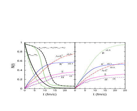
Figure 1: Time evolution of average characteristics for a system starting at $m_{0}=100$ GeV, $B_{0}=3$ and $S_{0}=0$, under the assumption of $T_{H}=170$ MeV. Displayed in the left panel is the ratio of the maximal resonance mass to the initial resonance mass, $m_{\rm max}/m_{0}$, as well as the mass asymmetry, $a_{2}=(m_{\rm max}-m_{2})/(m_{\rm max}+m_{2})$, where $m_{2}$ is the mass of the second heaviest resonance. These results are shown both for the standard system evolution, then represented by the monotonically dropping solid and dashed lines, and for the evolution with suppressed fusion reactions, then represented by the monotonically dropping dash-dotted and dotted lines, respectively. In addition, the left and right panel display the evolution of particle and antiparticle abundances, respectively, for the standard evolution, in terms of rising lines.

In addition, Fig. 1 shows, as a function of time, the abundances of particles (left panel) and antiparticles (right panel). The antibaryon abundances freeze out noticeably earlier than the baryon abundances, in spite of a low initial baryon number relative to the initial mass. The higher the strangeness, the later the abundance saturates. This is likely due to the fact that the effects of strangeness fluctuation need to accumulate with time; the situation would change if we assumed strangeness fluctuations right for the initial resonance conditions.

The calculations have been repeated while suppressing the back resonance fusion reactions. As expected, in this case the maximal mass and asymmetry decrease faster with time, see the left panel of Fig. 1. The abundances (not shown) grow faster and saturate earlier for the modified evolution.

Table 1: Particle yield ratios from the resonance decay model compared to the RHIC Au+Au central-collision data at $\sqrt{s}=130\,A$ GeV. In the model, the starting baryon number of $B_{0}=3$ is assumed, and the mass of either $m_{0}=100$ GeV or $m_{0}=95$ GeV with a corresponding resonance mass spectrum temperature of either $T_{H}=170$ MeV or $T_{H}=175$ MeV is used. Results obtained when suppressing fusion reactions, for $T_{H}=170$ MeV, are provided in parenthesis.

Yield-Ratio	Decay-Model Results		Experimental	Collaboration	Ref.
	$T_{H}=170$ MeV	$175$ MeV	Data
$\overline{p}/\pi^{-}$	0.06 (0.05)	0.07	0.07 $\pm$ 0.01	STAR	olga
$\pi^{-}/\pi^{+}$	1.01 (1.01)	1.01	1.00 $\pm$ 0.02	PHOBOS	ratioph
			0.95 $\pm$ 0.06	BRAHMS	bearden
$K^{+}/K^{-}$	1.073 (1.078)	1.074	1.092 $\pm$ 0.023	STAR	kpkmst
			1.28 $\pm$ 0.13	PHENIX	zajc
			1.09 $\pm$ 0.09	PHOBOS	ratioph
			1.12 $\pm$ 0.07	BRAHMS	bearden
$K^{-}/\pi^{-}$	0.175 (0.185)	0.175	0.146 $\pm$ 0.024	STAR	kpist
$\overline{p}/p$	0.65 (0.63)	0.66	0.65 $\pm$ 0.07	STAR	pbpst
			0.64 $\pm$ 0.07	PHENIX	zajc
			0.60 $\pm$ 0.07	PHOBOS	ratioph
			0.64 $\pm$ 0.07	BRAHMS	pbpbh
$\overline{\Lambda}/\Lambda$	0.72 (0.69)	0.73	0.71 $\pm$ 0.04	STAR	kpkmst
			0.75 $\pm$ 0.19	PHENIX	lblapx
$\overline{\Xi}^{+}/\Xi^{-}$	0.81 (0.73)	0.80	0.83$\pm$ 0.06	STAR	kpkmst
$\overline{\Omega}^{+}/\Omega^{-}$	0.82 (0.76)	0.82	0.95 $\pm$ 0.15	STAR	kpkmst
$\Lambda/h^{-}$	0.054 (0.048)	0.060	0.054 $\pm$ 0.015	STAR	lblast
$\overline{\Lambda}/h^{-}$	0.040 (0.034)	0.046	0.040 $\pm$ 0.015	STAR	lblast
$\Lambda/p$	0.57 (0.58)	0.59	0.89 $\pm$ 0.22	PHENIX	lblapx
$\overline{\Lambda}/\overline{p}$	0.63 (0.63)	0.66	0.95 $\pm$ 0.24	PHENIX	lblapx
$\Xi^{-}/h^{-}$	[6.0 (5.0)]$\times 10^{-3}$	6.9$\times 10^{-3}$	[7.9$\pm$1.1]$\times 10^{-3}$	STAR	mstrst
$\overline{\Xi}^{+}/h^{-}$	[4.8 (3.8)]$\times 10^{-3}$	5.6$\times 10^{-3}$	[6.6$\pm$0.8]$\times 10^{-3}$	STAR	mstrst
$\Xi^{-}/\pi^{-}$	[7.5 (6.7)]$\times 10^{-3}$	8.9$\times 10^{-3}$	[8.8$\pm$0.4]$\times 10^{-3}$	STAR	xipist
$\Xi^{-}/\Lambda$	0.108 (0.109)	0.115	0.193 $\pm$ 0.032	STAR	mstrst
$\overline{\Xi}^{+}/\overline{\Lambda}$	0.118 (0.114)	0.122	0.219 $\pm$ 0.037	STAR	mstrst
$\Omega/h^{-}$	[2.7 (2.4)]$\times 10^{-3}$	3.2$\times 10^{-3}$	[2.2$\pm$0.6]$\times 10^{-3}$	STAR	mstrst

Table 1 compares the yield ratios from the resonance-decay model, within the region of optimal model-parameter values, with the available central Au+Au collision data from RHIC at $\sqrt{s}=130A$ GeV feed . The temperature of the resonance mass spectrum, $T_{H}$, and the initial baryon-number-to-mass ratio, $B_{0}/m_{0}$, can be adjusted by simultaneously considering the ratios of $p/\pi^{+}$ and $\bar{p}/p$. An optimal agreement between the model and the central RHIC data is obtained for $T_{H}\approx 170$ MeV and $B_{0}/m_{0}\approx 0.030$ GeV^-1. The model results tend to be only weakly sensitive to $m_{0}$: with an increase in $m_{0}$ a slight increase in $B_{0}/m_{0}$ is favored, that can be traced to the factor $f(m-m_{g})$ in the density of states.

The overall agreement between data and the decay-model calculations in Table 1 is quite remarkable, given that only two parameters, $T_{H}$ and $B_{0}/m_{0}$, are adjusted. One should note that the optimal Hagedorn temperature of $T_{H}=170$ MeV is close to the critical temperature of $T_{c}\sim 170$ MeV for a transition to the color-deconfined QGP phase obtained in the lattice QCD calculations at zero net baryon density karsch , and it is also similar to the chemical freeze-out temperature $T_{\rm ch}=174$ MeV extracted from the analysis of RHIC data within a grand-canonical model braun .

At the general level, the calculations are quite good in reproducing yield ratios involving strange particles. A more detailed examination, however, reveals some potential deficit of multistrange baryons and antibaryons. Possible reasons for the deficiency, to be investigated in the future, include: the possible role played by the non-resonant strangeness-exchange processes pal and by the multiparticle processes carsten and, further, the possible sensitivity of strangeness production to an early system dynamics koch and, specifically, to strangeness fluctuations for early resonances and/or to details in flavor-dependence of state density.

Besides the yield ratios in the standard model evolution, the corresponding ratios from the evolution with suppressed fusion processes are given in parenthesis in Table 1 for $T_{H}=170$ MeV. Though the suppression of fusion alters particle abundances early on in the system development, the final yields turn out to be rather similar, quite uniformly across the particle species. Only a careful examination reveals that the fusion suppression enhances slightly the production of pions and other light mesons and reduces slightly the production of heavier strange particles.

Within a moderate range, there is no strong preference for a particular Hagedorn temperature. As Table 1 shows, similar yield ratios are obtained for $T_{H}=175$ MeV as for $T_{H}=170$ MeV, if, in the context of the RHIC data, a slightly reduced initial mass of $m_{0}=95$ GeV is assumed.

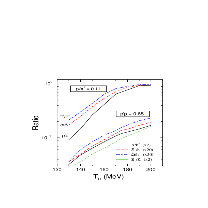
Figure 2: Dependence of particle yield ratios on Hagedorn temperature for a fireball characterized by the $B_{0}/m_{0}$ ratio adjusted to reproduce either the yield ratio of $p/\pi^{+}=0.11$ (upper set of lines) or $\overline{p}/p=0.65$ (lower set of lines). The ratios chosen for the adjustment represent the central Au+Au data at $\sqrt{s}=130A$ GeV.

In Fig. 2, we show the particle yield ratios that turn out to be particularly sensitive to the Hagedorn temperature under a given constraint. In one case, while varying the temperature, we adjust the initial fireball’s ratio $B_{0}/m_{0}$ to reproduce the ratio $\bar{p}/p\approx 0.65$ for the RHIC data (lower set of lines). In that case, the baryon-to-antibaryon ratios, $\bar{B}/B$, remain rather stable with $T_{H}$ variation; the strongest variations are observed for the ratio of strange baryons to the negatively charged hadrons or to the negative mesons. On the other hand, if we adjust the ratio $B_{0}/m_{0}$ to reproduce the ratio $p/\pi^{+}\approx 0.11$ (upper set of lines), strong variations are observed for the $\bar{B}/B$ ratios. No matter what fitting strategy is followed, a reasonable agreement with the data is obtained within the Hagedorn temperature range of $T_{H}=165-175\,\mbox{MeV}$.

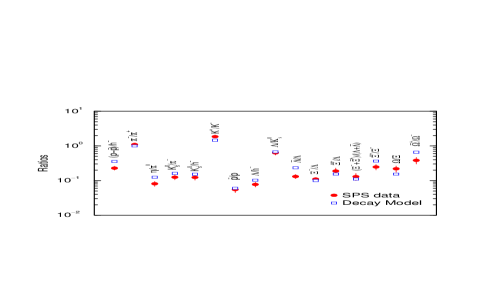
Figure 3: Particle yield ratios from the resonance decay model compared to the SPS Pb+Pb central-collision data at the laboratory energy of $158A$ GeV. In the model, at $T_{H}=170$ MeV, the starting baryon number of $B_{0}=26$ was assumed, in combination with the mass $m_{0}=100$ GeV and strangeness $S_{0}=0$.

We next confront our resonance decay model with the SPS abundance data from the central Pb+Pb collisions at the laboratory energy of $158A$ GeV. As illustrated in Fig. 3, an optimal agreement with the data is obtained for $m_{0}=100$ GeV when assuming (at $T_{H}=170$ MeV) a starting baryon number of $B_{0}=26$. While the general agreement is rather good, we note that the calculated ${\overline{\Omega}}^{+}/\Omega^{-}$ ratio is about $60\%$ larger than the data. It is likely that the assumption of a larger number of lighter initial resonances would improve the agreement; in the thermal model the discrepancy is tauted as strangeness undersaturation becattini .

Measured kinematic spectra of particles from central heavy ion collisions exhibit the effects of collective expansion. As may be expected, with suppressed fusion processes, our model produces kinematic spectra characterized by slope temperatures close to $T_{H}$ (see also Ref. moretto ). In the standard version of the model, the sequences of decay and fusion generate some collective motion, but not enough to explain the transverse RHIC spectra. For pions e.g. the slope temperature raises by 4% compared to the version without fusion. Moderate increases in the elastic cross section, such as to an overall 10 mb, raise kinematic temperatures further, 6% for pions, but not well enough to approach data. As a consequence, it is necessary to assume the presence of some collective motion early on in system evolution, leading to resonances that exhibit space-momentum correlations. It might be that the dynamics, beyond statistics, needs to be involved in the predominant decays, involving the interior degrees of freedom of resonances. The first resonances might also emerge at finite transverse velocities. In either case, degrees of freedom beyond resonances would be involved.

The transverse mass spectra displayed in Fig. 4 are obtained by folding a common collective velocity field with the spectra from our decay model. Specifically, we assume a uniform transverse velocity distribution, $d^{2}N/d\beta_{t}^{2}=\Theta(\beta_{t}-\beta_{\rm max})$. The spectra for all the hadrons can be best described, at $T_{H}=170$ MeV, with a uniform velocity field of $\beta_{\rm max}\approx 0.40$, corresponding to an average flow velocity of $\langle\beta_{t}\rangle=2\,\beta_{\rm max}/3\approx 0.27$. Notably, much less early flow, as characterized by $\langle\beta_{t}\rangle\approx 0.14$, is required to explain the particle spectra at SPS energy, see Fig. 5.

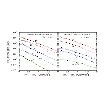
Figure 4: Transverse mass spectra of midrapidity hadrons at RHIC. Solid symbols are the data from PHENIX sppx (left panel) and STAR lblast ; mstrst (right panel) collaborations from central Au+Au collisions at the energy of $\sqrt{s}=130A$ GeV. The lines represent the model spectrum from convoluting the spectrum of the resonance decay model, at $T_{H}=170$ MeV, with a uniform transverse collective velocity distribution characterized by $\langle\beta_{t}\rangle=0.27$.

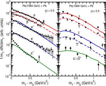
Figure 5: Transverse mass spectra of midrapidity hadrons at SPS. Solid symbols are the data from NA44 na44 (left panel) and WA97 wa97 collaborations from central Pb+Pb collisions at the energy of 158 AGeV. The lines represent the model spectrum from convoluting the spectrum of the resonance decay model, at $T_{H}=170$ MeV, with a uniform transverse collective velocity distribution characterized by $\langle\beta_{t}\rangle=0.14$.

In summary, we have formulated a statistical model of hadron resonance formation and decay. Within the model, the density of hadronic states in mass is described in terms of a universal Hagedorn-type temperature. We have demonstrated that both the RHIC and SPS abundance data can be suitably described in terms of resonance decays at the spectral temperature of $T_{H}\simeq 170$ MeV, even when pursuing the extreme assumption of a single heavy resonance populating the investigated rapidity region. To explain the data for particle spectra, we needed to invoke additional collective motion beyond that generated in the hadronic interactions.

- (1) Quark Matter 2004, Proc. of the 17th Int. Conf. on Ultra-Relativistic Nucleus-Nucleus Collisions, Oakland, USA; J. Phys. G 30 (2004).
- (2) M. Gyulassy and L. McLerran, Nucl. Phys. A 750 (2005) 30.
- (3) P. Braun-Munzinger, D. Magestro, K. Redlich and J. Stachel, Phys. Lett. B 518 (2001) 41.
- (4) K. Redlich, F. Karsch, and A. Tawfik, Phys. Lett. B 571 (2003) 67.
- (5) F. Becattini, M. Gaździcki, A. Keränen, J. Manninen and R. Stock, Phys. Rev. C 69 (2004) 024905.
- (6) P. Braun-Munzinger, J. Stachel, and C. Wetterich, Phys. Lett. B 596 (2004) 61.
- (7) F. Karsch, E. Laermann, and A. Peikert, Nucl. Phys. B 605 (2001) 579; F. Karsch and E. Laermann, hep-lat/0305025.
- (8) F. Becattini, A. Giovannini and S. Lupia, Z. Phys. C72 (1996) 491; F. Becattini, J. Phys. G23 (1997) 1933.
- (9) S. Bass, et al., Prog. Part. Nucl. Phys. 41 (1998) 225.
- (10) W. Cassing and E. Bratkovskaya, Phys. Rep. 308 (1999) 65.
- (11) Z. W. Lin, C. M. Ko, B.-A. Li, B. Zhang, and S. Pal, nucl-th/0411110.
- (12) A. J. Cole, Statistical Models for Nuclear Decay (Institute of Physics Publishing, Bristol, 2000).
- (13) R. Hagedorn, Suppl. Nuovo Cim. 3 (1965) 147.
- (14) W. Broniowski and W. Florkowski, Phys. Lett. B 490 (2000) 223.
- (15) P. Danielewicz and G. F. Bertsch, Nucl. Phys. A 533 (1991) 712.
- (16) E. Schnedermann, J. Sollfrank and U. Heinz, Phys. Rev. C 48 (1993) 2462.
- (17) As in the data, the results for ratios are corrected for feed down from weak decays, while the ratios involving particles with and include weak decays from heavier hyperons.
- (18) O. Barannikova and F. Wang, (for STAR Collaboration), Nucl. Phys. A 715 (2003) 458.
- (19) B. B. Back, et al., PHOBOS Collaboration, Phys. Rev. Lett. 87 (2001) 102301.
- (20) F. Videbaek, (for BRAHMS Collaboration), Nucl. Phys. A 698 (2002) 29; I. G. Bearden, (for BRAHMS Collaboration), Nucl. Phys. A 698 (2002) 667.
- (21) J. Adams, et al., STAR Collaboration, Phys. Lett. B 567 (2002) 167.
- (22) W. A. Zajc, (for PHENIX Collaboration), Nucl. Phys. A 698 (2002) 39.
- (23) C. Adler, et al., STAR Collaboration, Phys. Lett. B 595 (2004) 143.
- (24) C. Adler, et al., STAR Collaboration, Phys. Rev. Lett. 86 (2001) 4778., Erratum: Phys. Rev. Lett. 90 (2003) 119903(E).
- (25) I. G. Bearden, et al., BRAHMS Collaboration, Phys. Rev. Lett. 87 (2001) 112305.
- (26) J. Adcox, et al., PHENIX Collaboration, Phys. Rev. Lett. 89 (2002) 092302.
- (27) C. Adler, et al., STAR Collaboration, Phys. Rev. Lett. 89 (2002) 092301.
- (28) J. Adams, et al., STAR Collaboration, Phys. Rev. Lett. 92 (2004) 182301.
- (29) J. Castillo, (for STAR Collaboration), Nucl Phys. A 715 (2003) 518.
- (30) S. Pal, C. M. Ko and Z.-W. Lin, Nucl. Phys. A 730 (2004) 143.
- (31) C. Greiner and S. Leupold, J. Phys. G 27 (2001) L95; C. Greiner, P. Koch-Steinheimer, F. M. Liu, I. A. Shovkovy and H. Stöcker, hep-ph/0412095.
- (32) P. Koch, B. Müller and J. Rafelski, Phys. Rep. 142 (1986) 67.
- (33) L. G. Moretto, K. A. Bugaev, J. B. Elliot, L. G. Moretto and L. Phair, nucl-th/0412095; K. A. Bugaev, J. B. Elliot, L. G. Moretto and L. Phair, nucl-th/0504011.
- (34) K. Adcox, et al., PHENIX Collaboration, Phys. Rev. C 69 (2004) 024904.
- (35) I. G. Bearden, et al., NA44 Collaboration, Phys. Rev. Lett. 78 (1997) 2080.
- (36) F. Antinori, et al., WA97 Collaboration, Eur. Phys. J. C 14 (2000) 633.