CRITICAL LINE OF THE DECONFINEMENT PHASE TRANSITIONS

Abstract

Phase diagram of strongly interacting matter is discussed within the exactly solvable statistical model of the quark-gluon bags. The model predicts two phases of matter: the hadron gas at a low temperature $T$ and baryonic chemical potential $\mu_{B}$, and the quark-gluon gas at a high $T$ and/or $\mu_{B}$. The nature of the phase transition depends on a form of the bag mass-volume spectrum (its pre-exponential factor), which is expected to change with the $\mu_{B}/T$ ratio. It is therefore likely that the line of the 1^st order transition at a high $\mu_{B}/T$ ratio is followed by the line of the 2^nd order phase transition at an intermediate $\mu_{B}/T$, and then by the lines of ”higher order transitions” at a low $\mu_{B}/T$.

I Introduction

Investigation of the properties of strongly interacting matter at a high energy density is one of the most important subjects of the contemporary physics. In particular, the hypothesis that at high energy densities the matter is in the form of quark-gluon plasma (QGP) qgp rather than a gas of hadrons (HG) motivated a first stage of the broad experimental program of study of ultra-relativistic nucleus–nucleus collisions exp . Over the last 20 years rich data were collected by experiments located at Alternating Gradient Synchrotron (AGS) and Relativistic Heavy Ion Collider (RHIC) in Brookhaven National Laboratory, USA and at Super Proton Synchrotron (SPS) in CERN, Switzerland. The results indicate that the properties of the created matter change rapidly in the region of the low SPS energies onset ($\sqrt{s}_{NN}\approx$ 6–12 GeV). The observed effects confirm predictions for the transition from hadron gas to QGP gago and thus indicate that in fact a new form of strongly interacting matter exists in nature at sufficiently high energy densities.

What are the properties of the transition between the two phases of strongly interacting matter? This question motivates the second stage of the investigation of nucleus-nucleus collisions. A new experimental heavy ion program ($\sqrt{s}_{NN}\approx$ 5–20 GeV) at the CERN SPS is in preparation loi and a possible study at the BNL RHIC is under discussion.

Based on the numerous examples of the well-known substances a conjecture was formulated (see review paper misha and references there in) that the transition from HG to QGP is a 1^st order phase transition at low values of a temperature $T$ and a high baryo-chemical potential $\mu_{B}$ and it is a rapid cross–over at a high $T$ and a low $\mu_{B}$. The end point of the 1^st order phase transition line is expected to be the 2^nd order critical point. This hypothesis seems to be supported by QCD–based qualitative considerations misha and first semi–quantitative lattice QCD calculations fodorkatz . The properties of the deconfinement phase transition are, however, far from being well established. This stimulates our study of the transition domain within the statistical model of quark-gluon bags.

The bag model bag was invented in order to describe the hadron spectrum, the hadron masses and their proper volumes. This model is also successfully used for a description of the deconfined phase (see e.g. Ref. bag-qgp ). Thus the model suggests a possibility for a unified treatment of both phases. Any configuration of the system and, therefore, each term in the system partition function, can be regarded as a many-bag state both below and above the transition domain. The statistical model of quark-gluon bags discussed in this paper contains in itself two well-known models of deconfined and confined phases: the bag model of the QGP bag-qgp and the hadron gas models hg . They are surprisingly successful in describing the bulk properties of hadron production in high energy nuclear collisions and thus one may hope that the model presented here may reflect the basic features of nature in the transition domain.

The paper is organized as follows. The important properties of the statistical bootstrap model with the van der Waals repulsion are summarized in Sect. II. In Sect. III the statistical model of the quark–gluon bags is presented. Within this model properties of the transition region for $\mu_{B}=0$ are studied in Sect. IV and the analysis is extended to the complete $T-\mu_{B}$ plane in Sect. V. The paper is closed by the summary and outlook given in Sect. VI.

II Statistical Bootstrap Model and Van der Waals Repulsion

The grand canonical partition function for an ideal Boltzmann gas of particles of mass $m$ and a number of internal degrees of freedom (a degeneracy factor) $g$, in a volume $V$ and at a temperature $T$ is given by:

$$Z(V,T)~{}=~{}\sum_{N=0}^{\infty}~{}\frac{1}{N!}~{}\prod_{j=1}^{N}\int\frac{gV\;d^{3}k_{j}}{(2\pi)^{3}}\exp\left[~{}-~{}\frac{(k_{j}^{2}~{}+~{}m^{2})^{1/2}}{T}~{}\right]~{}=~{}\sum_{N=0}^{\infty}\frac{[V~{}g\phi(T,m)]^{N}}{N!}~{}=~{}\exp[Vg\phi(T,m)]~{},$$ (1)

where

$$\phi(T,m)~{}\equiv~{}\frac{1}{2\pi^{2}}~{}\int_{0}^{\infty}k^{2}dk~{}\exp\left[-~{}\frac{(k^{2}~{}+~{}m^{2})^{1/2}}{T}\right]~{}=~{}\frac{m^{2}T}{2\pi^{2}}~{}K_{2}\left(\frac{m}{T}\right)$$ (2)

and $K_{2}$ is the modified Bessel function. The function $\phi(T,m)$ is equal to the particle number density:

$$n(T)~{}\equiv~{}\frac{\overline{N}(V,T)}{V}~{}=~{}g\phi(T,m)~{}.$$ (3)

The ideal gas pressure and energy density can be derived from Eq. (1) as:

$$p(T)~{}\equiv~{}T~{}\frac{\ln Z(V,T)}{V}~{}=~{}T~{}g\phi(T,m)~{},~{}~{}~{}~{}\varepsilon(T)~{}\equiv~{}T~{}\frac{dp}{dT}~{}-~{}p(T)~{}=~{}T^{2}~{}g\frac{d\phi(T,m)}{dT}~{}.$$ (4)

One can easily generalize the ideal gas formulation (1) to the mixture of particles with masses $m_{1},...,m_{n}$ and degeneracy factors $g_{1},...,g_{n}$:

$$Z(V,T)~{}=~{}\sum_{N_{1}=0}^{\infty}~{}...~{}\sum_{N_{n}=0}^{\infty}\frac{\left[Vg_{1}\phi(T,m_{1})\right]^{N_{1}}}{N_{1}!}~{}...~{}\frac{\left[Vg_{n}\phi(T,m_{n})\right]^{N_{n}}}{N_{n}!}~{}=~{}\exp\left[V~{}\sum_{j=1}^{n}g_{j}\phi(T,m_{j})\right]~{}.$$ (5)

The sum over different particle species $j$ can be extended to infinity. It is convenient to introduce the mass spectrum density $\rho(m)$, so that $\rho(m)dm$ gives the number of different particle mass states in the interval $[m,m+dm]$, i.e. $\sum_{j=1}^{\infty}g_{j}...=\int_{0}^{\infty}dm...\rho(m)$. In this case the pressure and the energy density are given by:

$$p(T)~{}=~{}T~{}\int_{0}^{\infty}dm~{}\rho(m)~{}\phi(T,m)~{},~{}~{}~{}~{}\varepsilon(T)~{}=~{}T^{2}~{}\int_{0}^{\infty}dm~{}\rho(m)~{}\frac{d\phi(T,m)}{dT}~{}.$$ (6)

Eqs. (6) were introduced by Hagedorn Hag for the mass spectrum increasing exponentially for $m\rightarrow\infty$:

$$\rho(m)\simeq~{}C~{}m^{-a}~{}\exp(bm)~{},$$ (7)

where $a$, $b$ and $C$ are model parameters. This form of the spectrum (7) was further derived from the statistical bootstrap model Frau . It can be shown, that within this model the temperature $T_{H}\equiv 1/b$ (the ”Hagedorn temperature”) is the maximum temperature of the matter. The behavior of thermodynamical functions (6) with the mass spectrum (7) depends crucially on the parameter $a$. In particular, in the limit $T\rightarrow T_{H}$ the pressure and the energy density approach:

$$p~{},~{}\varepsilon~{}\rightarrow~{}\infty~{},~{}~{}~{}~{}~{}~{}~{}~{}~{}~{}~{}~{}~{}~{}~{}~{}~{}~{}~{}~{}~{}{\rm for}~{}~{}~{}a~{}\leq~{}\frac{5}{2}~{};$$ (8)

$$p~{}\rightarrow const~{},~{}\varepsilon~{}\rightarrow~{}\infty~{},~{}~{}~{}~{}~{}~{}~{}~{}{\rm for}~{}~{}~{}\frac{5}{2}~{}\leq~{}a~{}\leq~{}\frac{7}{2}~{};$$ (9)

$$p~{},~{}\varepsilon~{}\rightarrow~{}const~{},~{}~{}~{}~{}~{}~{}~{}~{}~{}~{}~{}~{}~{}~{}~{}~{}~{}{\rm for}~{}~{}~{}a~{}>~{}\frac{7}{2}~{}.$$ (10)

Up to here all particles including those with $m\rightarrow\infty$ were treated as point-like objects. Clearly this is an unrealistic feature of the statistical bootstrap model. It can be overcome by introduction of hadron proper volumes which simultaneously mimic the repulsive interactions between hadrons. The van der Waals excluded volume procedure pt can be applied for this purpose pt (other approaches were discussed in Refs. HR ; K ). The volume $V$ of the ideal gas (1) is substituted by the ”available volume” $V-v_{o}N$, where $v_{o}$ is a parameter which corresponds to a particle proper volume. The partition function then reads:

$$Z(V,T)~{}=~{}\sum_{N=0}^{\infty}\frac{[(V~{}-~{}v_{o}N)~{}g\phi(T,m)]^{N}}{N!}~{}\theta(V-v_{o}N)~{}.$$ (11)

The pressure of the van der Waals gas can be calculated from the partition function (11) by use of its Laplace transform. This procedure is necessary because the ”available volume”, $V-v_{o}N$, depends on the particle number $N$. The Laplace transform of (11) is pt ; vdw1 :

$$\hat{Z}(s,T)~{}\equiv\int_{0}^{\infty}dV\exp(-sV)~{}Z(V,T)~{}=~{}\sum_{N=0}^{\infty}\frac{[g\phi(T,m)]^{N}}{N!}\int_{v_{o}N}^{\infty}dV~{}(V~{}-~{}v_{o}N)^{N}~{}\exp(-sV)$$

$$=~{}\frac{1}{s}~{}\sum_{N=0}^{\infty}\left[\frac{\exp(-v_{o}s)~{}g\phi(T,m)}{s}\right]^{N}~{}=~{}\left[~{}s~{}-~{}\exp(-v_{o}s)~{}g\phi(T,m)\right]^{-1}~{}.$$ (12)

In the thermodynamic limit, $V\rightarrow\infty$, the partition function behaves as $Z(V,T)\simeq\exp\left[pV/T\right]$. An exponentially increasing $Z(V,T)$ generates the farthest-right singularity $s^{*}=p/T$ of the function $\hat{Z}(s,T)$ in variable $s$. This is because the integral over $V$ in Eq. (II) diverges at its upper limit for $s<p/T$. Consequently, the pressure can be expressed as

$$p(T)~{}=~{}T~{}\lim_{V\rightarrow\infty}\frac{\ln Z(V,T)}{V}~{}=~{}T~{}s^{*}(T)~{},$$ (13)

and the farthest-right singularity $s^{*}$ of $\hat{Z}(s,T)$ (II) can be calculated from the transcendental equation pt ; vdw1 :

$$s^{*}(T)~{}=~{}\exp\left[-~{}v_{o}s^{*}(T)\right]~{}g\phi(T,m)~{}.$$ (14)

Note that the singularity $s^{*}$ is not related to phase transitions in the system. Such a singularity exists for any statistical system. For example, for the ideal gas ($v_{o}=0$ in Eq. (14)) $s^{*}=g\phi(T,m)$ and thus from Eq. (13) one gets $p=Tg\phi(T,m)$ which corresponds to the ideal gas equation of state (4).

III Gas of Quark-Gluon Bags

The van der Waals gas consisting of $n$ hadronic species, which are called bags in what follows. is considered in this section. Its partition function reads:

$$Z(V,T)~{} =~{}\sum_{N_{1}=0}^{\infty}~{}...~{}\sum_{N_{n}=0}^{\infty}\frac{\left[\left(V-v_{1}N_{1}-...-v_{n}N_{n}\right)~{}g_{1}\phi(T,m_{1})\right]^{N_{1}}}{N_{1}!}~{}\times...$$

$$...~{}\times~{}\frac{\left[\left(V-v_{1}N_{1}-...-v_{n}N_{n}\right)~{}g_{n}\phi(T,m_{n})\right]^{N_{n}}}{N_{n}!}~{}\theta\left(V-v_{1}N_{1}-...-v_{n}N_{n}\right)~{},$$ (15)

where $(m_{1},v_{1}),...,(m_{n},v_{n})$ are the masses and volumes of the bags. The Laplace transformation of Eq. (15) gives

$$\hat{Z}(s,T)~{}=~{}\left[~{}s~{}-~{}\sum_{j=1}^{n}\exp\left(-v_{j}s\right)~{}g_{j}\phi(T,m_{j})\right]^{-1}~{}.$$ (16)

As long as the number of bags, $n$, is finite, the only possible singularity of $\hat{Z}(s,T)$ (16) is its pole. However, in the case of an infinite number of bags the second singularity of $\hat{Z}(s,T)$ may appear. This case is discussed in what follows.

Introducing the bag mass-volume spectrum, $\rho(m,v)$, so that $\rho(m,v)dmdv$ gives the number of bag states in the mass-volume interval $[m,v;m+dm,v+dv]$, the sum over different bag states in definition of $Z(V,T)$ can be replaced by the integral, $\sum_{j=1}^{\infty}g_{j}...=\int_{0}^{\infty}dmdv...\rho(m,v)$. Then, the Laplace transform of $Z(V,T)$ reads pt :

$$\hat{Z}(s,T)~{} \equiv\int_{0}^{\infty}dV\exp(-sV)~{}Z(V,T)~{}=~{}\left[~{}s~{}-~{}f(T,s)\right]^{-1}~{},$$ (17)

where

$$f(T,s)~{} =~{}\int_{0}^{\infty}dmdv~{}\rho(m,v)~{}\exp(-vs)~{}\phi(T,m)~{}.$$ (18)

The pressure is again given by the farthest-right singularity: $p(T)=Ts^{*}(T)$. One evident singular point of $\hat{Z}(s,T)$ (17) is the pole singularity, $s_{H}(T)$:

$$s_{H}(T)~{}=~{}f\left(T,s_{H}(T)\right)~{}.$$ (19)

As mentioned above this is the only singularity of $\hat{Z}(s,T)$ if one restricts the mass-volume bag spectrum to a finite number of states. For an infinite number of mass-volume states the second singular point of $\hat{Z}(s,T)$ (17), $s_{Q}(T)$, can emerge, which is due to a possible singularity of the function $f(T,s)$ (18) itself. The system pressure takes then the form:

$$p(T)~{}=~{}Ts^{*}(T)~{}=~{}T\cdot max\{s_{H}(T),s_{Q}(T)\}~{},$$ (20)

and thus the farthest-right singularity $s^{*}(T)$ of $\hat{Z}(s,T)$ (17) can be either the pole singularity $s_{H}(T)$ (19) or the $s_{Q}(T)$ singularity of the function $f(T,s)$ (18) itself. The mathematical mechanism for possible phase transition (PT) in our model is the ”collision” of the two singularities, i.e. $s_{H}(T)=s_{Q}(T)$ at PT temperature $T=T_{C}$ (see Fig. 1) . In physical terms this can be interpreted as the existence of two phases of matter, namely, the hadron gas with the pressure, $p_{H}=Ts_{H}(T)$, and the quark gluon plasma with the pressure $p_{Q}=Ts_{Q}(T)$. At a given temperature $T$ the system prefers to stay in a phase with the higher pressure. The pressures of both phases are equal at the PT temperature $T_{C}$.

An important feature of this modeling of the phase transition should be stressed here. The transition, and thus the occurrence of the two phases of matter, appears as a direct consequence of the postulated general partition function (a single equation of state). Further on, the properties of the transition, e.g. its location and order, follow from the partition function and are not assumed. This can be confronted with the well-known phenomenological construction of the phase transition, in which the existence of the two different phases of matter and the nature of the transition between them are postulated.

The crucial ingredient of the model presented here which defines the presence, location and the order of the PT is the form of the mass-volume spectrum of bags $\rho(m,v)$. In the region where both $m$ and $v$ are large it can be described within the bag model bag . In the simplest case of a bag filled with the non-interacting massless quarks and gluons one finds pt1 :

$$\rho(m,v)~{}\simeq~{}C~{}v^{\gamma}(m-Bv)^{\delta}~{}\exp\left[\frac{4}{3}~{}\sigma_{Q}^{1/4}~{}v^{1/4}~{}(m-Bv)^{3/4}\right]~{},$$ (21)

where $C$, $\gamma$, $\delta$ and $B$ (the so-called bag constant, $B\approx 400$ MeV/fm³ bag-qgp ) are the model parameters and

$$\sigma_{Q}~{}=~{}\frac{\pi^{2}}{30}\left(g_{g}~{}+~{}\frac{7}{8}g_{q\bar{q}}\right)~{}=~{}\frac{\pi^{2}}{30}\left(2\cdot 8~{}+~{}\frac{7}{8}\cdot 2\cdot 2\cdot 3\cdot 3\right)~{}=~{}\frac{\pi^{2}}{30}~{}\frac{95}{2}$$ (22)

is the Stefan-Boltzmann constant counting gluons (spin, color) and (anti-)quarks (spin, color and $u$, $d$, $s$-flavor) degrees of freedom. This is the asymptotic expression assumed to be valid for a sufficiently large volume and mass of a bag, $v>V_{0}$ and $m>Bv+M_{0}$. The validity limits can be estimated to be $V_{0}\approx 1$ fm³ and $M_{0}\approx 2$ GeV pt2 . The mass-volume spectrum function:

$$\rho_{H}(m,v)~{}=~{}\sum_{j=1}^{n}~{}g_{j}~{}\delta(m-m_{j})~{}\delta(v-v_{j})$$ (23)

should be added to $\rho(m,v)$ in order to reproduce the known low-lying hadron states located at $v<V_{0}$ and $m<BV_{0}+M_{0}$. The mass spectra of the resonances are described by the Breit-Wigner functions. Consequently, a general form of $f(T,s)$ (18) reads:

$$f(T,s)~{}\equiv~{}f_{H}(T,s)+f_{Q}(T,s)=\sum_{j=1}^{n}g_{j}\exp(-v_{j}s)~{}\phi(T,m_{j})+\int_{V_{o}}^{\infty}dv\int_{M_{o}+Bv}^{\infty}dm~{}\rho(m,v)\exp(-sv)\phi(T,m)~{},$$ (24)

where $\rho(m,v)$ is given by Eq. (21).

The behavior of $f_{Q}(T,s)$ is discussed in the following. The integral over mass in Eq. (24) can be calculated by the steepest decent estimate. Using the asymptotic expansion of the $K_{2}$-function one finds $\phi(T,m)\simeq(mT/2\pi)^{3/2}\exp(-m/T)$ for $m\gg T$. A factor exponential in $m$ in the last term of Eq. (24) is given by:

$$\exp\left[-\frac{m}{T}~{}+~{}\frac{4}{3}\sigma_{Q}^{1/4}v^{1/4}(m-Bv)^{3/4}\right]~{}\equiv~{}\exp[U(m)]~{}.$$ (25)

The function $U(m)$ has a maximum at:

$$m_{0}~{}=~{}\sigma_{Q}T^{4}v~{}+~{}Bv~{}.$$ (26)

Presenting $U(m)$ as

$$U(m)~{}\simeq~{}U(m_{0})~{}+~{}\frac{1}{2}~{}\left(\frac{d^{2}U}{dm^{2}}\right)_{m=m_{0}}~{}(m-m_{0})^{2}~{}=~{}vs_{Q}(T)~{}-~{}\frac{(m-m_{0})^{2}}{8\sigma_{Q}~{}vT^{5}}~{},$$ (27)

with

$$s_{Q}(T)~{}\equiv~{}\frac{1}{3}~{}\sigma_{Q}~{}T^{3}~{}-~{}\frac{B}{T}~{},$$ (28)

one finds

$$f_{Q}(T,s)~{}\simeq~{}u(T)~{}\int_{V_{0}}^{\infty}dv~{}v^{2+\gamma+\delta}~{}\exp\left[-v\left(s~{}-s_{Q}(T)\right)\right]~{},$$ (29)

where $u(T)=C\pi^{-1}\sigma_{Q}^{\delta+1/2}~{}T^{4+4\delta}~{}\left(\sigma_{Q}T^{4}+B\right)^{3/2}$. The function $f_{Q}(T,s)$ (29) has the singular point $s=s_{Q}$ because for $s<s_{Q}$ the integral over $dv$ diverges at its upper limit.

The first term of Eq. (24), $f_{H}$, represents the contribution of a finite number of low-lying hadron states. This function has no $s$-singularities at any temperature $T$. The integration over the region $m,v\rightarrow\infty$ generates the singularity $s_{Q}(T)$ (28) of the $f_{Q}(T,s)$ function (29). As follows from the discussion below this singularity should be associated with the QGP phase.

By construction the function $f(T,s)$ (18) is a positive one, so that $s_{H}(T)$ (19) is also positive. On the other hand, it can be seen from Eq. (28) that at a low $T$ $s_{Q}(T)<0$. Therefore, $s_{H}>s_{Q}$ at small $T$, and according to Eq. (20) it follows:

$$p(T)~{}=~{}T~{}s_{H}~{},~{}~{}~{}~{}\varepsilon(T)~{}=~{}T^{2}~{}\frac{ds_{H}}{dT}~{}.$$ (30)

The system of the quark-gluon bags is in a hadron phase.

If two singularities ”collide”, $T=T_{C}$ and $s_{H}(T_{C})=s_{Q}(T_{C})$, the singularity $s_{Q}(T)$ can become the farthest-right singularity at $T>T_{C}$. In Fig. 1 the dependence of the function $f(T,s)$ on $s$ and its singularities are sketched for $T_{1}<T_{2}=T_{C}<T_{3}$. The thermodynamical functions defined by the singularity $s_{Q}(T)$ are:

$$p(T)~{}=~{}T~{}s_{Q}~{}=~{}\frac{\sigma_{Q}}{3}~{}T^{4}~{}-~{}B~{},~{}~{}~{}~{}\varepsilon(T)~{}=~{}T^{2}~{}\frac{ds_{Q}}{dT}~{}=~{}\sigma_{Q}~{}T^{4}~{}+~{}B~{}$$ (31)

and thus they describe the QGP phase.

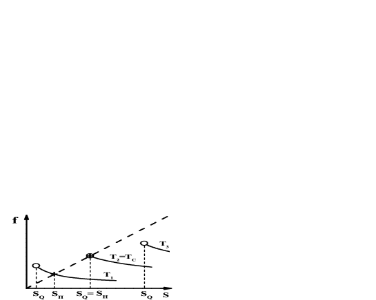
Figure 1: The dependence of $f(T,s)$ on $s$ for three different temperatures: $T_{1}<T_{2}=T_{C}<T_{3}$ (solid lines). The pole singularity $s_{H}$ and the singularity $s_{Q}$ are denoted by circles and crosses, respectively. A PT corresponds to the ”collision” of two singularities $s_{H}=s_{Q}$ at the temperature $T_{C}$.

The existence and the order of the phase transition depend on the values of the parameters of the model. From Eq. (29) follows that a PT exists, i.e. $s^{*}=s_{Q}$ at high $T$, provided $\gamma+\delta<-3$ (otherwise $f(T,s_{Q})=\infty$, and $s_{H}>s_{Q}$ for all $T$, for illustration see Fig. 2, left).

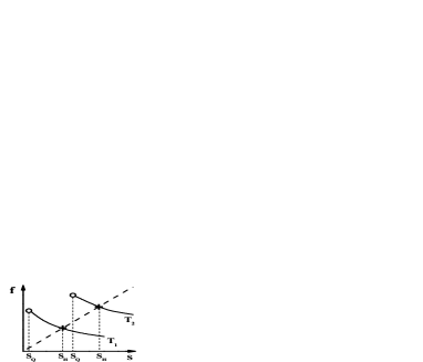
Figure 2: The dependence of $f(T,s)$ on $s$ for two different temperatures, $T_{1}<T_{2}$ (solid lines). The figures demonstrate the absence of the PT in the model if $f(T,s_{Q})=\infty$ (left), or if $f(T,s_{Q})>s_{Q}$ at all $T$ (right).

In addition it is required that $f(T,s_{Q})<s_{Q}(T)$ at $T\rightarrow\infty$, (otherwise $s^{*}=s_{H}>s_{Q}$ for all $T$, for illustration see Fig. 2, right). For $\gamma+\delta<-3$ one finds $f_{Q}(T,s_{Q})\propto T^{10+4\delta}$ at $T\rightarrow\infty$. On the other hand, $s_{Q}(T)\propto T^{3}$ at a high $T$ and therefore $\delta<-7/4$. Consequently the general conditions for the existence of any phase transition in the model are:

$$\gamma~{}<~{}-~{}\frac{5}{4}~{},~{}~{}~{}~{}~{}~{}~{}\delta~{}<~{}-~{}\frac{7}{4}~{}.$$ (32)

The parameters $\gamma$ and $\delta$ can be calculated within the model provided constraints defining allowed quark-gluon bags are given pt1 ; pt2 . Assuming massless non-interacting quarks and gluons with the condition of the total three-momentum vector equal to zero one gets pt1 :

$$\gamma~{}=~{}-~{}\frac{5}{4}~{},~{}~{}~{}~{}~{}~{}~{}\delta~{}=~{}-~{}\frac{7}{4}~{},$$ (33)

and consequently there is no phase transition in the model. For a graphical illustration of this case see Fig. 2 left. An additional selection of only colorless bags yields pt2 :

$$\gamma~{}=~{}-~{}\frac{9}{4}~{},~{}~{}~{}~{}~{}~{}~{}\delta~{}=~{}-~{}\frac{19}{4}~{},$$ (34)

so that the conditions (32) are fulfilled and the model leads to the phase transition, see Fig. 1 for illustration. Based on these two simple examples one concludes that the parameters $\gamma$ and $\delta$ depend significantly on the set of selected constraints. These constraints in statistical mechanics are usually ignored as the related to them pre-exponential factors do not contribute to the equation of state in the thermodynamic limit. Because of this possible sets of physical constraints are not well defined and their consequences were not studied. Therefore in what follows $\gamma$ and $\delta$ are considered as free model parameters.

IV 1^st, 2^nd and higher ORDER PHASE TRANSITIONS

In this section the order of the PT in the system of quark-gluon bags is discussed.

The 1^st order PT takes place at $T=T_{C}$ provided:

$$s_{Q}(T_{C})~{}=~{}s_{H}(T_{C})~{},~{}~{}~{}~{}\left(\frac{ds_{Q}}{dT}\right)_{T=T_{C}}~{}>~{}\left(\frac{ds_{H}}{dT}\right)_{T=T_{C}}~{}.$$ (35)

Thus the energy density ($\varepsilon=T^{2}ds/dT$) has discontinuity (latent heat) at the 1^st order PT. Its dependence on $T$ is shown in Fig. 3, left. In calculating $ds_{H}/dT$ it is important to note that the function $s_{H}(T)$ (19) is only defined for $T\leq T_{C}$, i.e. for $s_{H}(T)\geq s_{Q}(T)$.

Figure 3: The dependence of the energy density $\varepsilon$ on temperature for the 1^st (left) and 2^nd (right) order PT. The energy density $\varepsilon(T)$ has a discontinuity at $T=T_{C}$ for the 1^st order PT whereas for the 2^nd order PT $\varepsilon(T)$ is a continuous function of $T$, but $d\varepsilon/dT$ has a discontinuity at $T=T_{C}$.

The 2^nd order PT takes place at $T=T_{C}$ provided:

$$s_{Q}(T_{C})~{}=~{}s_{H}(T_{C})~{},~{}~{}~{}~{}\left(\frac{ds_{Q}}{dT}\right)_{T=T_{C}}~{}=~{}\left(\frac{ds_{H}}{dT}\right)_{T=T_{C}}~{},~{}~{}~{}~{}\left(\frac{d^{2}s_{H}}{d^{2}T}\right)_{T=T_{C}}~{}\neq~{}\left(\frac{d^{2}s_{Q}}{d^{2}T}\right)_{T=T_{C}}~{}.$$ (36)

Hence the energy density is a continuous function of $T$, but its first derivate has a discontinuity, for illustration see Fig. 3, right.

What is the order of the PT in the model? To answer this question Eq. (19) should be rewritten as:

$$s_{H}~{}=~{}f_{H}~{}+~{}u~{}\int_{V_{o}}^{\infty}dvv^{-\alpha}\exp\left[-v\left(s_{H}-s_{Q}\right)\right]~{},$$ (37)

where $\alpha\equiv-(\gamma+\delta+2)~{}>1$. Differentiating both sides with respect to $T$ (the prime denotes the $d/dT$ derivative) one gets:

$$s_{H}^{\prime}~{}=~{}f_{H}^{\prime}~{}+~{}u^{\prime}~{}\int_{V_{o}}^{\infty}dvv^{-\alpha}~{}\exp\left[-v\left(s_{H}-s_{Q}\right)\right]~{}+u~{}\int_{V_{o}}^{\infty}dvv^{-\alpha+1}~{}\left(s_{Q}^{\prime}-s_{H}^{\prime}\right)~{}\exp\left[-v\left(s_{H}-s_{Q}\right)\right]~{},$$ (38)

from which follows:

$$s_{H}^{\prime}~{}=~{}\frac{G~{}+~{}F\cdot s_{Q}^{\prime}}{1~{}+~{}F}~{},$$ (39)

where

$$G~{}\equiv~{}f_{H}^{\prime}+u^{\prime}\int_{V_{o}}^{\infty}dvv^{-\alpha}\exp\left[-v\left(s_{H}-s_{Q}\right)\right]~{},~{}~{}~{}~{}F~{}\equiv~{}u~{}\int_{V_{o}}^{\infty}dvv^{-\alpha+1}\exp\left[-v\left(s_{H}-s_{Q}\right)\right]~{}.$$ (40)

It is easy to see that the transition is of the 1^st order, i.e. $s_{Q}^{\prime}(T_{C})>s_{H}^{\prime}(T_{C})$, provided $\alpha>2$. The 2^nd or higher order phase transition takes place provided $s_{Q}^{\prime}(T_{C})=s_{H}^{\prime}(T_{C})$ at $T=T_{C}$. This condition is satisfied when $F(T)$ diverges to infinity at $T\rightarrow(T_{C}-0)$, i.e. for $T$ approaching $T_{C}$ from below.

One notes that the exponential factor in $\rho(m,v)$ (21) generates the singularity $s_{Q}(T)$ (28) of the $\hat{Z}(s,T)$ function (17). Due to this there is a possibility of a phase transition in the model. Whether it does exist and what the order is depends on the values of the parameters $\gamma$ and $\delta$ in the pre-exponential power-like factor, $v^{\gamma}(m-Bv)^{\delta}$, of the mass-volume bag spectrum $\rho(m,v)$ (21). This resembles the case of the statistical bootstrap model discussed in Sec. II. The limiting temperature $T_{H}=1/b$ appears because of the exponentially increasing factor $\exp(bm)$, in the mass spectrum (7), but the thermodynamical behavior (8-10) at $T=T_{H}$ depends crucially on the value of the parameter $a$ in the pre-exponential factor, $m^{-a}$ (7).

What is the physical difference between $\alpha>2$ and $1<\alpha\leq 2$ in the model? From Eq. (37) it follows that the volume distribution function of quark-gluon bags at $T<T_{C}$ has the form

$$W(v)~{}\propto~{}v^{-\alpha}~{}\exp\left[-v\left(s_{H}-s_{Q}\right)\right]~{}.$$ (41)

Consequently the average bag volume:

$$\overline{v}~{}=~{}\int_{V_{o}}^{\infty}dv~{}v~{}W(v)~{},$$ (42)

at $T~{}\rightarrow~{}(T_{Q}-0)$ approaches:

$$\overline{v}~{}=~{}const~{},~{}~{}~{}~{}~{}~{}~{}~{}{\rm for}~{}~{}~{}~{}\alpha~{}>~{}2~{};$$ (43)

$$\overline{v}~{}\rightarrow~{}\infty~{},~{}~{}~{}~{}~{}~{}~{}~{}~{}~{}~{}{\rm for}~{}~{}~{}~{}1~{}<~{}\alpha~{}\leq~{}2~{}.$$ (44)

Thus in the vicinity of the 1^st order PT the finite volume bags (”hadrons”) dominate at $T<T_{C}$. There is a single infinite volume bag (QGP) at $T>T_{C}$ and a mixed phase at $T=T_{C}$ (see also Ref. pt3 ). For the 2^nd order and/or ”higher order transitions” the dominant bag configurations include the large volume bags already in a hadron phase $T<T_{C}$, and the average bag volume increases to infinity at $T\rightarrow(T_{C}-0)$.

The condition for the 2^nd order PT can be derived as following. The integral for the function $F$ in Eq. (40) reads

$$\int_{V_{o}}^{\infty}dvv^{-\alpha+1}\exp\left[-v\left(s_{H}-s_{Q}\right)\right]~{}=~{}\left(s_{H}-s_{Q}\right)^{-2+\alpha}~{}\Gamma\left[2-\alpha,(s_{H}-s_{Q})V_{o}\right]~{},$$ (45)

where $\Gamma(k,x)$ is the incomplete Gamma-function. Thus using Eq. (39) one finds at $T\rightarrow(T_{C}-0)$:

$$s_{Q}^{\prime}~{}-~{}s_{H}^{\prime}~{} \propto~{}\left(s_{H}~{}-~{}s_{Q}\right)^{2-\alpha}~{},~{}~{}~{}~{}~{}~{}~{}~{}~{}~{}~{}~{}~{}{\rm for}~{}~{}~{}~{}~{}\alpha~{}<~{}2~{},$$ (46)

$$s_{Q}^{\prime}~{}-~{}s_{H}^{\prime}~{} \propto~{}-~{}\ln^{-1}\left(s_{H}~{}-~{}s_{Q}\right)~{},~{}~{}~{}~{}~{}~{}~{}~{}{\rm for}~{}~{}~{}~{}~{}\alpha~{}=~{}2~{},$$ (47)

and consequently:

$$s_{H}^{\prime\prime}~{}-s_{Q}^{\prime\prime}~{} \propto~{}(s_{H}~{}-~{}s_{Q})^{3-2\alpha}~{}~{}~{}~{}~{}~{}~{}~{}~{}{\rm for}~{}~{}~{}~{}~{}~{}~{}~{}~{}\alpha~{}<~{}2~{};$$ (48)

$$s_{H}^{\prime\prime}~{}-s_{Q}^{\prime\prime}~{} \propto~{}-~{}\frac{\ln^{-3}(s_{H}-s_{Q})}{s_{H}~{}-~{}s_{Q}}~{}~{}~{}~{}~{}~{}~{}{\rm for}~{}~{}~{}~{}~{}~{}~{}~{}~{}\alpha~{}=~{}2~{}.$$ (49)

Therefore for $3/2<\alpha\leq 2$ the 2^nd order PT with $s_{H}^{\prime\prime}(T_{C})=\infty$ takes place whereas for $\alpha=3/2$ the 2^nd order PT with the finite value of $s_{H}^{\prime\prime}(T_{C})$ is observed. The dependence of the specific heat $C\equiv d\varepsilon/dT$ on $T$ is shown in Fig. 4, left.

Figure 4: The dependence of the specific heat on temperature for the 2^nd order PT (left) and for the $3^{rd}$ order PT (right). Large values of $C$ in the hadron phase reflect the fact that large derivative $d\varepsilon_{H}/dT$ at $T$ close to $T_{C}$ is needed for the 2^nd and $3^{rd}$ order PT to reach the value of $\varepsilon_{Q}(T_{C})$ without energy density discontinuity.

An infinite value of a specific heat $C$ at $T\rightarrow(T_{C}-0)$ obtained within the model for $3/2<\alpha\leq 2$ is typical for the 2^nd order PTs LL .

From Eq. (48) it follows that $s_{H}^{\prime\prime}(T_{C})=s_{Q}^{\prime\prime}(T_{C})$ for $\alpha<3/2$. Using Eqs. (46, 48) one finds at $T\rightarrow(T_{C}-0)$:

$$s_{H}^{\prime\prime\prime}~{}-~{}s_{Q}^{\prime\prime\prime}~{}\propto~{}(s_{H}~{}-~{}s_{Q})^{4-3\alpha}~{}.$$ (50)

Thus, for $4/3\leq\alpha<3/2$ there is a $3^{rd}$ order transition:

$$s_{H}(T_{C})~{}=~{}s_{Q}(T_{C})~{},~{}~{}~{}~{}s_{H}^{\prime}(T_{C})~{}=~{}s_{Q}^{\prime}(T_{C})~{},~{}~{}~{}~{}s_{H}^{\prime\prime}(T_{C})~{}=~{}s_{Q}^{\prime\prime}(T_{C})~{},~{}~{}~{}~{}s_{H}^{\prime\prime\prime}(T_{C})~{}\neq~{}s_{Q}^{\prime\prime\prime}(T_{C})~{},$$ (51)

with $s_{H}^{\prime\prime\prime}(T_{C})=\infty$ for $4/3<\alpha<3/2$ and with a finite value of $s_{H}^{\prime\prime\prime}(T_{C})$ for $\alpha=4/3$. The dependence of the specific heat $C\equiv d\varepsilon/dT$ on temperature for the $3^{rd}$ order transition is shown in Fig. 4, right.

By calculating higher order derivatives of $s_{H}$ and $s_{Q}$ with respect to $T$ it can be shown that for $(n+1)/n\leq\alpha<n/(n-1)$ ($n=4,5,...$) there is a $n^{th}$ order transition

$$s_{H}(T_{C})~{}=~{}s_{Q}(T_{C})~{},~{}~{}~{}~{}s_{H}^{\prime}(T_{C})~{}=~{}s_{Q}^{\prime}(T_{C})~{},~{}~{}~{}~{}...~{}~{}~{}s_{H}^{(n-1)}(T_{C})~{}=~{}s_{Q}^{(n-1)}(T_{C})~{},~{}~{}~{}~{}s_{H}^{(n)}(T_{C})~{}\neq~{}s_{Q}^{(n)}(T_{C})~{},$$ (52)

with $s_{H}^{(n)}(T_{C})=\infty$ for $(n+1)/n<\alpha<n/(n-1)$ and with a finite value of $s_{H}^{(n)}(T_{C})$ for $\alpha=(n+1)/n$.

The 3^rd and higher order PTs correspond to a continuous specific heat function $C$ with its maximum at $T$ near $T_{C}$ (see Fig. 4, right). This maximum appears due to the fact that large values of derivative $d\varepsilon_{H}/dT$ at $T$ close to $T_{C}$ are needed to reach the value of $\varepsilon_{Q}(T_{C})$ without discontinuities of energy density and specific heat. The so called crossover point is usually defined as a position of this maximum. Note that in the present model the maximum of a specific heat is always inside the hadron phase.

V Non-Zero Baryonic Number

At a non-zero baryonic density the grand canonical partition function for the system of quark-gluon bags can be presented in the form

$$Z(V,T,\mu_{B})~{}=~{}\equiv\sum_{b=-\infty}^{\infty}~{}\exp\left(\frac{b~{}\mu_{B}}{T}\right)~{}Z(V,T,B)~{},$$ (53)

where $\mu_{B}$ is the baryonic chemical potential (for simplicity strangeness is neglected in the initial discussion). The Laplace transform of $Z(V,T,\mu_{B})$ (53) reads pt3

$$\hat{Z}(s,T,\mu_{B})~{}\equiv~{}\int_{0}^{\infty}dV\exp(-~{}sV)Z(V,T,\mu_{B})~{}=~{}\frac{1}{s~{}-~{}f(s,T,\mu_{B})}~{},$$ (54)

where

$$f(T,\mu_{B},s)~{}=~{}f_{H}(T,\mu_{B},s)~{}+~{}\int_{V_{o}}^{\infty}dv\int_{M_{o}+Bv}^{\infty}dm~{}\rho(m,v;\mu_{B}/T)~{}\exp(-sv)\phi(T,m)~{},$$ (55)

with

$$f_{H}(T,\mu_{B},s)~{} =~{}\sum_{j=1}^{n}~{}g_{j}~{}\exp\left(\frac{b_{j}\mu_{B}}{T}\right)~{}\exp(-v_{j}s)~{}\phi(T,m_{j})~{},$$ (56)

$$\rho(m,v;\mu_{B}/T)~{} \equiv~{}\sum_{b=-\infty}^{\infty}\exp\left(\frac{b\mu_{B}}{T}\right)~{}\rho(m,v;b)~{}.$$ (57)

Similar to the case of $\mu_{B}=0$ discussed in the previous sections one finds that the pressure is defined by the farthest-right singularity, $s^{*}$:

$$p(T,\mu_{B})~{}=~{}\lim_{V\rightarrow\infty}\frac{T}{V}\ln Z(V,T,\mu_{B})~{}=~{}T~{}s^{*}(T,\mu_{B})~{}=~{}T\cdot max\{s_{H},~{}s_{Q}\}~{},$$ (58)

and it can be either given by the pole singularity, $s_{H}$:

$$s_{H}(T,\mu_{B})~{}=~{}f(s_{H},T,\mu_{B})~{},$$ (59)

or the singularity $s_{Q}$ of the function $f(s,T,\mu_{B})$ (55) itself:

$$s_{Q}(T,\mu_{B})~{}=~{}\frac{\pi^{2}}{90}T^{3}~{}\left[\frac{95}{2}~{}+~{}\frac{10}{\pi^{2}}~{}\left(\frac{\mu_{B}}{T}\right)^{2}~{}+~{}\frac{5}{9\pi^{4}}~{}\left(\frac{\mu_{B}}{T}\right)^{4}~{}\right]~{}-~{}\frac{B}{T}~{}\equiv~{}\frac{1}{3}~{}\overline{\sigma}_{Q}(\mu_{B})~{}T^{3}~{}-~{}\frac{B}{T}~{}.$$ (60)

Note that for $\mu_{B}=0$ Eq. (60) is transformed back to $s_{Q}(T)$ (28), as $\overline{\sigma}_{Q}(\mu_{B}=0)=\sigma_{Q}$. The energy density and baryonic number density are equal to

$$\varepsilon(T,\mu_{B})~{}=~{}T^{2}~{}\frac{\partial s^{*}(T,\mu_{B})}{\partial T}~{}+~{}T\mu_{B}~{}\frac{\partial s^{*}(T,\mu_{B})}{\partial\mu_{B}}~{},~{}~{}~{}~{}n_{B}(T,\mu_{B})~{}=~{}T~{}\frac{\partial s^{*}(T,\mu_{B})}{\partial\mu_{B}}~{}.$$ (61)

The second term in Eq. (55), the function $f_{Q}(T,\mu_{B},s)$, can be approximated as

$$f_{Q}(T,s,\mu_{B})~{}\simeq~{}u(T,\mu_{B}/T)~{}\int_{V_{o}}^{\infty}dv~{}v^{-\alpha}~{}\exp\left[-v\left(s~{}-s_{Q}(T,\mu_{B})\right)\right]~{},$$ (62)

i.e., it has the same form as $f_{Q}(T,s)$ (29). At $\mu_{B}/T=const$ and $T\rightarrow\infty$ one finds $s_{Q}(T,\mu_{B})\propto T^{3}$ and $u(T,\mu_{B}/T)\propto T^{10+4\delta}$. This is the same behavior as in the case of $\mu_{B}=0$, (29). At a small $T$ and $\mu_{B}$ one finds $s_{H}>s_{Q}$, so that the farthest-right singularity $s^{*}$ equals to $s_{H}$. This pole-like singularity, $s_{H}(T,\mu_{B})$, of the function $\hat{Z}(s,T,\mu_{B})$ (54) should be compared with the singularity $s_{Q}(T,\mu_{B})$ of the function $f_{Q}(T,s,\mu_{B})$ (55) itself. The dependence of $s_{Q}$ on the variables $T$ and $\mu_{B}$ is known in an explicit form (60). If conditions $(\ref{gamdel})$ are satisfied it can be shown that with an increasing $T$ along the lines of $\mu_{B}/T=const$ one reaches the point $T_{C}(\mu_{B})$ at which the two singularities collide, $s_{Q}=s_{H}$, and $s_{Q}(T,\mu_{B})$ becomes the farthest-right singularity of the function $\hat{Z}(s,T,\mu_{B})$ (54) at $T\rightarrow\infty$ and fixed $\mu_{B}/T$. Therefore, the line of phase transitions $s_{H}(T,\mu_{B})=s_{Q}(T,\mu_{B})$ appears in the $T-\mu_{B}$ plane. Below the phase transition line one observes $s_{H}(T,\mu_{B})>s_{Q}(T,\mu_{B})$ and the system is in a hadron phase. Above this line the singularity $s_{Q}(T,\mu_{B})$ becomes the farthest-right singularity of the function $\hat{Z}(s,T,\mu_{B})$ (54) and the system is in a QGP phase. The corresponding thermodynamical functions are given by:

$$p(T,\mu_{B})~{} =~{}T~{}s_{Q}(T,\mu_{B})~{}=~{}\frac{\pi^{2}}{90}\cdot\frac{95}{2}~{}T^{4}~{}+~{}\frac{1}{9}~{}\mu_{B}^{2}T^{2}~{}+~{}\frac{1}{162\pi^{2}}~{}\mu_{B}^{4}~{}-~{}B~{},$$ (63)

$$\varepsilon(T,y_{B})~{} =~{}T^{2}~{}\frac{\partial s_{Q}(T,\mu_{B})}{\partial T}~{}+~{}T\mu_{B}~{}\frac{\partial s_{Q}(T,\mu_{B})}{\partial\mu_{B}}~{}=~{}3~{}p(T,\mu_{B})~{}+~{}4B~{},$$ (64)

$$n_{B}(T,\mu_{B})~{} =~{}T~{}\frac{\partial s_{Q}(T,\mu_{B})}{\partial\mu_{B}}~{}=~{}\frac{2}{9}~{}\mu_{B}~{}T^{2}~{}~{}+~{}\frac{2}{81\pi^{2}}\mu_{B}^{3}~{}.$$ (65)

The analysis similar to that in the previous section leads to the conclusion that one has the 1^st order PT for $\alpha>2$ in Eq. (62), for $3/2\leq\alpha\leq 2$ there is the 2^nd order PT, and, in general, for $(n+1)/n\leq\alpha<n/(n-1)$ ($n=3,4,...$) there is a $n^{th}$ order transition. Note that $s_{H}(T,\mu_{B})$ found from by Eq. (59) is only weakly dependent on $\alpha$. This means that for $\alpha>1$ the hadron gas pressure $p_{H}=Ts_{H}$ and thus the position of the phase transition line,

$$s_{H}(T,\mu_{B})~{}=~{}s_{Q}(T,\mu_{B})~{},$$ (66)

in the $T-\mu_{B}$ plane is not affected by the contribution from the large volume bags. The main contribution to $s_{H}$ (59) comes from small mass (volume) bags, i.e. from known hadrons included in $f_{H}$ (56). This is valid for all $\alpha>1$, so that the line (66) calculated within the model is similar for transitions of different orders. On the other hand, the behavior of the derivatives of $s_{H}$ (59) with respect to $T$ and/or $\mu_{B}$ near the critical line (66), and thus the order of the phase transition, may crucially depend on the contributions from the quark-gluon bags with $v\rightarrow\infty$. For $\alpha>2$ one observes the 1^st order PT, but for $1<\alpha\leq 2$ the 2^nd and higher order PTs are found. In this latter case the energy density, baryonic number density and entropy density have significant contribution from the large volume bags in the hadron phase near the PT line (66).

The actual structure of the ”critical” line on the $T-\mu_{B}$ plane is defined by a dependence of the parameter $\alpha$ on the $\mu_{B}/T$ ratio. This dependence can not be reliably evaluated within the model and thus an external information is needed in order to locate the predicted ”critical” line in the phase diagram. The lattice QCD calculations indicate misha that at zero $\mu_{B}$ there is rapid but smooth cross-over. Thus this suggests a choice $1<\alpha<3/2$ at $\mu_{B}=0$, i.e. the transition is of the 3^rd or a higher order. Numerous models predict the strong 1^st order PT at a high $\mu_{B}/T$ ratio misha , thus $\alpha>2$ should be selected in this domain. As a simple example in which the above conditions are satisfied one may consider a linear dependence, $\alpha=\alpha_{0}+\alpha_{1}\mu_{B}/T$, where $\alpha_{0}=1+\epsilon$ ($0<\epsilon<<1$) and $\alpha_{1}\approx 0.5$. Then the line of the 1^st order PT at a high $\mu_{B}/T$ ends at the point $\mu_{B}/T\approx 2$, where the line of the 2^nd order PT starts. Further on at $\mu_{B}/T\approx 1$ the lines of the 3^rd and higher order transitions follow on the ”critical” line. This hypothetical ”critical” line of the deconfinement phase transition in the $T-\mu_{B}$ plane is shown in Fig. 5.

Figure 5: The hypothetical phase diagram of strongly interacting matter in the $T-\mu_{B}$ plane within the quark-gluon bag model. The influence of strangeness is neglected. The line of the 1^st order phase transition at a high $\mu_{B}/T$ ratio is followed by the line of the 2^nd order PT at an intermediate $\mu_{B}/T$ values and by the lines of higher order PTs at a low $\mu_{B}/T$.

In the case of the non-zero strange chemical potential $\mu_{S}$ the pole singularity, $s_{H}$, and the singularity $s_{Q}$ become dependent on $\mu_{S}$. The system created in nucleus-nucleus collisions has zero net strangeness and consequently,

$$n_{S}(T,\mu_{B},\mu_{S})~{}=T~{}\frac{\partial s^{*}(T,\mu_{B},\mu_{S})}{\partial\mu_{S}}~{}=~{}0~{}.$$ (67)

At a small $T$ and $\mu_{B}$, when $s_{H}>s_{Q}$, Eq. (67) with $s^{*}=s_{H}$ defines the strange chemical potential $\mu_{S}=\mu_{S}^{H}(T,\mu_{B})$ which guarantees a zero value of the net strangeness density in a hadron phase. When the singularity $s_{Q}$ becomes the farthest-right singularity the requirement of zero net strangeness (67) with $s^{*}=s_{Q}$ leads to $\mu_{S}=\mu_{S}^{Q}=\mu_{B}/3$. The functions $\mu_{S}^{H}(T,\mu_{B})$ and $\mu_{S}^{Q}(T,\mu_{B})=\mu_{B}/3$ are different. Consequently, the line (66) of the 1^st order PT in the $T-\mu_{B}$ plane is transformed into a ”strip” . The phase diagram in which influence of the strangeness is taken into account is shown schematically in Fig. 6.

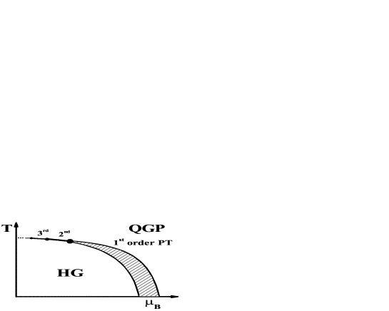
Figure 6: The hypothetical phase diagram of strongly interacting matter in the $T-\mu_{B}$ plane with strangeness taken into account. The line of the 1^st order phase transition is transformed into a ”strip”. For further details see caption of Fig. 5.

The lower and upper limits of the ”strip” are defined, respectively, by the conditions:

$$s_{H}(T,\mu_{B},\mu_{S}^{H})~{}=~{}s_{Q}(T,\mu_{B},\mu_{S}^{H})~{},~{}~{}~{}~{}s_{Q}(T,\mu_{B},\mu_{S}^{Q})~{}=~{}s_{H}(T,\mu_{B},\mu_{S}^{Q})~{}.$$ (68)

The $T$ and $\mu_{B}$ values inside the ”strip” correspond to the mixed HG-QGP phase for which the following conditions have to be satisfied:

$$s_{H}(T,\mu_{B},\mu_{S})~{}=~{}s_{Q}(T,\mu_{B},\mu_{S})~{},$$ (69)

$$n_{S}^{mix}~{}\equiv~{}\delta\cdot~{}n_{S}^{Q}~{}+~{}(1~{}-~{}\delta)\cdot~{}n_{S}^{H}~{}=~{}\delta\cdot~{}T~{}\frac{\partial s_{Q}}{\partial\mu_{S}}~{}+~{}(1-\delta)\cdot~{}T~{}\frac{\partial s_{H}}{\partial\mu_{S}}~{}=~{}0~{},$$ (70)

where $\delta$ is a fraction of the mixed phase volume occupied by the QGP. Eq. (69) reflect the Gibbs equilibrium between the two phases: the thermal equilibrium (equal temperatures), the mechanical equilibrium (equal pressures), the chemical equilibrium (equal chemical potentials). The net strangeness does not vanish in each phase separately, but the total net strangeness of the mixed phase (70) is equal to zero. This means the strangeness–anti-strangeness separation inside the mixed phase GKS . The line (66) for the 2^nd and higher order PTs (i.e. for $1<\alpha\leq 2$) remains unchanged as $\mu_{S}^{H}$ becomes equal to $\mu_{S}^{Q}$ along this line.

VI Summary and Outlook

The phase diagram of strongly interacting matter was studied within the exactly solvable statistical model of the quark-gluon bags. The model predicts two phases of matter: the hadron gas at a low temperature $T$ and baryonic chemical potential $\mu_{B}$, and the quark-gluon gas at a high $T$ and/or $\mu_{B}$. The order of the phase transition is expected to alter with a change of the $\mu_{B}/T$ ratio. The line of the 1^st order transition at a high $\mu_{B}/T$ is followed by the line of the 2^nd order phase transition at an intermediate $\mu_{B}/T$, and then by the lines of the ”higher order transitions” at a low $\mu_{B}/T$. The condition of the strangeness conservation transforms the 1^st order transition line into the ”strip” in which the strange chemical potential varies between the QGP and HG values.

In the high and low temperature domains the approach presented here reduces to two well known and successful models: the hadron gas model and the bag model of QGP. Thus, one may hope the obtained results concerning properties of the phase transition region may reflect the basic features of nature.

Clearly, a further development of the model is possible and required. It is necessary to perform quantitative calculations using known hadron states. These calculations should allow to establish a relation between the model parameters and the $T$ and $\mu_{B}$ values and hence locate the critical line in the $T-\mu_{B}$ plane. Further on one should investigate various possibilities to study experimentally a rich structure of the transition line predicted by the model.

Acknowledgments
We are grateful to V.V. Begun, C. Greiner, E.V. Shuryak, M. Stephanov, and I. Zakout for useful comments and Marysia Gazdzicka for corrections. The work was supported by US Civilian Research and Development Foundation (CRDF) Cooperative Grants Program, Project Agreement UKP1-2613-KV-04 and by the Virtual Institute VI-146 of Helmholtz Gemeinschaft, Germany.

References

- (1) J. C. Collins and M. J. Perry, Phys. Rev. Lett. 34, 1353 (1975).
- (2) for a recent review see: Proceedings of the 17th International Conference on Ultra-Relativistic Nucleus-Nucleus Collisions, Quark Matter 2004, Oakland, California, USA, 11–17 January 2004, editors H. G. Ritter and X.-N. Wang, J. Phys. G30, S633 (2004).
-
(3)
S. V. Afanasiev et al. [The NA49 Collaboration],
Phys. Rev. C 66, 054902 (2002)
[arXiv:nucl-ex/0205002],
M. Gazdzicki et al. [NA49 Collaboration], J. Phys. G 30, S701 (2004) [arXiv:nucl-ex/0403023]. -
(4)
M. Gazdzicki and M. I. Gorenstein,
Acta Phys. Polon. B 30, 2705 (1999)
[arXiv:hep-ph/9803462],
M. I. Gorenstein, M. Gazdzicki and K. A. Bugaev, Phys. Lett. B 567, 175 (2003) [arXiv:hep-ph/0303041]. -
(5)
J. Bartke et al., CERN-SPSC-2004-038, SPSC-EOI-001 (2003),
J. Dainton et al., CERN-SPSC-2005-010. - (6) M. Stephanov, Acta Phys. Polon. B 35, 2939 (2004).
-
(7)
Z. Fodor and S. D. Katz,
JHEP 0203, 014 (2002)
[arXiv:hep-lat/0106002],
F. Karsch, C. R. Allton, S. Ejiri, S. J. Hands, O. Kaczmarek, E. Laermann and C. Schmidt, Nucl. Phys. Proc. Suppl. 129, 614 (2004) [arXiv:hep-lat/0309116]. - (8) A. Chodos et al, Phys. Rev. D 9 (1974) 3471.
- (9) E.V. Shuryak, Phys. Rep. 61 (1980) 71; J. Cleymmans, R. V. Gavai, and E. Suhonen, Phys. Rep. 130 (1986) 217.
- (10) J. Cleymans and H. Satz, Z. Phys. C 57 (1993) 135; J. Sollfrank, M. Gaździcki, U. Heinz, and J. Rafelski, ibid. 61 (1994) 659; G.D. Yen, M.I. Gorenstein, W. Greiner, and S.N. Yang, Phys. Rev. C 56 (1997) 2210; F. Becattini, M. Gaździcki, and J. Solfrank, Eur. Phys. J. C 5 (1998) 143; G.D. Yen and M.I. Gorenstein, Phys. Rev. C 59 (1999) 2788; P. Braun-Munzinger, I. Heppe and J. Stachel, Phys. Lett. B 465 (1999) 15; P. Braun-Munzinger, D. Magestro, K. Redlich, and J. Stachel, ibid. 518 (2001) 41; F. Becattini, M. Gaździcki, A. Keränen, J. Mannienen, and R. Stock, Phys. Rev. C 69 (2004) 024905.
- (11) R. Hagedorn, Nuovo Cimento Suppl. 3 (1965) 147.
- (12) S. Frautschi, Phys. Rev. D 3 (1971) 2821.
- (13) M.I. Gorenstein, V.K. Petrov, G.M. Zinovjev, Phys. Lett. B 106 (1981) 327.
- (14) R. Hagedorn and J. Rafelski, Phys. Lett. B 97 (1980) 136.
- (15) J.I. Kapusta, Phys. Rev. D 23 (1981) 2444.
- (16) D.H. Rischke, M.I. Gorenstein, H. Stöcker, and W. Greiner, Z. Phys. C 51 (1991) 485.
- (17) K.A. Bugaev, M.I. Gorenstein, I.N. Mishustin, and W. Greiner Phys. Rev. C 62 (2000) 044320; Phys. Lett. B 498 (2001) 144.
- (18) K.A. Bugaev, nucl-th/0406033; K.A. Bugaev, L. Phair and J.B. Elliott, nucl-th/0406034; K.A. Bugaev and J.B. Elliott, nucl-th/0501080.
- (19) M.I. Gorenstein, G.M. Zinovjev, V.K. Petrov, and V.P. Shelest Teor. Mat. Fiz. (Russ) 52) (1982) 346.
- (20) M.I. Gorenstein and S.I. Lipskih, Yad. Fiz. (Russ) 38 (1983) 1262; M.I. Gorenstein, Yad. Fiz. (Russ) 39 (1984) 712;
- (21) M.I. Gorenstein, W. Greiner and Shin Nan Yang, J. Phys. G 24 (1998) 725.
-
(22)
L.D. Landau, E.M. Lifschitz,
Statistical Physics (Fizmatlit, Moscow, 2001);
W. Greiner, L. Neise, H. Stöcker Thermodynamik und Statistische Mechanik, Verlag Harri Deutsch, Frankfurt, 1. Auflage (1987). - (23) M.I. Gorenstein, S.I. Lipskih and G.M. Zinovjev, Z. Phys. C 22 (1984) 189.
- (24) K.S. Lee and U. Heinz, Phys. Rev. D 47 (1993) 2068.
- (25) C. Greiner, P. Koch, and H. Stöcker, Phys. Rev. Lett. 58 (1987) 1825.