Polarized quark distributions in nuclear matter

Abstract

We compute the polarized quark distribution function of a bound nucleon. The Chiral Quark-Soliton model provides the quark and antiquark substructure of the nucleon embedded in nuclear matter. Nuclear effects cause significant modifications to the polarized distributions including an enhancement of the axial coupling constant.

Polarized lepton-nucleus scattering experiments are an important tool in hadronic physics. For example, in order to study the spin structure function of the neutron, one must use nuclear targets. It is already well known that there are significant differences betweeen free and bound nucleons in the unpolarized case; the famous European Muon Collaboration (EMC) effect Aubert:1983xm is the prime example. It is reasonable to assume that nuclear effects could appear in polarized quark distributions. Our purpose here is to calculate the analogous modification to the nucleon spin structure function $g_{1}^{(p,n)}(x,Q^{2})$: a ‘polarized EMC effect’.

The first discussion of nuclear effects in the polarized quark distributions is in Ref. Close:1987ay in the context of dynamical rescaling. A more recent calculation Cloet:2005rt predicts dramatic effects for the bound nucleon spin structure function. We have shown Smith:2003hu ; Smith:2004dn that sea quarks, introduced at the model scale, can have important consequences for modifications in the nuclear medium. We will use our previous work Smith:2003hu as a basis for the results presented here, and provide a mechanism for the modification within the Chiral Quark-Soliton (CQS) model Kahana:dx ; Birse:1983gm ; Diakonov:2000pa ; Christov:1995vm ; Alkofer:1994ph . This relativistic mean field approximation to baryons has many desirable qualities such as the inclusion of antiquarks (which is deeply linked to satisfying sum rules and the positivity of Generalized Parton Distributions), and a basis in QCD Diakonov:2000pa . We have previously shown how the model describes nuclear saturation properties, reproduces the EMC effect, and satisfies the bounds on unpolarized nuclear antiquark enhancement provided by Drell-Yan experiments Smith:2003hu . Therefore, we expect the CQS model to produce a reasonable result for the polarized distributions.

The CQS model Lagrangian with (anti)quark fields $\overline{\psi},\psi$, and profile function $\Theta(r)$ is

$$\mathcal{L}=\overline{\psi}(i\partial\!\!\!\!\!\>/\,-Me^{i\gamma_{5}\bm{n}\cdot\bm{\tau}\Theta(r)})\psi,$$ (1)

where $\Theta(r\rightarrow\infty)=0$ and $\Theta(0)=-\pi$ to produce a soliton with unit winding number. The quark spectrum consists of a single bound state and a filled negative energy Dirac continuum; the vacuum is the filled negative continuum with $\Theta=0$. In both the free nucleon and vacuum sectors the positive continua are unoccupied. The wave functions in this spectrum provide the input for the quark and antiquark distributions used to calculate the nucleon structure function.

We work to leading order in the number of colors ($N_{C}=3$), with $N_{f}=2$, and in the chiral limit. While the former characterizes the primary source of theoretical error, one could systematically expand in $N_{C}$ to calculate corrections. We also expect that since the nucleon size is stable in the limit $N_{C}\rightarrow\infty$, the quark wavefunctions, our primary focus, should be within a few percent of their $N_{C}=3$ value Diakonov:2005eq . We take the constituent quark mass to be $M=0.42\text{ GeV}$, which reproduces, for example, the $N$-$\Delta$ mass splitting at higher order in the $N_{C}$ expansion, and other observables Christov:1995vm . We ignore contributions from the structure functions of pion quanta, which in this model propagate through constituent quark loops; they are suppressed by factors of $\mathcal{O}(1/N_{C})$, and are not treated at leading order.

The theory contains divergences that must be regulated. We use a single Pauli-Villars subtraction as in Ref. Diakonov:1997vc because we follow that work to calculate the quark distribution functions. The Pauli-Villars mass is determined by reproducing the measured value of the pion decay constant, $f_{\pi}=0.093\text{ GeV}$, with the relevant divergent loop integral regularized using $M_{PV}\simeq 0.58\text{ GeV}$. This regularization also preserves the completeness of the quark states Diakonov:1997vc .

The results for binding and saturation of nuclear matter have been published elsewhere Smith:2003hu ; Smith:2004dn , but we provide a brief review for completeness. The nucleon mass is given by a sum of the energy of a single valence level ($E^{v}$), and the regulated energy of the soliton ($E_{\Theta}$ equal to the energy in the negative Dirac continuum with the energy in the vacuum subtracted)

$$M_{N} = N_{C}E^{v}+E_{\Theta}(M)-\frac{M^{2}}{M_{PV}^{2}}E_{\Theta}(M_{PV})$$ (2)

$$E_{\Theta}(M) = N_{C}\sum_{E<0}E_{n}-E_{n}^{(0)}\Big{|}_{M}.$$ (3)

The field equation for the profile function is

$$\Theta(r)=\arctan\frac{\rho_{ps}^{q}(r)}{\rho_{s}^{q}(r)+g_{s}P_{s}^{N}(k_{F})},$$ (4)

where $\rho_{s}^{q}\text{ and }\rho_{ps}^{q}$ are the quark scalar and pseudoscalar densities, respectively. The dependence of nucleon properties on the nuclear medium has been incorporated in the model by simply letting the quark scalar density in the field equation (4) contain a constant, but Fermi momentum $k_{F}$ dependent, contribution, $P_{s}^{N}(k_{F})$, equal to the convolution of the nuclear scalar density with the nucleon quark density

$$P_{s}^{N}(k_{F})=\int d^{3}r^{\prime}\rho_{s}^{N}(r^{\prime})\rho_{s}^{q}(r-r^{\prime})$$ (5)

arising from other nucleons present in symmetric nuclear matter. This models a scalar interaction via the exchange of multiple pairs of pions between nucleons, and the parameter $g_{s}$ is varied to obtain nuclear saturation.

The nucleon scalar density is determined by solving the nuclear self-consistency equation

$$\rho_{s}^{N}=4\int^{k_{F}}\frac{d^{3}k}{(2\pi)^{3}}\frac{M_{N}(\rho_{s}^{N})}{\sqrt{k^{2}+M_{N}(\rho_{s}^{N})^{2}}}.$$ (6)

The dependence of the nucleon mass, and any other properties calculable in the model, on the Fermi momentum $k_{F}$ enters through Eq. (6). Thus there are two coupled self-consistency equations: one for the profile, Eq. (4), and one for the density, Eq. (6). These are iterated until the change in the nucleon mass Eq. (2) is as small as desired for each value of the Fermi momentum. We use the Kahana-Ripka (KR) basis Kahana:be to evaluate the energy eigenvalues and wave functions used as input for the densities, nucleon mass, and quark distributions.

We introduce a phenomenological vector meson (with mass fixed at $m_{v}=0.77\text{ GeV}$ and coupling $g_{v}$) Walecka:qa exchanged between nucleons, but not quarks in the same nucleon (i.e. we ignore the spatial dependence of the vector field in the vicinity of a nucleon, treating only the nuclear mean field). The vector meson couples to the vector density

$$P_{v}^{N}(k_{F})=\int d^{3}r^{\prime}\rho_{v}^{N}(r^{\prime})\rho_{v}^{q}(r-r^{\prime})=\frac{2k_{F}^{3}}{3\pi^{2}}.$$ (7)

This mechanism is a proxy for uncalculated soliton-soliton interactions used to obtain the necessary short distance repulsion which stabilizes the nucleus.

The polarized quark distribution for flavor $i$ is defined by the difference between the quark distributions with spin parallel $(\uparrow)$ and antiparallel $(\downarrow)$ to the nucleon

$$\Delta q_{i}(x,Q^{2})=q_{i}^{\uparrow}(x,Q^{2})-q_{i}^{\downarrow}(x,Q^{2}).$$ (8)

The polarized antiquark distribution is defined analogously using $\bar{q}_{i}^{\uparrow}$, and $\bar{q}_{i}^{\downarrow}$. The isovector polarized distribution $\Delta q^{(T=1)}(x)=\Delta u(x)-\Delta d(x)$ is the leading order term in $N_{C}$, with the isoscalar polarized quark distribution $\Delta q^{(T=0)}(x)=\Delta u(x)+\Delta d(x)$ smaller by a factor $\sim 1/N_{C}$ and set to zero. This follows from the fact that the isoscalar combination is normalized to the spin of the nucleon, which is $\mathcal{O}(N_{C}^{0})$, while the isovector combination is normalized to the axial coupling, which is $\mathcal{O}(N_{C}^{1})$ Diakonov:1996sr . Therefore, at the model scale $M_{PV}^{2}\simeq 0.34\text{ GeV}^{2}$, we see that a large portion of the spin is carried by the orbital motion of the constituent quarks in the valence level and the sea Diakonov:2000pa . We will therefore suppress the isospin superscript in the following. The distributions are calculated using the KR basis at $k_{F}=0$ and $k_{F}=1.38\text{ fm}^{-1}$ (see Refs. Smith:2003hu ; Smith:2004dn ) almost exactly as in Ref. Diakonov:1997vc where the quark distribution is given by the matrix element

$$\Delta q(x)=-\frac{1}{3}(2T_{3})N_{C}M_{N}\sum_{n}\langle\psi_{n}|\tau^{3}\gamma_{5}(1+\gamma^{0}\gamma^{3})\delta(E_{n}+p^{3}-xM_{N})|\psi_{n}\rangle,$$ (9)

with the regulated sum taken over occupied states. The eigenvalues $E_{n}$ are determined from diagonalizing the Hamiltonian, derived from the Lagrangian (1), in the KR basis. These are also the eigenvalues that enter into Eq. (2) for the mass. The momentum sum rule (for the unpolarized distribution) is automatically satisfied as long as Eq. (2) defines the mass in the unpolarized analog of Eq. (9), and the same eigenvalues are used in both equations Diakonov:1997vc .

The vector and scalar interactions with the other nucleons in the nucleus at the (low) model scale are implicitly included in the energy eigenvalues in Eq. (9). In the ‘handbag’ diagram for deep inelastic scattering in the parton model language, the quarks in the intermediate state are treated as non-interacting, so how do the nuclear interactions modify the parton distributions? The key point is that all three quarks in the intermediate state undergo evolution in QCD from the same starting scale to the scale of the deep inelastic scattering, and it is this scale that would appear in the Wilson coefficients in the language of the operator product expansion (OPE) picture of deep inelastic scattering. The model for medium modifications presented here represents different boundary conditions on the Wilson coefficients or the parton distributions for free and bound nucleons at the model scale that maintains consistency with the parton model and OPE pictures of deep inelastic scattering. It is worth noting here that these two pictures are already consistent in the free nucleon case since the parton model hypothesis that the quark transverse momenta do not grow with $Q^{2}$ is satisfied Diakonov:1997vc , and our model for medium modifications does not damage this equivalence.

The antiquark distribution is given by $\Delta\bar{q}(x)=\Delta q(-x)$ where the sum is over unoccupied states. The use of a finite basis causes the distributions to be discontinuous. These distributions are smooth functions of $x$ in the limit of infinite momentum cutoff and box size, but numerical calculations are made at finite values and leave some residual roughness. This is overcome in Ref. Diakonov:1997vc by introducing a smoothing function. We deviate from their procedure, and do not smooth the results; instead we find that performing the one-loop perturbative QCD evolution Hagiwara:fs provides sufficient, but not complete, smoothing. Some residual fluctuations due to the finite basis remain visible in our results, and the size of these fluctuations serve as a guide to the size of the error introduced by the method.

These distributions are used as input at the model scale of $Q^{2}=M_{PV}^{2}\simeq 0.34\text{ GeV}^{2}$ for evolution to $Q^{2}=10\text{ GeV}^{2}$. The polarized structure function to leading order in $N_{C}$ is given by

$$g_{1}^{(p,n)} = \frac{1}{2}\sum_{i}e_{i}^{2}\big{(}\Delta q_{i}+\Delta\bar{q}_{i}\big{)}$$ (10)

$$= \pm\frac{5}{18}\Delta q^{NS}+\mathcal{O}(N_{C}^{0})$$ (11)

$$\Delta q^{NS} = \frac{3}{5}\big{(}\Delta u-\Delta d+\Delta\bar{u}-\Delta\bar{d}\big{)}+\mathcal{O}(N_{C}^{0}).$$ (12)

The ratio function is defined to be

$$R_{1}(x,Q^{2}) = \frac{g_{1}^{(p|A)}(x,Q^{2},k_{F})}{Ag_{1}^{(p)}(x,Q^{2},k_{F}=0)},$$ (13)

$$g_{1}^{(p|A)}(x,Q^{2},k_{F}) = \int_{x}^{A}\frac{dy}{y}f(y)g_{1}^{(p)}(x/y,Q^{2},k_{F}).$$

The nucleon momentum distribution $f(y)$ in light polarized nuclei has been calculated in Ref. Saito:2001gv . Here, the nucleon momentum distribution is assumed to be the same as the unpolarized case, as the effects of the spin-orbit force will tend to average out in nuclear matter. We can also justify this approximation in nuclear matter because the zero pressure condition $P^{+}=P^{-}$ for a nucleus with momentum $P$ in the rest frame, which implies the light-cone version of the Hugenholtz-van Hove theorem Miller:2001tg , is still true. Therefore, one expects a distribution $f(y)$ that is peaked at $y\simeq 1$, like those in Ref. Saito:2001gv . This peak location is the dominant effect on the ratio Eq. (13); the remaining details of the function $f(y)$ have only a small effect. Following a light-cone approach valid for any mean field theory of nuclear matter for which the density and binding energy per nucleon are the only input parameters Miller:2001tg one obtains

$$f(y)=\frac{3}{4\Delta_{F}^{3}}\theta(1+\Delta_{F}-y)\theta(y-1+\Delta_{F})\left[\Delta_{F}^{2}-(1-y)^{2}\right],$$ (14)

where $\Delta_{F}=k_{F}/\overline{M}_{N}$ and $\overline{M}_{N}=M_{N}(0)-15.75\text{ MeV}$.

We show the ratio Eq. (13) in Fig. 1 using a ‘valence’-like distribution, as well as for the full distribution. The latter includes all medium modifications, while the former distribution uses the medium modified energy level eigenstate, but the same free nucleon sea quark distribution for both the free and bound nucleon. This was done in order to compare our results with the model in Ref. Cloet:2005rt , which only has valence quarks at the model scale. The single energy level actually has a contribution to the polarized antiquark distribution, so it alone cannot be considered a true valence spin structure function. However, this contribution is small, so we effectively reproduce the result of a valence quark model, especially in the region $x\gtrsim 0.3$.

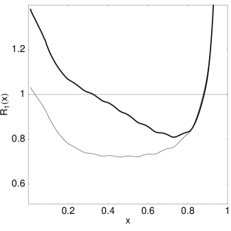
Figure 1: The ratio Eq. (13) at scale $Q^{2}=10\text{ GeV}^{2}$ for nuclear matter. The heavy line is the full calculation for nuclear matter. The light line is the effect calulated using only medium modifications to the ‘valence’ energy level as decribed in the text.

In Fig. 1, one can see that there is a large depletion for $0.3\lesssim x\lesssim 0.7$ in the polarized ‘valence’ quark distribution. This produces a large depletion in the isovector axial coupling $g_{A}^{(3)}$ of $17.8$%. This large effect is comparable to that of the calculation in Ref. Cloet:2005rt which only includes valence quarks at the model scale. This valence effect is mitigated by a large enhancement in the sea quark contribution, so that the full polarized distribution has only a moderate depletion in the region $0.3\lesssim x\lesssim 0.7$ of the same size as the EMC effect in unpolarized nuclear structure functions. There is a large enhancement for $x\lesssim 0.3$ due to the sea quarks. This large enhancement is very different from the small effect calculated in the unpolarized case Smith:2003hu , and seen in unpolarized Drell-Yan experiments Alde:im . This would suggest that one might see a significant enhancement in a polarized Drell-Yan experiment, even after including shadowing corrections (which we address later). The larger sensitivity to the lower components of the wave functions is the primary source for the greater sea quark enhancement in the polarized case, in contrast to the unpolarized case.

The axial coupling $g_{A}^{(3)}$ is enhanced by 9.8% in the nuclear medium. This is in accord with an earlier finding of a $\sim 25$% enhancement for $g_{A}$ in a different soliton model by Birse Birse:1993nr . There, the effect is also seen as a competition between enhancement and depletion. In order to address the medium modification of the Bjorken sum rule Bjorken:1966jh ; Bjorken:1969mm

$$\lim_{Q^{2}\rightarrow\infty}\int_{0}^{1}dx\>g_{1}^{(p)}(x,Q^{2})-g_{1}^{(n)}(x,Q^{2})=\frac{g_{A}}{6}$$ (15)

as an integral of the experimentally observed nuclear distribution, one must account for the effects of shadowing. This occurs when the virtual photon striking the nucleus fluctuates into a quark-antiquark pair over a distance $\sim 1/2M_{N}x$ exceeding the inter-nucleon separation. This causes a depletion in the structure function for $x\lesssim 0.1$ and is relatively well understood Piller:1999wx ; Arneodo:1992wf ; Sargsian:2002wc . Shadowing in the polarized case is expected to be larger than in the unpolarized case by roughly a factor of 2 simply from the combinatorics of multiple scattering (see e.g. Ref. Guzey:1999rq ).

The enhancement at $x\sim 0.1-0.2$ in Fig. 1 is comparable to that seen by Guzey and Strikman Guzey:1999rq ; they assume that the combined effects of shadowing, enhancement, and target polarization lead to the empirical value of the nuclear Bjorken sum rule for ³He and ⁷Li. Shadowing effects become large for $x\lesssim 0.05$, but we ignore them as well as target polarization; such precision is not necessary for our relatively qualitative analysis. One needs $\sim 10$ times the shadowing observed in the unpolarized case for Lead in order to counter the enhancement at $x\sim 0.1-0.2$, and give the same value for the Bjorken sum rule (15) in matter and free space. This assumes that shadowing is the only significant effect neglected at small $x$ in our calculation of the unpolarized quark distribution Smith:2003hu .

We also present, in Fig. 2, the results for the spin asymmetry

$$A_{1}^{(p)}(x,Q^{2})=\frac{\sum_{i}e_{i}^{2}[\Delta q_{i}(x,Q^{2})+\Delta\bar{q}_{i}(x,Q^{2})]}{\sum_{i}e_{i}^{2}[q_{i}(x,Q^{2})+\bar{q}_{i}(x,Q^{2})]}.$$ (16)

The nuclear asymmetry $A_{1}^{(p|A)}$ is defined by replacing the polarized and unpolarized quark distributions, represented generically as $q$, with

$$q^{(p|A)}(x,Q^{2},k_{F})=\int_{x}^{A}\frac{dy}{y}f(y)q^{(p)}(x/y,Q^{2},k_{F}).$$ (17)

We find that for the free case, the calculation falls slightly below the data due to the smaller value of $g_{A}$ in the large $N_{C}$ limit, and that the size of the medium modification is of the same order as the experimental error for the free proton Anthony:2000fn ; Airapetian:1998wi .

Figure 2: The asymmetry $A_{1}^{(p|A)}$ Eq. (16) at scale $Q^{2}=10\text{ GeV}^{2}$. The heavy line is for nuclear matter. The dashed line is for the free proton. The data are for the free proton from SLAC Anthony:2000fn (filled) for $Q^{2}\sim 1-40\text{ GeV}^{2}$ and HERMES Airapetian:1998wi (empty) for $Q^{2}\sim 1-20\text{ GeV}^{2}$ The free curve falls slightly below the data due to the lower value of $g_{A}$ calculated in the large $N_{C}$ limit.

The central mechanism to explain the EMC effect is that the nuclear medium provides an attractive scalar interaction that modifies the nucleon wave function. We see this again in the polarized case. This is also the dominant mechanism in the model of Cloet et al Cloet:2005rt , and the soliton model of Birse Birse:1993nr .

The present model provides a intuitive, qualitative treatment that maintains consistency with all of the free nucleon properties calculated by others Diakonov:2000pa ; Christov:1995vm . It provides reasonable description of nuclear saturation properties, reproduces the EMC effect, and satisfies the constraints on the nuclear sea obtained from Drell-Yan experiments with only two parameters for the nuclear physics ($g_{s}$ and $g_{v}$) fixed by the binding energy and density of nuclear matter. Therefore, we expect the results presented here to manifest themselves in future experiments with polarized nuclei. Our conclusions differ from those in Ref. Cloet:2005rt ; the main difference is the role of sea quarks at the model scale. Therefore, we also expect future experiments would help determine the role of sea quarks in nuclei.

- (1) J. J. Aubert et al., Phys. Lett. B 123, 275 (1983).
- (2) F. E. Close, R. G. Roberts and G. G. Ross, Nucl. Phys. B 296, 582 (1988).
- (3) I. C. Cloet, W. Bentz and A. W. Thomas, arXiv:nucl-th/0504019.
- (4) J. R. Smith and G. A. Miller, Phys. Rev. Lett. 91, 212301 (2003)
- (5) J. R. Smith and G. A. Miller, Phys. Rev. C 70, 065205 (2004)
- (6) S. Kahana, G. Ripka and V. Soni, Nucl. Phys. A 415, 351 (1984).
- (7) M. C. Birse and M. K. Banerjee, Phys. Lett. B 136, 284 (1984).
- (8) D. Diakonov and V. Y. Petrov, in “At the Frontier of Particle Physics, Vol. 1” M. Shifman (ed.), World Scientific, Singapore, pp. 359-415 (2001).
- (9) C. V. Christov et al., Prog. Part. Nucl. Phys. 37, 91 (1996).
- (10) R. Alkofer, H. Reinhardt and H. Weigel, Phys. Rept. 265, 139 (1996)
- (11) D. Diakonov, Eur. Phys. J. A 24S1, 3 (2005).
- (12) D. Diakonov et al., Phys. Rev. D 56, 4069 (1997).
- (13) S. Kahana and G. Ripka, Nucl. Phys. A 429, 462 (1984).
- (14) J. D. Walecka, Annals Phys. 83, 491 (1974).
- (15) D. Diakonov, V. Petrov, P. Pobylitsa, M. V. Polyakov and C. Weiss, Nucl. Phys. B 480, 341 (1996)
- (16) K. Hagiwara et al., Phys. Rev. D 66, 010001 (2002).
- (17) K. Saito, M. Ueda, K. Tsushima and A. W. Thomas, Nucl. Phys. A 705, 119 (2002)
- (18) G. A. Miller and J. R. Smith, Phys. Rev. C 65, 015211 (2002).
- (19) D. M. Alde et al., Phys. Rev. Lett. 64, 2479 (1990).
- (20) M. C. Birse, Phys. Lett. B 316, 472 (1993).
- (21) J. D. Bjorken, Phys. Rev. 148, 1467 (1966).
- (22) J. D. Bjorken, Phys. Rev. D 1, 1376 (1970).
- (23) G. Piller and W. Weise, Phys. Rept. 330, 1 (2000).
- (24) M. Arneodo, Phys. Rept. 240, 301 (1994).
- (25) M. M. Sargsian et al., J. Phys. G 29, R1 (2003).
- (26) V. Guzey and M. Strikman, Phys. Rev. C 61, 014002 (2000)
- (27) P. L. Anthony et al., Phys. Lett. B 493, 19 (2000)
- (28) A. Airapetian et al., Phys. Lett. B 442, 484 (1998)