Resonance and virtual bound state solutions of the radial Schrödinger equation

Abstract

The formulation of the eigenvalue problem for the Schrödinger equation is studied, for the numerical solution a new approach is applied. With the usual exponentially rising free-state asymptotical behavior, and also with a first order correction to it, the lower half of the $k$ plane is systematically explored. Note that no other method, including the complex rotation one, is suitable for calculating virtual bound states far from the origin. Various phenomena are studied about how the bound and the virtual bound states are organized into a system. Even for short range potentials, the free state asymptotical condition proves to be inadequate at some distance from the real $k$ axis; the first order correction doesn’t solve this problem.

Therefore, the structure of the space spanned by the mathematically possible solutions is studied and the notion of minimal solutions is introduced. Such solutions provide the natural boundary condition for bound states, their analytical continuation to the lower half plane does the same for resonances and virtual bound states. The eigenvalues coincide with the poles of the S-matrix. The possibility of continuation based on numerical data is also demonstrated. The proposed scheme is suitable for the definition of the in- and outgoing solutions for positive energies; therefore, also for the calculation of the so called distorted S-matrix in case of long range interactions.

I Introduction

Description of resonances in scattering processes is an inherent part of quantum mechanics N66 , many publications are studying them. The natural way to define a resonance or virtual bound state is provided by the poles of the scattering amplitude in the complex energy variable. Usually, for numerical reasons it is possible to calculate resonances only with a small imaginary part of the energy i.e. the so called ”narrow” resonances. To overcome this limitation the complex rotation method is usedSim73 ; Mois98 . With a non-uniter transformation the energy spectrum is deformed in such a way that any given resonance becomes part of the point spectrum and with proper numerical method its energy can be determined. But the applicability of the method is limited, it is not possible to calculate virtual bound states. In this respect c.f. the explicit statement made in ref.Ser01 : ”Because complex rotation methods cannot give the virtual states, we use a numerical integration of the Schrödinger equation”.

In the present paper the formulation of the eigenvalue problem directly for the Schrödinger equation is studied. For resonances and virtual bound states not only the numerical method to solve the equation is unstable, but also the applied boundary condition at infinity proves to be problematic.

Bound states are defined by two requirements: the wavefunction is regular at the origin and exponentially decreases at infinity. These independent conditions are satisfied only at specific energies. The standard method for finding the eigenvalues can be called ”midpoint matching”. The Schroedinger equation is integrated in two steps: in the internal region from the origin up to a suitably chosen matching point $R_{m}$ and in the external region from a large radius $R_{M}$ inward to $R_{m}$. Since the unwanted other solutions decrease in the chosen directions, the numerical results are accurate and one can easily find those energies where the two solutions concurrent with each other. Naturally, the existence of the $R_{M}\rightarrow\infty$ limit has to be examined.

Unfortunately, for resonances and for virtual bound states the method does not work in this form. The integration in the internal region remains the same, but since these eigenvalues are defined by an exponentially increasing asymptotical behavior, the inward integration in the external region is inaccurate: any small admixture of the asymptoticly decreasing solution catastrophically increases. The loss of accuracy is not critical only if the imaginary part of the wave-number $k$ is small, in other cases one has to restrict the calculation to very limited values of $R_{M}$.

A new effective approach to overcome the above limitation is proposed in the present paper. In its first form this method was proposed in ref.BV95 , but here it is developed further. As an example, it is applied with a short range potential, the Saxon-Woods one, but general problems are addressed. Though the single channel case is considered to be completely understood, the reliable results provided by the numerical method make it necessary to solve some principal problems. Namely, it is necessary to clarify the proper asymptotical behavior of the wavefunctions. The usually supposed ”exponentially rising free-state solution” is only an approximation, valid only for short range potentials near the real $k$ axis.

The cornerstone of the constructions presented is the notion of minimal solutions, a similar notion is used in the theory of three-term recurrence relations JT80 . Since it provides a concise formal way to describe the exponentially decreasing solutions, it is introduced on a relatively early stage. In the two-dimensional linear space spanned by the mathematically possible solutions at a fixed energy, the minimal solutions are those solutions which decrease faster at infinity than the other ones. The minimal solutions form a one-dimensional subspace at energies outside of the positive axis (on the half-axis they obviously do not exist), they provide the natural asymptotical condition for the possible bound states and because of their behavior they can be easily computed.

One can overcome the difficulties present for the inward integration for resonances and virtual bound states by changing the representation of the wavefunction. If sufficiently accurate information on the asymptotical behavior is available, then one can calculate only the correction to this behavior. ”Sufficiently accurate” means that the remainder term is smaller than a minimal solution. Such a representation results in an inhomogeneous differential equation, the behavior of the source term assures that the inward integration is accurate BV95 . Since the asymptotical behavior is used as a reference function for the solution, I propose to call the approach ”reference method”. In the present paper it is pointed out that the formulated method provides accurate results for a wide class of solutions rather than only for that single solution for which the supposed asymptotical behavior is valid.

As usual, accurate numerical results reveal inaccuracies in theoretical understanding: it is necessary to clarify the proper boundary condition for resonances and virtual bound states. At first the usual free-state asymptotical behavior was assumed. Using it an infinite row of resonances with a nearly constant imaginary part is detected. Their position depends on the range parameter of the potential and on the distance where the free-state behavior is imposed, therefore such resonances are clearly unphysical. Since the free-state boundary condition strictly corresponds to the truncation of the potential, one can call them truncation eigenvalues. To ”improve” the boundary condition, a first order correction generated by the exponential asymptotics of the potential is calculated. But the unphysical resonances survived with being pushed downwards. Since the numerical method itself is accurate, the usually neglected subtle problem of the correct boundary condition has to be solved in a general way.

But before that, with the above boundary conditions various phenomena are studied. These include the dependence of the eigenvalue positions on the potential parameters (including collisions), eigenvalues corresponding to the deep potential well behind the centrifugal barrier and depending practically only on the radius of the potential, the node number rules for the virtual bound states, the interrelation between the bound and virtual bound states and so on. The behavior of the eigenvalues in the range singularity generated by the exponential tail of the potential is also studied. Despite the ”approximative” nature of the used boundary conditions, important factual results are received.

It is by no means straightforward to determine the asymptotical behavior for resonances and virtual bound states in a general way. By using only the solution space at fixed energy, it is not possible to find in a natural way somehow an ”other” solution which is different from the minimal one. Time reversal does not help and the only available mathematical structure, namely the symplectic form provided by the Wronski determinant for the solutions, is not sufficient to define an orthogonal subspace to the subspace spanned by the minimal solutions. Analyzing the above presented methods to choose the boundary condition, one can realize that their essence is the continuation of some approximation, which is valid on the upper half-plane, to the lower one. Note that the evaluation of a formula automatically performs an analytical continuation. Therefore the proper condition is provided by the continuation of the ”exact”, i.e. the minimal, solutions to the lower half of the complex wave-number plane. If the wavefunction at $R_{m}$ is continued, one can spare even the inward integration.

In this context the analytical dependence of the solutions was discussed and the feasibility of the continuation to the lower half-plane was successfully demonstrated using data provided by the reference method. Since the solutions are defined by both the value of the wavefunction and its derivative, while the normalization is irrelevant, the continuation is performed for a function with values in what is called ”projective complex plane”.

The principle of continuation for the minimal solutions has an important and unexpected consequence. Minimal solutions can be calculated for any potential, including long range ones, without detailed information on the asymptotics and their continuation to the real $k$ axis provides the ingoing and outgoing solutions. It is straightforward to describe the ”physical solution”, i.e. the solution regular at the origin, as a linear combination of these solutions. The coefficients determine what can be called the ”distorted S-matrix”. In this way one can perform scattering calculations practically for any long range potential, the only prerequisite condition is the existence of minimal solutions outside the positive energy axis.

Finally, it is pointed out that, because of the connection between the minimal and the in- and outgoing solutions, the eigenvalues defined with the continued minimal solution boundary condition coincide with the poles of the S-matrix.

Due to the complex nature of the studied problem, the present paper contains quite a heterogeneous material: from numerics to complex projective planes. Mostly only simple logical steps are used, but to understand them the reader has to be acquainted with the corresponding field. Numerical illustrations are often given, but in fact they play a more important role, they serve as source of information on the studied problem. In this respect numerics plays exactly the same role as measurements do in an experimental study. As far as it was possible, abstract mathematical notions are not used in the interpretation, since it is usual in nuclear physics. But general notions are to express the very essence of the phenomena, therefore they are unavoidable for a deeper understanding.

The present paper is not about the history of the subject. It was not traced back where the results appeared first, some of them could have been received for exactly solvable cases. On the whole, the approach is quite different from the usual one, it is irrelevant if the priority for some particular details belongs to others. The proposed numerical approach (i.e. the reference method used in the first part of the paper), many of the factual results concerning virtual bound states, the formulation of the eigenvalue problem with the boundary condition provided by the analytical continuation of the minimal solutions and the implementation of this continuation for a function with values in $\mathrm{P}\mathbb{C}$ are definitely new.

II Preliminaries, some conventions used in the paper

The Schrödinger equation the solutions of which are sought is

$$\varphi^{\prime\prime}(r)+\biggl{(}k^{2}-V(r)-\frac{L(L+1)}{r^{2}}\biggr{)}\varphi(r)=0$$ (1)

with standard notation. For $V(r)$ the Saxon-Woods potential is chosen as a typical example

$$V(r)=\frac{V_{o}}{1+\exp((r-R_{o})/a)}$$ (2)

Such a form is used to describe the thickness of the nuclear surface layer around $r=R_{o}$. But, as a side effect, the potential has an exponential tail $W_{o}=V_{o}\exp(-\mu r)$, where $\mu=1/a$ and $W_{o}=V_{o}\exp(R_{o}/a)$. Therefore the same $a$ parameter determines the asymptotical behavior too. The phenomena studied in this paper are mostly connected to the asymptotics.

If not stated otherwise, the following values are used for the parameters: $R_{o}=7.5\,\mathrm{fm}$, $\mu=1.4\,\mathrm{fm}^{-1}$. The value for $V_{o}$ is usually $-2.0\,\mathrm{fm}^{-2}$, such a potential is roughly realistic for a nucleon in the ${}^{208}\mathrm{Pb}$ nucleus.

As it is described in the introduction, for the calculation of the eigenvalues a matching procedure is performed, for it the mostly used parameter values are $R_{m}=R_{o}$ and $R_{M}=30.0\,\mathrm{fm}$.

The differential equation uniquely defines the solution if at some, i.e. necessarily finite, point the value of the solution and of its derivative are given. But for the studied problem the boundary condition is imposed at infinity. It is said that a given expression describes the asymptotical behavior of the solution if with this boundary condition imposed at $R_{M}$ the $R_{M}\rightarrow\infty$ limit exists for the solution. With other words, it is implicitly supposed that the remainder term is smaller than any other solution. The basic principal problem addressed in this paper is the the correct asymptotics. For bound states there is no problem since the other solution decreases inwards, but for resonances and virtual bound states it is preferable to formalize the description.

III Structure of the solution space, minimal solutions

At a given energy the solutions of the Schrödinger equation are uniquely defined by the value of the wavefunction and its derivative at a fixed point, the mathematically possible solutions span a two-dimensional vector space. Provided they exists, the so called minimal solutionsJT80 define a one-dimensional subspace in a natural way. An $m(r)$ solution is called minimal, if another $d(r)$ dominant solution exists for which $m(r)/d(r)\rightarrow 0$ at $r\rightarrow\infty$. Any constant multiple of $m(r)$ is minimal, any solution outside of the linear subspace defined by $m(r)$ is a dominant pair to it. Moreover, if there are two solutions which are minimal, then they are necessarily constant multiple of each other. The proof is straightforward: independent $m_{1}(r)$ and $m_{2}(r)$ serve as a basis to expand the corresponding $d_{1}(r)$ and $d_{2}(r)$ functions, but this assumption gives contradicting conditions on $m_{1}(r)/m_{2}(r)$.

It is well known that except for positive real energies minimal solutions do exist. In this paper they are labeled by the wave-number $k$ defined by the energy parameter, $E=k^{2}$. By definition, that sign of the square root is chosen for which $\mathrm{Im}(k)>0$.

Minimal solutions are of great theoretical and practical importance. The usual condition imposed on the asymptotical behavior of a bound state wavefunction assures that it is a minimal solution. Note also, that the regularity condition in the origin also can be interpreted in terms of minimal solutions (of an other type, of course). But what makes minimal solutions really important is the unique property that their value at a given point can be easily calculated by integrating inward from a large distance with a nearly arbitrary boundary condition: despite the presence of a contaminating other solution only the minimal solution survives. While from a theoretical point of view a minimal solution is uniquely defined, for the numerical practice it can be thought of as a bundle of different solutions which all agree to a certain accuracy in a given interval, but which can widely differ at very large distances. In other words, for numerics the minimal solution is a family of different exact solutions.

Resonances and virtual bound states have an asymptotical behavior obviously different from the minimal solution. But it is not straightforward to determine their behavior. Note that to speak of the ”exponentially rising solution” is highly inaccurate, with any admixture of the minimal solution the same property holds. It is always necessary to use some, perhaps implicit, assumption to eliminate this ambiguity. Unfortunately it is not possible to find in a natural way somehow an ”other” solution, different from the minimal one, using only the solution space at fixed energy. The principal reason is that the only mathematical structure, namely the symplectic form provided by the Wronski determinant for the solutions, is clearly not sufficient to define an orthogonal subspace to the subspace spanned by the minimal solutions. In fact, it is possible only in the opposite direction: after one chooses a subspace, is it possible to define a scaler product, like for Kaehler manifolds Simpl . Therefore at first the intuitively obvious, i.e. ”the exponentially rising” free-state solution is chosen and the symptoms provided by it are carefully analyzed. It is not a waste of efforts, during it interesting results are obtained. Only after some information is gathered is it possible to point out that the analytical continuation of the minimal solutions in the energy variable is the principal answer.

IV The reference method

In this section an approach to solve the radial equation in the external region is introduced. The general considerations presented here are applied and therefore illustrated in the next sections.

The basic idea of the method is quite simple: the solution of the Schröedinger equation is formally split into two terms $\varphi(r)=f(r)+u(r)$, where $f(r)$ is a fixed reference function and $u(r)$ is the correction function to be calculated. It yields in a trivial way

$$u^{\prime\prime}(r)+\bigl{(}k^{2}-V(r)-\frac{L(L+1)}{r^{2}}\bigr{)}u(r)=s(r),$$ (3)

with $s(r)\equiv-f^{\prime\prime}(r)-\bigl{(}k^{2}-V(r)-\frac{L(L+1)}{r^{2}}\bigr{)}u(r)$. By choosing $f(r)$ and the boundary condition for $u(R_{M})$ in various ways one can influence the behavior, and thus the possible numerical accuracy of the $u(r)$ solution.

At the beginning it is supposed that for the $\varphi(r)$ solution the $\varphi_{a}(r)$ asymptotical behavior is known with an accuracy better than any minimal solution. It means that the $\bigl{(}\varphi(r)-\varphi_{a}(r)\bigr{)}/m(r)\rightarrow 0$ relation holds at $r\rightarrow\infty$ for some minimal solution $m(r)$. Obviously, this condition is in agreement with the definition of the asymptotical behavior made in section II. In this case the above scheme with $f(r)=\varphi_{a}(r)$ and with the $u(R_{M})=0,u^{\prime}(R_{M})=0$ (i.e with the $\varphi(R_{M})=\varphi_{a}(R_{M}),\varphi^{\prime}(R_{M})=\varphi^{\prime}_{a}(R_{M})$) boundary condition can be applied. Since $u(r)=\varphi(r)-\varphi_{a}(r)$, during an inward integration the correction function rises faster than the minimal solutions.

To discuss the propagation of numerical errors, recall that the general solution of an inhomogeneous equation is a particular solution (e.g. the solution with the $u(R_{M})=0,u^{\prime}(R_{M})=0$ boundary condition) plus the general solution of the homogeneous equation. One can think of a single numerical integration step as a stochastic source of small solutions of the homogeneous equation, while the further steps are accurate to the contaminated solution. ”Small” means that both the function and its derivative are small. The introduced contamination can be represented as linear combination of the complete solution $\varphi(r)$ and of $m(r)$. It means that any possible error can propagate inwards at most as a minimal solution. The presence of the $\varphi(r)$ admixture is not dangerous, it slightly influences only the norm of the result. But in the generic case even a small admixture of $m(r)$ can be catastrophic.

In the given case $u(r)$ is rising faster than the minimal solutions, therefore the relative contribution of the contaminating solution is fading out in case it is sufficiently small and it is considered sufficiently far from the place of its admixture. Moreover, a similar statement is valid for the relative error introduced by a slightly inaccurate boundary condition for $u(r)$. Therefore, in any point far from $R_{M}$, let us say at $R_{m}$, the numerical error is defined only by the accuracy of the nearby integration steps. With other words, in case of $R_{M}\rightarrow\infty$ the limit for the solution exist.

The reference method is not a numerical one in the strict sense. Only the differential equation is reformulated in order to influence the behavior of that part of the solution which is numerically calculated. The resulting inhomogeneous equation can be solved with any available numerical method,in the present paper the standard Runge-Kutta-Fehlenberg one was used. When high accuracy was needed, a high order routine was chosen.

A great advantage of the proposed integration scheme is that for any given reference function one can easily check in a empirical way if there is a corresponding solution simply by comparing the correction function to a minimal solution. With other words, there is no need to derive the reference function in an exact way, an a posteriori check is possible.

One can also exploit the freedom provided by the boundary condition for $u(R_{M})$. Since the integration of the minimal solution is stable, one can describe its presence by including it into the boundary condition. If its relative weight is sufficiently large, than at $R_{m}$ it is still present in the result (with a small numerical error, of course). To get the $R_{M}\rightarrow\infty$ limit, however, one has to choose its weight correspondingly. It means that it is not necessary to adhere to the solution the asymptotical behavior of which is defined by the used reference function, the space of solutions for which the integration is stable is larger. Note also that the minimal solution component in the boundary condition can be replaced by any of the numerically equivalent solutions mentioned in section III.

One can go even further and incorporate not just the minimal solutions into the boundary condition. In this case the simplest approach is to express the boundary condition in terms of the reference function and a fixed minimal solution, consequently apply a renormalization of the reference function and therefore the source term too. It makes possible to accurately perform the inward integration for an arbitrary boundary condition.

V A naive approach: free-state boundary condition

At first the usual naive approach is adopted: it is supposed that the asymptotical behavior of the virtual bound and resonant states is provided by the ”exponentially rising” solution of the free equation. Namely, for $L=0$ the asymptotical behavior is given by $\varphi_{a}(r)=\exp(ikr)$. In case of a short range potential and near the real $k$ axis it is an adequate condition. For the correction function the reference method yields the inhomogeneous equation

$$u^{\prime\prime}(r)+(k^{2}-V(r))u(r)=\exp(ikr)V(r)$$ (4)

It is assumed that the boundary condition is $u(R_{M})=0,u^{\prime}(R_{M})=0$ at some large but necessarily finite $R_{M}$.

Figure 1: Stability of the integration schemes at $k=-i\cdot 0.6\;\mathrm{fm}^{-1}$. Free-state boundary condition results are given by triangles, the corresponding functions are marked by a zero index, the iterated boundary condition results are given by inverse triangles and marked by index one. The open symbols give the correction functions, the full ones the complete wavefunctions. The solid line gives a minimal solution, any error can increase during its propagation at most according to it. Due to the different boundary conditions the complete solutions are different, but the rough logarithmic scale hides it. Apart from the normalization, the deviation between their values is the order of 4%.

Details of the numerical integration for the external region at $k=-i\cdot 0.6\;\mathrm{fm}^{-1}$ are presented in fig.1. It can be seen that the method is numerically stable: any error introduced at some $r$ can propagate inwards rising at most as a minimal solution $m(r)$. But due to the presence of the source term, $u(r)$ rises faster. This proves a posteriori that there is a solution of the Scröedinger equation which has the supposed asymptotics.

By taking into account that the asymptotical behavior of the solutions is $\exp(\pm ikr)$, simple straightforward considerations as well as an empirical check show that the stability region for the above integration scheme is $\mathrm{Im}(k)>-\mu/2$. For $k$ values inside this region the limit for $u(R_{m})$ exists at $R_{M}\rightarrow\infty$, therefore its value can be calculated to an accuracy defined by the nearby integration steps only.

Note that the generalization of the above simple formulation to arbitrary orbital momenta even in the presence of a Coulomb interaction is straightforward: the known solutions for these cases can be chosen as the reference function.

The eigenvalues received by matching the complete external function to the regular wavefunction calculated in the internal region exhibit a suspicious horizontal row just inside the border of the stability region, cf. fig.2. For the Saxon-Woods potential these are not ”physical” resonances, their distance from each other is inversely proportional to $R_{M}$. Since in numerical sense the integration is accurate for such $k$ values, it is only the truncation of the potential, i.e. the free-state boundary condition imposed at finite $R_{M}$, which can be inadequate. This problem shall be studied in detail.

Figure 2: Eigenvalues for L=0. The bound states are given by full circles, the virtual bound states by squares, the empty squares are provided by the free-state boundary condition, while the full squares by the iterated one. The triangles are the non-physical eigenvalues, the inverse triangles are provided by the iterated condition. The sensitivity of the eigenvalue at $k=0.4286-i\cdot 0.6675\;\mathrm{fm}^{-1}$ on $R_{M}$ is demonstrated by the open triangles: they correspond to $R_{M}=25,27.5,32.5\;\mathrm{and}\;35.0\;\mathrm{fm}$.

For nonzero L values interesting phenomena can be studied even with the above simple form of the numerical method. But to make the logical structure of the present paper more transparent, in the next section the elimination of the truncation poles is attempted by improving the supposed asymptotical behavior. A more detailed exploration of the lower half of the $k$ plane is left to the next but one section.

VI Long range effects for a short range potential, iterated boundary condition

It was found in the previous section that the free-state boundary condition imposed at some finite $R_{M}$ value generates unphysical eigenvalues, the position of which strongly depends on $R_{M}$ (cf. fig.2). In this section a correction term is derived for L=0, which describes the singular behavior at $k=-i\mu/2$ and can be used as a reference function for the $\mathrm{Im}(k)>-\mu$ region.

In scattering theory it is usual to rewrite the differential equation for the radial problem in a Volterra-type integral form N66 . The advantage is that it contains the boundary condition too. The equation with the $\exp(ikr)$ boundary condition at infinity is

$$\begin{split}\varphi(r)&=\exp(i\cdot kr)+\frac{i}{2k}\times\\ &\times\biggl{(}\exp(i\cdot kr)\int\limits_{r}^{\infty}\exp(-i\cdot kx)V(x)\varphi(x)\,dx-\exp(-i\cdot kr)\int\limits_{r}^{\infty}\exp(i\cdot kx)V(x)\varphi(x)\,dx\biggr{)}\end{split}$$ (5)

Of course, this equation is meaningful only if $\mathrm{Im}(k)>-\mu/2$. If only the exponential tail of the Saxon-Woods potential is taken into account, the first iteration of eq.(5) is

$$\varphi(r)\rightarrow\varphi(r)_{a}=\exp(i\cdot kr)\biggl{(}1+\frac{W_{o}}{\mu(\mu-i\cdot 2k)}\exp(-\mu r)\biggr{)}$$ (6)

Strictly speaking, this formula is derived with the above limitation on $k$, nevertheless one can heuristically consider it in a larger region.

The iterated asymptotics is singular at $k=-i\mu/2$, which corresponds to the well known singularity of scattering in exponential potentials N66 . Since for the eigenvalue problem the normalization is irrelevant, the pole is considered to be automatically removed by a factor of $\mu(\mu-i\cdot 2k)$. But some kind of singular behavior still remains: it shall be discussed later.

Previously it was established, that the free-state solution can be used as reference function for the numerical integration at $\mathrm{Im}(k)>-\mu/2$. The iterated asymptotics is more accurate, therefore it is meaningful to use it as a new reference function. The calculation of the new source term is straightforward, details can be found in BV95 . A direct comparison of the minimal solution at the same energy and the calculated new correction function with the $u(R_{M})=0,u^{\prime}(R_{M})=0$ boundary condition shows that the latter is rising faster during the inward integration now for $\mathrm{Im}(k)>-\mu$ (cf. fig.1). Consequently, for the wavefunction the $R_{M}\rightarrow\infty$ limit exists in this region. The better description of the asymptotical behavior results in a larger stability region for the new scheme. It should be emphasized that it was proved only that the new reference function correctly describes the asymptotics of some solution in a wider region, but absolutely no information is received whether that is the solution needed for the definition of resonances.

When the singularity on the imaginary $k$ axis at $k=-i\mu/2$ is passed from above, a zero of the wavefunction moves to infinity and below it returns as a minimum (cf. fig.3). For every finite $R_{M}$ there is an interval when not the rising free-state solution describes the behavior there: it is a typical long-range effect. Obviously, it cannot be described if any approximation is introduced which alters the the potential around infinity. Note that not only the structure of the solution is changed, i.e. a node disappears, but in the singularity the boundary condition coincides with that of a bound state with the same energy. Some consequences of this anomalous behavior shall be studied in the next section. It is interesting that despite the presence of a singularity, the calculated wavefunction varies smoothly at $R_{m}$; even the disappearing zero crosses sufficiently earlier.

Figure 3: Behavior of the complete external wavefunction around the range singularity at $k=-i\mu/2$. The numbers at the curves give the value of $k$ on the imaginary axis.

The free-state and the iterated boundary conditions give nearly the same matching condition for $\mathrm{Im}(k)\gtrsim-0.5\>\mathrm{fm}^{-1}$. At $k=-i\,\cdot\,0.6\>\mathrm{fm}^{-1}$ the difference between the two cases is still only 4% (cf. fig.1). But in the immediate neighborhood of $k=-i\,\cdot\,0.7\>\mathrm{fm}^{-1}=-i\mu/2$ the two wavefunctions behave quite differently. Note that it is impossible to prove in a strict mathematical sense which case is ”correct”, since it concerns the definition of the eigenvalue problem. Only a careful analysis of the consequences combined with physical intuition can guide us.

To make the comparison of the two approaches easier, the eigenvalues calculated with the iterated boundary condition are also given in fig.2. The horizontal row of the unphysical resonances now pushed further downwards to the border of the new stability region. The sensitivity to the value of $R_{M}$ remains, of course. It means that one can consider the iterated boundary condition ”better” than the free-state one, but the subtle problem of the proper boundary condition for resonances is not solved by the iteration.

VII Exploration of the lower half of the $k$ plane.

In this section some factual results received with the ”approximative” boundary conditions studied so far are collected. These results are not directly related to the problem of the correct asymptotics, nevertheless they are interesting in themselves and they complement to the general picture. Due to limitations on space, only some aspects can be discussed, even such important phenomenon as the existence of the centrifugal eigenvalues is presented only fragmentary.

VII.1 Node numbers and the system of bound and virtual bound states.

The node number is defined only for real valued functions i.e. only for wavefunctions on the imaginary $k$ axis. It is straightforward to count the zeroes. For bound states the well-known rule is that the ground state has no zero, with increasing energy for every next bound state the node number is increased by one. The $\varphi(\infty)=0$ boundary condition for the regular solution can be interpreted as the appearance of a zero at infinity at that energy, therefore bound states divide the negative energy axis into sectors, where the regular solutions have equal node numbers. Because the node at infinity (and possibly at the origin) is not counted by definition, the bound state lies at the upper edge of the corresponding sector. A virtual bound state is also regular, its node number is defined by the sector corresponding its energy.

When the strength of the potential is increased, bound and virtual bound states usually arise in a collision of a resonance state with its time-reversed pair, i.e. with that state which is located symmetrically to the imaginary $k$ axis. For $L=0$ the collision takes place on the negative imaginary axis, in other cases in the origin. Just after the collision the states have equal node numbers. In case $L=0$ two virtual bound states are formed, one of them moves downward on the imaginary $k$ axis, while the other moves upward and after crossing the origin becomes a bound state. Because of the sector structure, the energy of the corresponding virtual bound state is always lower than that of the bound state. In some sense the virtual bound state is locked in its sector: the regularity in itself defines the solution, normally the energy of a bound state cannot coincide with the energy of a virtual bound state, consequently it is not possible to move into the neighboring sector in a simple way. Note that such a behavior is independent of the the virtual bound state asymptotics, it entirely follows from the regularity condition in the origin. In the following subsections two cases shall be studied when specific circumstances make possible for the virtual bound state to leave its native segment.

VII.2 Exploration of the lower half of the complex $k$ plane for L=4.

The modification of the numerical scheme with the free-state reference function to nonzero $L$ values is straightforward: well-known Hankel functions replace the simple exponential behavior. Despite the restriction to $\mathrm{Im}(k)\geqq-\mu/2$ wave-number values, some interesting phenomena can be studied.

Figure 4: Eigenvalues for L=4 with free-state asymptotics. ”Ordinary” (i.e bound, virtual bound and resonant in the usual sense) eigenvalues are given by full circles, the ground state at $i\cdot 0.904\;\mathrm{fm}^{-1}$ is not presented. The ”unphysical” eigenvalues are given by triangles, the ”centrifugal” ones by squares. At the empty square an eigenvalue is expected from similar results for the pure square well potential, but it was not found here.

The eigenvalues calculated for a relatively large orbital momentum, $L=4$, are presented in fig.4. By changing different parameters of the potential one can study their nature and divide them into different groups. Besides the bound and virtual bound states, the horizontal row of equidistant eigenvalues generated by the free-solution boundary condition appears here too. In addition, the position of some other eigenvalues depends predominantly on the $R_{o}$ radius parameter and is practically insensitive to the $V_{o}$ strength of the potential. Obviously, these eigenvalues are generated by the deep potential well behind the centrifugal barrier, therefore one can call them centrifugal eigenvalues. And there are eigenvalues, (for instance, in fig.4 the one at $k=0.74-i\,\cdot\,0.37\;\mathrm{fm}^{-1}$ ), which along a power-like trajectory approaches the imaginary axis when the strength parameter is increased, collides there with its symmetric pair and one member of the colliding pair becomes the newest bound state, while the other changes into a virtual bound state. With increasing strength this virtual state moves downward the negative imaginary axis, cf. fig.5.

Figure 5: Eigenvalue trajectories and the centrifugal barrier eigenvalue on the imaginary axis, L=4. The virtual bound state pair of the first exited state is given by triangles, the centrifugal eigenvalue by circles. The solid line corresponds to the exited state and gives the boarder of the sectors with one and with two node-numbers. While the colliding eigenvalues are off the imaginary axis, the imaginary part of their position is given by diamonds, an error bar defines the real parts of their positions.

But for nonzero even $L$ values one of the centrifugal eigenvalues is located on the imaginary axis itself and disturbs the movement of the virtual bound state. In fact, they collide, leave the imaginary axis, describe a small loop in the complex plane, after returning to the imaginary axis they collide again. One of them remains near the previous place while the other continues its way downward the axis: the complicated choreography is needed for changing the node number of the wavefunctions. When the virtual bound state approaches the centrifugal barrier eigenvalue, the two states have equal node numbers. After the collision they leave the imaginary axis, but somewhat later they return. Off the axis the wavefunction is complex, there are no nodes. While they are off the axis, the bound state on the positive imaginary axis crosses this energy region, therefore when they return, they are located in a different sector, i.e. their node number is increased by one. Now the centrifugal barrier eigenvalue is ”ready to face” the next virtual bound state with an increased node number. Note that the virtual bound state continues its way down the imaginary $k$ axis, but now on the other side of the corresponding bound state, i.e. with a increased node number. This example illustrates how the eigenvalues are organized into a system.

VII.3 Eigenvalue structures for different boundary conditions, L=0.

This case provides a possibility to illustrate that the boundary condition for the wavefunction can be chosen independently of the reference function, as it has been already discussed in section IV.

With the free-state solution as the reference function one can stably integrate the equation only for the $\mathrm{Im}(k)\geqq-\mu/2$ region. To achieve stability for the larger $\mathrm{Im}(k)\geqq-\mu$ region one has to use the iterated asymptotics. To find the eigenvalues with the free-state boundary condition in the larger domain, it is possible to choose the boundary condition for the correction function appropriately . I chose the $u(R_{M})=0,u^{\prime}(R_{M})=W_{o}\mu\exp((ik-\mu)R_{M})$ condition, the results for the larger region are also presented in fig 2. The virtual bound states are locked into their own native segments and there is a tendency to approximate the lower bound state. In fig.2 all of the three free-state boundary condition defined virtual bound states given by empty squares are extremely near to these bound states.

In case of the iterated asymptotical behavior, the boundary condition for the virtual bound state in the singularity at $k=-i\mu/2$ is practically the same as for the bound state, therefore in this case the two states can coincide. Moreover, they should coincide: a bound state eigenvalue there implies a virtual bound state too, and vice versa. It is illustrated in fig.6 that a bound state reaches the energy of the singularity simultaneously with a virtual bound state, the virtual state sheds a zero, leaves its native segment and enters the segment defined by the bound state. This is an other example of how a virtual bound state can change its node number.

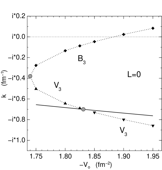
Figure 6: Eigenvalue trajectories and the iterated singularity, L=0. The state which becomes the third exited state is given by diamonds, its virtual bound state pair by triangles. The solid line gives the segment boarder defined by the second exited state. Large half filled circle denotes the area where entering of $\mathrm{V}_{3}$ into the segment of $\mathrm{B}_{2}$ takes place; during the crossing even the wavefunctions coincide. A similar circle denotes the formation of $\mathrm{B}_{3}$ and $\mathrm{V}_{3}$ in a collision of two resonances.

Therefore the virtual bound states can be extremely sensitive to the asymptotical behavior of the potential. In fig.2 the states which correspond to the fourth bound state $\mathrm{B}_{3}$ and which are located at $k=-i\cdot 0.79\,\mathrm{fm}^{-1}$ and at $k=-i\cdot 0.91\,\mathrm{fm}^{-1}$ seem to be not far from each other, nevertheless they are completely different: the node numbers are 3 and 2.

The ground state arises not in a collision of two resonances, but the corresponding eigenvalue is generated directly as a virtual bound state while the potential is still extremely weak. For example, at $V_{o}=-0.0001\,\mathrm{fm}^{-2}$ there is a virtual bound state at $k=-i\cdot 0.51\,\mathrm{fm}^{-1}$. At the same time, there is no other eigenvalue on the imaginary axis in the stability region of the numerical method. To avoid any misunderstanding, it should be emphasized that such a weak potential generates only a small perturbation of the internal and external wavefunctions, typically it alters only the fifth digits. The eigenvalue arises as the concurrence of these slightly perturbed wavefunctions. With increasing strength of the potential this virtual bound state moves towards the origin and eventually becomes the ground state.

In contrast, the presence of the centrifugal barrier for $L\neq 0$ modifies the genesis of the ground state. At very week potential only the more or less fix centrifugal eigenvalues arise, the ground state comes from a pair which collide at $k=0$.

VIII Analytical behavior of the solutions

It is timely to look in perspective at how the asymptotical behavior is chosen for the eigenvalue problem. Because of the stability, for bound states different possibilities are feasible. It is usual to suppose that the exponentially decreasing free-state solution provides the asymptotics. But note that even the $\varphi(R_{M})=0$ boundary condition can be used. The minimal solutions also provide a more sophisticated asymptotics.

On the lower half-plane resonances and virtual bound states are, as a rule, instable, the free-state boundary condition is not satisfactory. An improved approximation of the asymptotical behavior was introduced, it proved to be inadequate too: the unphysical eigenvalues are not eliminated. Therefore the iteration process can not solve the principal problem of the proper boundary condition. It seems obvious that the minimal solutions contain in some form the information still missing from the iterated asymptotics, but unfortunately these are defined only on a different half-plane.

VIII.1 Principle of analytical dependence of the solutions

At different energies the minimal solutions are completely independent: their normalization is arbitrary. Therefore the values at fixed $r$ do not provide an analytical function of the $k$ variable. Even if such a normalization is used which provides analytical values, in the generic case the derivatives are not necessarily analytical. But if both the values and the derivatives happen to be analytical, this behavior is preserved when the solutions are integrated to a different $r$ because the Schrödinger equation contains the $k$ parameter in an analytical form. Unfortunately, I cannot give due reference in the literature to this ”obvious” statement. In some sense minimal solutions can be considered to be the limits of solutions with the $\varphi(R_{M})=0,\varphi^{\prime}(R_{M})=\text{const.}$ boundary condition. Therefore, if the normalization constants are correctly chosen, minimal solutions provide an analytical function of the $k$ parameter. Of course, the choice is not unique, but it concerns only the normalization, a property irrelevant for the eigenvalue problem. Once an analytical dependence is achieved, the solutions can be continued to such regions of the $k$ variable where they were originally not defined. This continuation is essentially (i.e. apart from the normalization) unique.

On the analytical dependence a constraint can be imposed. For real potentials and for real energies the solutions can be chosen to be real. Usually, the minimal solutions at negative energies are considered to be real, I follow this practice. Because they are real, at some fixed $r$ value the wavefunctions satisfy the basic constraint

$$\varphi(k,r)=\varphi^{\ast}(-k^{\ast},r)$$ (7)

where asterisk denotes the complex conjugation. Since not only the left hand, but also the right hand side is an analytical function of the $k$ variable, the equation holds everywhere. In presence of branch points, however, one should carefully follow the possibly different sheets of $k$ and $k^{\ast}$.

The just formulated basic constraint is in fact the consequence of time reversal symmetry. But when Wigner studied time reversal (cf. ref.Wig , for instance) only real physical quantities were considered. Therefore, he derived the $\varphi\rightarrow\varphi^{\ast}$ and the $k\rightarrow-k$ transformation rules. The later differs from the $k\rightarrow-k^{\ast}$ rule suggested by the above formula. The extra complex conjugation is the principal reason that time reversal does not help in defining a solution different from the minimal one, since it maps the minimal subspace onto a minimal subspace at different energy rather than into the solution space at the same energy.

VIII.2 Continuation of the minimal solutions

The free-state solutions describe the asymptotical behavior not only for the minimal solutions, but they provide sufficiently accurate asymptotics on the real $k$ axis too. Therefore they were also used for the boundary condition in the lower half-plane. Note that the evaluation of an explicit formula with an argument in the lower half-plane is equivalent with an analytical continuation. It means that a continuation procedure has been already applied. But somewhere the continuation of an approximation can considerably deviate from the continuation of the function itself. A better approximation, the iterated asymptotics, gave satisfactory results in a larger domain. It needs, however, calculations using information on the potential itself and resulting in explicit formulas to be able to perform the continuation.

A convenient way to deal with this difficulty can be just the opposite approach: a continuation based on ”raw” numerical values of the minimal solutions accurately calculated, let us say, at $R_{m}$ rather than at $R_{M}$. It saves even the inward integration and provides directly the matching condition.

In approximation theory of analytical functions W60 the phenomenon of ”superconvergence” is well known. If a function is considered on a domain, the rate of convergence for any possible polynomial approximation sequence is limited by the nearest singularity. A sequence reaching the possible fastest rate is called converging ”maximally”. The base theorem is that any maximally converging polynomial sequence converges to the continued function in a larger domain, of course, with a smaller rate of convergence. By the geometry of the domain and by the nearest singularity this rate is defined in a relatively complicated manner (cf. chapter IV in ref.W60 ). Note that the superconvergence theorem provides no effective error estimate, the accuracy should be checked by other means.

Exploiting the phenomenon of superconvergence an ”empirical” continuation was applied to measured nuclear reaction data (cross sections and polarizations) to extract structure information in a model independent way B76 ; BG89 . The interested reader is referred to the cited literature, B76 is perhaps the first choice. But to understand the present paper all that subtlety of convergence rate estimates and optimal conformal mappings together with the various methods to check the reliability of the results are not needed.

To illustrate the possibilities, numerical results provided by the iterated boundary condition are used with $R_{M}=35\,\mathrm{fm}$ and $V=2.0\,\mathrm{fm}^{-2}$. The solutions at $R_{m}=7.5\,\mathrm{fm}$ are defined by two ordered complex numbers, $\varphi(k,R_{m})$ and $\varphi^{\prime}(k,R_{m})$, one of them is nonzero and the normalization is irrelevant. One’s first guess is to fit $\varphi/\varphi^{\prime}$ with a rational fraction $\mathrm{P}_{n}(k)/\mathrm{Q}_{m}(k)$, where $\mathrm{P}_{n}(k)$ and $\mathrm{Q}_{m}(k)$ are polynomials of order $n$ and $m$. The difficulty with this approach is that the result is not symmetric, i.e. a fit to $\varphi^{\prime}/\varphi$ with $\mathrm{Q}_{m}(k)/\mathrm{P}_{n}(k)$ gives a different result. The reason is that in the complex plane the distance of $\varphi/\varphi^{\prime}$ and $\mathrm{P}_{n}(k)/\mathrm{Q}_{m}(k)$ is different from the distance of $\varphi^{\prime}/\varphi$ and $\mathrm{Q}_{m}(k)/\mathrm{P}_{n}(k)$. A solution to this problem is presented in the appendix. Maximal convergence can be achieved using somewhat different approximation criteria, therefore other possibilities are also feasible.

Figure 7: Extrapolation of the minimal solutions to the lower half-plane. The calculated values for the complete wavefunction $\phi$ and its derivative $\phi^{\prime}$ at $R_{m}$ on the imaginary $k$ axis are given by circles and triangles, respectively. The solid lines are fitted fifth degree polynomials; the full symbols give fitted values, they were fitted together with other ones in the complex $k$ plane; the empty symbols give values calculated for checking the quality of the extrapolation. For details see the main text.

In the $k$ plane an equidistant grid was used at $k=0.1\cdot(n+i\cdot k)$ with $n,k=0,1,2,\dotsc$. The fitted points were chosen on the border and inside a triangle defined by three points $0.0+i\cdot 0.1$, $0.0+i\cdot 0.6$ and $0.6+i\cdot 0.1$, altogether 28 ones. The used large $R_{M}$ value assured that in these points the minimal solutions themselves were calculated. The fitting polynomials are of the fifth degree, it needs 11 fitted real parameters (because the functions are real for imaginary $k$). The relative accuracy of the fit is typically $10^{-5}$ inside the triangle, $5\cdot 10^{-5}$ in its peaks. The performance of the continuation to the lower half-plane was checked on the imaginary axis by comparing to calculated values (cf. fig.7). Even in the farthest point the accuracy is $10^{-3}$! It might be surprising, nevertheless nothing unexpected happened.

First of all, the base region for the extrapolation (i.e. the region where the fit was performed) contains 28 accurately calculated points, its dimensions just equal the distance of extrapolation. It means that large amount of information was used and the distance of extrapolation is moderate. Secondly, the circumstances are favorable. Apparently, there is no singularity nearby, in the singularity at $k=-i\mu/2$ the function which was extrapolated is regular and the next possible singularity is at $k=-i\mu$. On the whole, one can expect such a good performance, nevertheless the small number of parameters needed is quite promising.

The performed check provides information on the iterated boundary condition too. The facts that practically the minimal solutions themselves are continued and the good agreement with the calculated values in the lower half-plane indicate that in this region one can apply the iterated boundary condition. With other words, a mutual check is performed.

I do not want to make the impression that continuation is a simple procedure. The idea that one should analytically continue some function into an other region for solving different problems in physics is not new. A quite early example can be found in ref.Ch58 , for instance. There has been numerous attempts since then, most of them failed in some sense or another. There are some pitfalls, irresponsible applications not taking them into account and not checking the results carefully can do much harm (c.f. some applications reviewed in refs.B76 ; BG89 ). Due to limitations on space, no introduction to this complicated subject can be given here. Basically, there are four possibilities for checking the performance. First of all, the shape and position of the base region for the continuation can be altered, the independent variable can be changed using a suitably chosen conformal mapping, the contribution of the nearby singularities can be suppressed with multiplicative factors, and finally one can examine the performance of the continuation in such directions where direct calculation is still possible. In this respect the fact that the function to be continued can be accurately calculated practically in a whole half-plane provides unique possibilities. But there is no need to apply any of them here, since a direct check was performed.

IX Implications for scattering calculations: a novel approach

For short range potentials the so called ”outgoing” solutions are the continuation of the minimal solutions to the positive part of the real $k$ axis, while the ”ingoing” solutions are the continuation to the negative part. For long range potentials the continued functions can be considered as the definition of the ingoing and outgoing solutions, for pure Coulomb potential the known solutions satisfy this condition. It means that the calculation of scattering processes was implicitly also treated above. For it the regular wavefunction of the internal region at $R_{m}$ should be described as a linear combination of the outgoing and ingoing solutions rather then only one of them, as in the case of the eigenvalue problem. The coefficients of the linear combination determine the S-matrix, to be exact, the so called ”distorted” S-matrix. The basic constraint imposed on the minimal solutions assures that the normalization ambiguity has no effect, the Wronskian for the in- and outgoing solutions can also be used to fix the normalization. In this way the S-matrix can be easily computed even for quite ”exotic” interactions, the only prerequisite condition is the existence of minimal solutions.

The connection between the minimal and the in- and outgoing solutions shows that an eigenvalue defined with the continued minimal solution boundary condition coincides with a pole of the S-matrix. The S-matrix is a ratio of two coefficients, a pole arises when a zero of the denominator occurs. It is just the definition of the eigenvalue: in the asymptotical behavior only one of the linearly independent minimal and continued minimal solutions is present.

For short range potentials with their free-state asymptotics it is straightforward to calculate ”observable quantities” from the S-matrix. But long range potentials influence the kinematics of the scattering, to be able to calculate observables one has to know the ”physical interpretation”. Such an interpretation is performed when the complete wavefunction is separated into the ”incoming” and the ”scattered” components, while the physical quantities are calculated from them. A clear illustration of it is provided by the standard treatment of the Coulomb case. As a result, observables are defined not only by the ”Coulomb distorted S-matrix”, but also by ”Coulomb phases”.

Hopefully, these considerations help to take into account Coulomb interactions quite accurately also in three-particle calculations. The leading terms (and only the leading terms) of the asymptotics for various components are well studied, a somewhat detailed discussion can be found in ref.VKR01 . The characteristic exponentially rising and decreasing behavior is present, therefore minimal-type solutions should exist. But now the solution space is not two-dimensional, i.e. its structure is more complicated, a stable inward integration of a minimal-type solution is not so simple and straightforward. Therefore, much has to be done to implement the new scheme in a three-particle calculation, only the main steps are clear.

X Conclusions

In the present paper resonances and virtual bound states are studied by considering the eigenvalue problem for the Schrödinger equation. It requires the correct boundary condition for the formulation and an accurate numerical method to solve the equation.

A new and effective approach, the reference method, is developed to solve the equation. Even in its simplest form, i.e. with the free-state reference function, it is suitable to explore the lower half of the complex $k$ plane, in the neighborhood of the imaginary axis too. Keeping in mind the extreme simplicity of the numerical approach, one wonders what is the reason that it was proposed only quite lately and why it is not the standard method for solving the eigenvalue problem, let us say, from the mid-sixties of the last century. Note that even the complex rotation method, usually considered to be very powerful, is not suitable to calculate virtual bound states.

The reliable results provided by the method reveal that not the free-state asymptotical behavior defines resonances and virtual bound states, even for short range potentials. The free-state behavior should be considered only approximative, it is more or less accurate only near the real $k$ axis. The existence of eigenvalues depending on $R_{M}$ clearly shows it. The first iteration of the Volterra-type integral form of the Schrödinger equation provides a correction to the free-state boundary condition. Numerical calculations show that the unphysical eigenvalues survive, only their position is modified.

Despite the approximative nature of the boundary conditions discussed so far, the reference method can provide interesting information. The lower half of the $k$ plane was explored, some results are collected in a separate section. Since the bound and virtual bound states satisfy the same boundary condition at the origin, their position is not independent. Therefore the system they form was studied and also how it changes with increasing strength of the potential.

Nearly fixed eigenvalues describing the potential well behind the centrifugal barrier were found. For nonzero even orbital momenta a complicated choreography of collisions, in which a virtual bound state and the centrifugal eigenvalue take part, was observed . In the collision process the node numbers are increasing.

On the contrary, the virtual bound state sheds a node when crosses the range singularity generated by the exponential tail of the potential. Moreover, in the moment of crossing its wavefunction coincides with the wavefunction of a bound state at the same energy. Such an exotic behavior can influence the nuclear surface.

To find the correct boundary condition, it is necessary to study the structure of the solution space. It is straightforward to define in a simple and natural way the minimal solutions. They provide the natural boundary condition for the bound states. But to find an ”other” solution, which can be used for resonances and virtual bound states, is not straightforward. Neither time reversal nor the symplectic structure provided by the Wronski determinant can help. Carefully analyzing the situation one concludes that the correct condition is given by the analytical continuation of the minimal solutions from the upper half-plane to the lower one. In some sense this conclusion is the main result of the present paper: one can formulate the eigenproblem simultaneously for the bound, the resonant and the virtual bound states.

The principle of analytical dependence provides practical means too. Numerical information on the minimal solutions was used and they were continued to the lower half of the $k$ plane, where the results were compared to the solutions calculated with the reference method using the iterated boundary condition. In this way it was demonstrated that one can effectively perform the continuation. Obviously, the successful continuation of the minimal solutions, i.e. the matching condition itself, means that one can successfully calculate resonances and virtual bound states too.

The importance of the continuation procedure lies not in making obsolete the integration with the aid of the reference method. In many cases the free-state reference function (or its generalization in presence of a Coulomb potential) is accurate enough. For the nuclear structure calculation practice its is usually irrelevant whether the exponential tail for a phenomenological potential is correctly taken into account. If phenomena directly connected to the region just outside of the surface layer (i.e to the 10-13 fm region in fig.3) are studied, then one can apply the iterated asymptotics as the reference function. In this way it is quite safe to apply the simple and transparent reference method for the numerical integration, rather then to perform the relatively unknown continuation. But the latter, i.e. the continuation, is very useful if no free-state type solutions are explicitly known. At complex energies one can easily calculate the minimal solutions, their continuation to the lower half-plane provides the necessary matching condition.

The analytical continuation approach provides unique possibilities for scattering calculations. An important new scheme follows from it in a simple way. Since the in- and outgoing solutions are the continuation of the minimal solutions to the real $k$ axis, one can represent the physical solution, which is regular at the origin, as a linear combination of them, even if the analytical form is unknown. The ”distorted” S-matrix is provided by the ratio of the corresponding coefficients. This scheme is not restricted to the radial equation, but to implement it in more complicated cases some technical problems have to be solved.

Finally, it simply follows from the definitions that the eigenvalues defined with the analytically continued minimal solution boundary condition coincide with the poles of the S-matrix.

Appendix A Least squares for the projective complex plane

As it was discussed above, the solutions are defined by two ordered complex numbers, $\varphi(k,R_{m})$ and $\varphi^{\prime}(k,R_{m})$, one of them is nonzero and the normalization is irrelevant. This is a typical example of what is called complex projective plane and denoted by $\mathrm{P}\mathbb{C}$. If the reader is acquainted with modern differential geometry, he can easily realize that by the stereographic projection a diffeomorfizm onto a two dimensional sphere $S^{2}$ is constructed and the metric of the embedding three dimensional space $\mathbb{R}^{3}$ is used. Below only the algorithm is described.

The elements of $\mathrm{P}\mathbb{C}$ are denoted by (v,w), while elements in $\mathbb{R}^{3}$ are given by their coordinates (x,y,z). A two dimensional sphere $S^{2}$ defined by $x^{2}+y^{2}+(z-1/2)^{2}=1/4$ is also considered.

• If $w\neq 0$ calculate $(x_{1}=\mathrm{Re}(v/w),y_{1}=\mathrm{Im}(v/w),z_{1}=0)$ and consider the straight line connecting this point with the (0,0,1) point on $S^{2}$. Calculate $(x_{v}=x_{1}t_{1},y_{v}=y_{1}t_{1},z_{v}=1-t_{1})$ with $t_{1}=(x_{1}^{2}+y_{1}^{2}+1)^{-1}$. This point is the intersection with the surface of $S^{2}$ and gives the result of the mapping.

• If $v\neq 0$ calculate $(x_{2}=\mathrm{Re}(w/v),y_{2}=-\mathrm{Im}(w/v),z_{2}=1)$ and consider the straight line connecting this point with the (0,0,0) point on $S^{2}$. Calculate $(x_{w}=x_{2}t_{2},y_{w}=y_{2}t_{2},z_{w}=t_{2})$ with $t_{2}=(x_{2}^{2}+y_{2}^{2}+1)^{-1}$. This point is the intersection with the surface of $S^{2}$ and gives the result of the mapping.

• If neither $v$ nor $w$ equals zero, than because of the different sign in formulas for $y_{1}$ and for $y_{2}$ the two mappings define the same image point, i.e. it is irrelevant which one is chosen. Numerical accuracy prefers to divide by that component the absolute value of which is larger.

The last step is to calculate the distance between a fixed and a fitting point in $\mathrm{P}\mathbb{C}$ as the $\mathbb{R}^{3}$ distance of their images on $S^{2}$. It is a smoother function then the distance on the surface of $S^{2}$. As usual, the function to be minimized is the sum of the squared distances.

- (1) R. G. Newton, Scattering theory of waves and particles (McGraw-Hill, New York, 1966).
- (2) B. Simon, Ann. Math. 97, 247 (1973).
- (3) N. Moiseyev, Phys. Rep. 302, 211 (1998).
- (4) P. Serra, S. Kais, and N. Moiseyev, Phys. Rev. A 64, 062502 (2001).
- (5) I. Borbély and T. Vertse, Comp. Phys. Com. 86, 61 (1995).
- (6) W. B. Jones and W. J. Thron, Continued Fractions, Analytic Theory and Applications (Addison-Wesley, London, 1980).
- (7) V. Guillemin and Sh. Sternberg, Symplectic Techniques in Physics (Cambridge University Press, Cambridge, 1984).
- (8) E. P. Wigner, Group Theory and its Application to the Quantum Theory of Atomic Spectra (Academic Press, New York, 1959).
- (9) J. L. Walsh, Interpolation and Approximation by Rational Functions in the Complex Domain, Amer. Math. Soc., New-York 1960.
- (10) I. Borbély, J. of Phys. G5, 937 (1976).
- (11) I. Borbély, W. Grüebler, B. Vuraidel, and V. König, Nucl. Phys. A503, 349 (1989).
- (12) G. F. Chew Phys.Rev. 112, 1380 (1958).
- (13) M. Viviani, A. Kievsky, and S. Rosati, Few-Body Syst. 30, 39 (2001).