Comparison of Nucleon Form Factors from Lattice QCD Against the Light Front Cloudy Bag Model and Extrapolation to the Physical Mass Regime  

Abstract

We explore the possibility of extrapolating state of the art lattice QCD calculations of nucleon form factors to the physical regime. We find that the lattice results can be reproduced using the Light Front Cloudy Bag Model by letting its parameters be analytic functions of the quark mass. We then use the model to extend the lattice calculations to large values of $Q^{2}$ of interest to current and planned experiments. These functions are also used to define extrapolations to the physical value of the pion mass, thereby allowing us to study how the predicted zero in $G_{E}(Q^{2})/G_{M}(Q^{2})$ varies as a function of quark mass.

year number number identifier LABEL:FirstPage1 LABEL:LastPage#131

I Introduction

The electromagnetic form factors of the nucleon are an invaluable source of information on its structure Thomas:2001kw . For example, observing their fall as $Q^{2}$ increases from zero revealed the finite extent of the nucleon, and measuring the Sachs electric form factor of the neutron, $G_{E}^{n}$ Reichelt:2003iw ; Glazier:2004ny , that it has a positive core surrounded by a long-range, negative tail Friedrich:2003iz ; Thomas:1982kv ; cbm . In the last few years particular interest has focused on the ratio of the electric and magnetic form factors of the proton, $G_{E}/G_{M}$, where recoil polarization data Jones:1999rz ; Gayou:2001qd have revealed a dramatic decrease with $Q^{2}$ – in contrast with earlier work based on the Rosenbluth separation. These data have allowed one of us to deduce a fascinating spin dependence of the shape of the nucleon Miller:2003sa .

While the behavior of $G_{E}/G_{M}$ with $Q^{2}$ was anticipated in some models (e.g. see Ref. Frank:1995pv , Chung:1991st ), there is no consensus as to which explanation best represents how QCD works. Direct guidance from QCD itself would be most valuable and for that purpose lattice QCD represents the one and only technique by which one can obtain non-perturbative solutions to QCD.

The QCDSF Collaboration recently presented lattice QCD simulations for the form factors of the nucleon over a wide range of values of momentum transfer QCDSF Collaboration . While these were based on the quenched approximation, with an unsophisticated action, several lattice spacings were chosen with the smallest being around $0.05\operatorname{fm}$ ($\beta=6.4$) and at present these are the state of the art. The quark masses used in the simulations correspond to pion masses in the range $(0.6,1.2)\operatorname{GeV}$. Therefore one needs to parametrize the form factors as a function of pion mass and extrapolate to the physical value before comparing these lattice results with the experimental data.

At $Q^{2}=0$ there have been a number of studies of the chiral extrapolation of baryon magnetic moments  Leinweber:1998ej ; Hackett-Jones:2000qk ; Hemmert:2002uh ; Young:2004tb . However, there is no model independent way to respect the constraints of chiral symmetry over the range of $Q^{2}$ and $m_{\pi}$ required by the QCDSF data. Instead, at finite $Q^{2}$, one has been led to study various phenomenological parameterizations Ashley:2003sn , which have at least ensured the correct leading order non-analytic structure as $m_{\pi}\rightarrow 0$. Our purpose here is three-fold. First, we wish to use the lattice data to investigate whether a particular quark model is capable of describing the properties of the nucleon in this additional dimension of varying $m_{\pi}$ - an important test which any respectable quark model should satisfy. Second, having confirmed that the model is consistent with the lattice data over the range of $m_{\pi}$ noted earlier, we use the model to extrapolate to large values of $Q^{2}$ (for lattice values of $m_{\pi}$). Third, we also use the model to extrapolate to the physical pion mass.

The model which we consider here is the light front cloudy bag model (LFCBM) Miller:2002ig , which was developed as a means of preserving the successes of the original cloudy bag model cbm , while ensuring covariance in order to deal unambiguously with modern high energy experiments. The light front constituent quark model, upon which it is built Frank:1995pv , predicted the rapid decrease of $G_{E}/G_{M}$ with $Q^{2}$ and, as the pion cloud is expected to be relatively unimportant at large $Q^{2}$, this success carries over to the LFCBM Miller:2002ig . Furthermore the LFCBM corresponds to a Lagrangian built upon chiral symmetry, so it can be extended to the limit of low quark mass as well as low and high $Q^{2}$.

The outline of the paper follows. In Sect. 2 we briefly review the LFCBM. In Sect. 3 we present the lattice QCD data, explain the fitting procedure and present the results. Sect. 4 contains some concluding remarks.

II Review of the LFCBM

The light front cloudy bag model (LFCBM) respects chiral symmetry and Lorentz invariance and reproduces the four nucleon electromagnetic form factors. Therefore it is reasonable to try to use it to extrapolate the form factors computed using lattice QCD to the physical pion mass. We begin by briefly introducing the key features of the LFCBM.

The LFCBM is a relativistic constituent quark model incorporating the effect of pion-loops, key features motivated by chiral symmetry. The light-front dynamics is employed to maintain the Poincaré invariance, and one pion-loop corrections are added to incorporate significant pion cloud effects (particularly in the neutron electric form factor and magnetic moments) as well as the leading non-analytic behavior imposed by chiral symmetry. In light-front dynamics the fields are quantized at a fixed “time”$=\tau=x^{0}+x^{3}\equiv x^{+}.$ The light front time or $\tau$-development operator is then $P^{0}-P^{3}\equiv P^{-}$. The canonical spatial variable is $x^{-}=x^{0}-x^{3}$, with a canonical momentum $P^{+}=P^{0}+P^{3}$. The other coordinates are $\mathbf{x}_{\perp}$ and $\mathbf{P}_{\perp}$. The relation between the energy and momentum of a free particle is given by $p^{-}=(p_{\perp}^{2}+m^{2})/p^{+}$, with the quadratic form allowing the separation of center of mass and relative coordinates. The resulting wave functions are frame independent. The light front technique is particularly relevant for calculating form factors because one uses boosts that are independent of interactions.

Our goal is to calculate the Dirac $F_{1}$ and Pauli $F_{2}$ form factors given by:

$$\left\langle N,\lambda^{\prime}p^{\prime}\left|J^{\mu}\right|N,\lambda p\right\rangle=\overline{u}_{\lambda^{\prime}}(p^{\prime})\left[F_{1}(Q^{2})\gamma^{\mu}+\frac{F_{2}(Q^{2})}{2M_{N}}i\sigma^{\mu\nu}(p^{\prime}-p)_{\nu}\right]u_{\lambda}(p)\,.$$ (1)

The momentum transfer is $q^{\mu}=($ $p^{\prime}-p)^{\mu},~{}Q^{2}=-q^{2}$ and $J^{\mu}$ is taken to be the electromagnetic current operator for a free quark. For $Q^{2}=0$ the form factors $F_{1}$ and $F_{2}$ are, respectively, equal to the charge and the anomalous magnetic moment $\kappa$ in units of $e$ and $e/(2M_{N})$ , and the magnetic moment is $\mu=F_{1}(0)+F_{2}(0)=1+\kappa$. The evaluation of the form factors is simplified by using the so-called Drell-Yan reference frame in which $q^{+}=0$, so that $Q^{2}=q_{\bot}^{2}=q_{1}^{2}$. If light-front spinors for the nucleons are used, the form factors can be expressed in terms of matrix elements of the plus component of the current Brodsky:1980zm :

$$F_{1}(Q^{2})=\langle N,\uparrow\left|J^{+}\right|N,\uparrow\rangle,\;\hskip 28.45274pt\mathrm{and}\hskip 28.45274ptQF_{2}(Q^{2})=(-2M_{N})\langle N,\uparrow\left|J^{+}\right|N,\downarrow\rangle\,.$$ (2)

The form factors are calculated using the “good” component of the current, $J^{+}$, to suppress the effects of quark-pair terms. Finally, we note that in our fits we will use the Sachs form factors, which are defined as

$$G_{E}=F_{1}-\frac{Q^{2}}{4M_{N}^{2}}F_{2},\hskip 56.9055ptG_{M}=F_{1}+F_{2}$$ (3)

The next step is to construct the bare (pionless) nucleon wave function $\Psi$, which is a symmetric function of the quark momenta, independent of reference frame, and an eigenstate of the canonical spin operator. The commonly used ansatz is:

$$\Psi(p_{i}) =\Phi(M_{0}^{2})u(p_{1})u(p_{2})u(p_{3})\psi(p_{1},p_{2},p_{3}),$$ (4)

$$p_{i} =\mathbf{p}_{i}s_{i},~{}\tau_{i},$$

where $\psi$ is a spin-isospin color amplitude factor, the $p_{i}$ are expressed in terms of relative coordinates, the $u(p_{i})$ are Dirac spinors and $\Phi$ is a momentum distribution wave function. The specific form of $\psi$ is given in Eq. (12) of Ref. Miller:2002qb and earlier in Ref. Chung:1991st . This is a relativistic version of the familiar SU(6) wave function, with no configuration mixing included. The notation is that $\mathbf{p}_{i}=(p_{i}^{+},$ $\mathbf{p}_{i\bot})$. The total momentum is $\mathbf{P}=\mathbf{p}_{1}+\mathbf{p}_{2}+\mathbf{p}_{3}$, the relative coordinates are $\xi=p_{1}^{+}/(p_{1}^{+}+p_{2}^{+})$, $\eta=(p_{1}^{+}+p_{2}^{+})/P^{+}$, and $\mathbf{k}_{\bot}=(1-\xi)\mathbf{p}_{1\bot}-\xi\mathbf{p}_{2\bot}$, $\mathbf{K}_{\bot}=(1-\eta)(\mathbf{p}_{1\bot}+\mathbf{p}_{2\bot})-\eta\mathbf{p}_{3\bot}$. In computing a form factor, we take quark 3 to be the one struck by the photon. The value of $1-\eta$ is not changed $(q^{+}=0)$, so only one relative momentum, $\mathbf{K}_{\bot}$ is changed: $\mathbf{K}_{\bot}^{\prime}=\mathbf{K}_{\bot}-\eta\mathbf{q}_{\bot}$. The form of the momentum distribution wave function is taken from Schlumpf Schlumpf:1992ce :

$$\Phi(M_{0})={N}{\left(M_{0}^{2}+\beta^{2}\right)^{\gamma}}\,,$$ (5)

with $M_{0}^{2}$ the mass-squared operator for a non-interacting system:

$$M_{0}^{2}=\frac{K_{\bot}^{2}}{\eta(1-\eta)}+\frac{k_{\bot}^{2}+M^{2}}{\eta\xi(1-\xi)}+\frac{M^{2}}{1-\eta}\,.$$ (6)

Schlumpf’s parameters were $\beta=0.607~{}\operatorname{GeV}$, $\gamma=-3.5$, $M=0.267~{}\operatorname{GeV}$, where the value of $\gamma$ was chosen so that $Q^{4}G_{M}(Q^{2})$ is approximately constant for $Q^{2}>4~{}\operatorname{GeV}^{2}$, in accord with experimental data. The parameter $\beta$ helps govern the values of the transverse momenta allowed by the wave function $\Phi$ and is closely related to the rms charge radius. The constituent quark mass, $M$, was primarily determined by the magnetic moment of the proton. We shall use different values when including the pion cloud and fitting lattice data.

A physical nucleon can sometimes undergo a quantum fluctuation so that it consists of a bare nucleon and a virtual pion. In this case, an incident photon can interact electromagnetically with a bare nucleon, Fig. 1a, with a nucleon while a pion is present, Fig. 1b, or with a charged pion in flight, Fig. 1c. These effects are especially pronounced for the neutron $G_{E}$cbm , at small values of $Q^{2}$. The tail of the negatively charged pion distribution extends far out into space, causing the mean square charge radius, $R_{n}^{2}$, to be negative. The effects of the pion cloud need to be computed relativistically if one is to confront data taken at large $Q^{2}$. This involves evaluating the Feynman diagrams of Fig. 1 using photon-bare-nucleon form factors from the relativistic model, and using a relativistic $\pi$-nucleon form factor. The resulting model is defined as the light-front cloudy bag model LFCBM Miller:2002ig . The light-front treatment is implemented by evaluating the integral over the virtual pion four-momentum $k^{\pm},\mathbf{k}_{\perp}$, by first performing the integral over $k^{-}$ analytically, re-expressing the remaining integrals in terms of relative variables ($\alpha=k^{+}/p^{+})$, and shifting the relative _⟂ variable to $\mathbf{L}_{\perp}$ to simplify the numerators. Thus the Feynman graphs, Fig. 1, are represented by a single $\tau$-ordered diagram. The use of $J^{+}$ and the Yan identityChang:qi $S_{F}(p)=\sum_{s}u(p,s)\overline{u}(p,s)/(p^{2}-m^{2}+i\epsilon)+\gamma^{+}/2p^{+}$ allows one to see that the nucleon current operators appearing in Fig.1b act between on-mass-shell spinors.

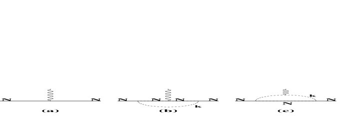
Figure 1: Diagrams

The results can be stated as

$$F_{i\alpha}(Q^{2})=Z\left[F_{i\alpha}^{(0)}(Q^{2})+F_{ib\alpha}(Q^{2})+F_{ic\alpha}(Q^{2})\right],$$ (7)

where $i=1,2$ denotes the Dirac and Pauli form factors, $\alpha=n,p$ determines the identity of the nucleon, and $F_{i\alpha}^{(0)}(Q^{2})$ are the form factors computed in the absence of pionic effects. The wave function renormalization constant, $Z$, is determined from the condition that the charge of the proton be unity: $F_{1p}(Q^{2}=0)=1$. For illustration we start with the calculation of the neutron form factors. Then, evaluating the graph in Fig. 1b gives

$$F_{1bn}(Q^{2})=g_{0}^{2}\int_{0}^{1}d\alpha\alpha\int{\frac{d^{2}L}{(2\pi)^{3}}}R_{N}({\mathbf{L}^{(+)}}^{\;2},\alpha)R_{N}({\mathbf{L}^{(-)}}^{\;2},\alpha)\\ [(F_{1p}^{({0})}(Q^{2})+F_{1n}^{({0})}(Q^{2})/2)(\alpha^{2}(M^{2}-Q^{2}/4)+L^{2})-(F_{2p}^{({0})}(Q^{2})+F_{2n}^{({0})}(Q^{2})/2))(\alpha^{2}Q^{2}/2)],$$ (8)

$$F_{2bn}(Q^{2})=-g_{0}^{2}\int_{0}^{1}d\alpha\alpha\int{\frac{d^{2}L}{(2\pi)^{3}}}R_{N}({\mathbf{L}^{(+)}}^{\;2},\alpha)R_{N}({\mathbf{L}^{(-)}}^{\;2},\alpha)\\ [(F_{1p}^{({0})}(Q^{2})+{\frac{1}{2}}F_{1n}^{({0})}(Q^{2}))(2\alpha^{2}M^{2})\\ +(F_{2p}^{({0})}(Q^{2})+{\frac{1}{2}}F_{2n}^{({0})}(Q^{2})))(\alpha^{2}M^{2}(1-Q^{2}/4M^{2})+(L_{x}^{2}-L_{y}^{2}))]$$ (9)

where $g_{0}$ is the bare $\pi$N coupling constant, and the renormalized coupling constant $Zg_{0}^{2}=g^{2}/4\pi=13.5\;$,$\mathbf{L}_{\perp}^{(\pm)}\equiv\mathbf{L}_{\perp}\pm\alpha\mathbf{q}_{\perp}/2$, $\alpha\equiv{\frac{k^{+}}{p^{+}}}$, $D_{N}(k_{\perp}^{2},\alpha)\equiv{M^{2}\alpha^{2}+k_{\perp}^{2}+\mu^{2}(1-\alpha)}$, and $R_{N}(k_{\perp}^{2},\alpha)\equiv{\frac{F_{\pi N}^{N}(k_{\perp}^{2},\alpha)}{D_{N}(k_{\perp}^{2},\alpha)}}.$ The $\pi$N form factor is taken as Zoller:1991cb ; Szczurek:gw

$$F_{\pi N}(k_{\perp}^{2},\alpha)=e^{{-(D_{N}(k_{\perp}^{2},\alpha)/2\alpha(1-\alpha)\Lambda^{2})}}{,}$$ (10)

and maintains charge conservation Speth:pz . The constant $\Lambda$ is a free parameter, but very large values are excluded by the small flavor asymmetry of the nucleon sea.

From Eqns. (8) and (9) we see that each term in the nucleon current operator contributes to both $F_{1}$ and $F_{2}$. The evaluation of graph 1c yields

$$F_{1cn}(Q^{2})=-g_{0}^{2}F_{\pi}(Q^{2})\int_{0}^{1}d\alpha\alpha\int{\frac{d^{2}K}{(2\pi)^{3}}}R({\mathbf{K}^{(+)}}^{\;2},\alpha)R({\mathbf{K}^{(-)}}^{\;2},\alpha)\left[K^{2}+M^{2}\alpha^{2}-(1-\alpha)^{2}{\frac{Q^{2}}{4}}\right]$$ (11)

$$F_{2cn}(Q^{2})=-g_{0}^{2}(2M^{2})F_{\pi}(Q^{2})\int_{0}^{1}d\alpha\alpha^{2}(1-\alpha)\int{\frac{d^{2}K}{(2\pi)^{3}}}R({\mathbf{K}^{(+)}}^{\;2},\alpha)R({\mathbf{K}^{(-)}}^{\;2},\alpha)$$ (12)

where $\mathbf{K}_{\perp}^{(\pm)}\equiv\mathbf{K}_{\perp}\pm(1-\alpha)\mathbf{q}_{\perp}/2$.

The proton form factors can be obtained by simply making the replacements $n\rightarrow p$ in Eqs. (8,9) and $-g_{0}^{2}\rightarrow g_{0}^{2}$ in Eqs. (11,12). The change in sign accounts for the feature that the $\pi^{-}$ cloud of the neutron becomes a $\pi^{+}$ cloud for the proton. The mean-square isovector radii $\left\langle r^{2}\right\rangle_{i}^{V}$, computed using Eqs. (7), and then taken to the chiral limit at low-$Q^{2}$, have the same singular $\log$ terms as those of the relativistic results of Beg and Zepeda Beg:1973sc .

The LFCBM was defined by choosing four free parameters: $m,\beta,\gamma,\Lambda$ so as to best reproduce the four experimentally measured electromagnetic form factors of the nucleon Miller:2002ig . In the present work, the most relevant of these parameters will be varied to reproduce lattice data, and the resulting dependence on the quark mass and lattice spacing used to extrapolate to the physical region.

III Fitting the QCDSF Form Factors and Extrapolating to the Physical Pion Mass.

In this section we discuss the fitting procedure used to parametrize the nucleon form factors calculated in lattice QCD. We use data produced by the QCDSF Collaboration QCDSF Collaboration and employ the LFCBM to calculate the corresponding form factors, varying the model parameters to find the best-fit to the different sets of lattice data obtained for different values of the current quark mass, $m_{q}$. The behavior of the fitting parameters is then represented by a polynomial function of the quark mass $m_{q}$. This polynomial fit in $m_{q}$, or equivalently in pion mass squared, $m_{\pi}^{2}$, can then be used to extrapolate the values of the fitting parameters to the physical pion mass. Nucleon form factors for the physical pion mass are then calculated using the extrapolated values for the model parameters. In the following few subsections a more elaborate explanation is given and the results are presented. In section III.1 we describe the available data and the analysis procedure used to extract the quantities necessary for further fits. In sec. III.2 we describe the details of the fitting and extrapolation process and in the sec. III.3 we present the nucleon form factors resulting from the extrapolation to the physical pion mass and make comparisons with experiment.

III.1 QCDSF Data and Its Analysis

The form factor calculations in Ref.QCDSF Collaboration  were carried out for three different values of the lattice spacing, $a=\{0.47,0.34,0.26\}\operatorname{GeV}^{-1}$. For each value of $a$ several sets of pion (or equivalently nucleon) masses were considered. For each mass set Dirac and Pauli form factors for both the proton and neutron were calculated at several values of $Q^{2}$. The typical range for the pion mass used varied from $1.2\operatorname{GeV}$ to $0.6\operatorname{GeV}$, with the corresponding nucleon mass ranging from approximately $2\operatorname{GeV}$ to $1.5\operatorname{GeV}$. The typical range for $Q^{2}$ was $0.6\operatorname{GeV}^{2}$ to $2.3\operatorname{GeV}^{2}$.

The LFCBM is basically a relativistic constituent quark model, so we need to relate the model constituent mass of Eq. (6) to the masses of the nucleon and pion. To do so we use the approach of Ref. Cloet:2002eg , ( Eq. (8))

$$M=M_{\chi}+\frac{cm_{q}^{phys}}{(m_{\pi}^{phys})^{2}}m_{\pi}^{2},$$ (13)

where $M_{\chi}$ is the constituent quark mass in the chiral limit, $m_{q}^{phys}$ is the current quark mass and $c$ is of order 1. In the study of octet magnetic moments in the AccessQM model of Ref. Cloet:2002eg , the best fit value for $M_{\chi}$ was $0.42\operatorname{GeV}$, while for $cm_{q}^{phys}$ it was $0.0059\operatorname{GeV}$.

III.2 Lattice Data Fit and Extrapolation

The first step in our extrapolation of the lattice results to the physical quark mass is to fit the lattice results for each quark mass $m_{q}$ by adjusting the parameters of the LFCBM calculation. For that purpose two fitting parameters were chosen. The first parameter is $M_{\chi}$ in Eq. (13), which determines the constituent quark mass. This parameter was varied for each lattice spacing separately, since some dependence upon lattice spacing was anticipated. The second parameter is the internal parameter, $\gamma$, in the nucleon wave function Eq. (5), which is varied separately for each pion (or equivalently nucleon) mass. For convenience, we express all magnetic form factors $G_{M}$ in “physical” units of $e/2M_{N}^{Physical}$. Since the LFCBM uses the mass of the $\rho$-meson included in the pion electromagnetic form factor, we need the extrapolated value for its mass. We use the simple fitting function from Ref. RHO_MASS :

$$m_{\rho}=c_{0}+c_{1}m_{\pi}^{2},$$ (14)

with $c_{0}=0.776\operatorname{GeV}$ and $c_{1}=0.427\operatorname{GeV}^{-1}$ .

A function representing the $\chi^{2}$ for the deviation between the lattice data and the values calculated using the LFCBM was constructed and minimized by varying the fitting parameters. Changing the value of $M_{\chi}$ causes the the calculated form factors to move up or down by an amount approximately independent of $Q^{2}$, thereby causing a relatively small change in $\chi^{2}$. Therefore a simple grid variation for that parameter was employed, with grid boundaries $M_{\chi}\in\left[0.15,0.45\right]\operatorname{GeV}$, and step size of $\delta_{M_{\chi}}=0.01\operatorname{GeV}$. As for the parameter, $\gamma$, the variation of $\chi^{2}$ was much stronger and the Minuit package of CERN’s Root framework ROOT was used for the minimization. At first the boundaries for $\gamma$ were set to keep it in the physical region, but successful boundless runs were also performed in order to confirm the true minimum and error sizes. The pion masses used in the lattice calculation are very large, and the resulting pionic effects are very small. Therefore the value of $\Lambda$ could not be determined from lattice data and its value was held fixed at $\Lambda=0.58\operatorname{GeV}$ Similarly, varying $\beta$ did not change the description of the lattice data, so it was held fixed at $\beta=0.607\operatorname{GeV}/c$. The resulting fits are in good agreement with data, as one can see in Figs. 2, 3, 4 and 5. The best-fit values of the parameters are shown in Table I. The figures show results for the smallest lattice spacing, $a=0.26\operatorname{GeV}^{-1}$, but the reproduction of lattice data is equally successful for larger values of $a$.

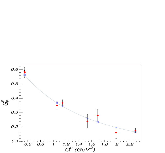
Figure 2: (Color online) LFCBM fit to QCDSF data for $G_{E}^{P}(in~{}units~{}of~{}e)$ for a lattice spacing $a=0.26~{}\operatorname{GeV}^{-1}$, $M_{P}=1.80~{}\operatorname{GeV}$ and $m_{\pi}=0.93~{}\operatorname{GeV}$

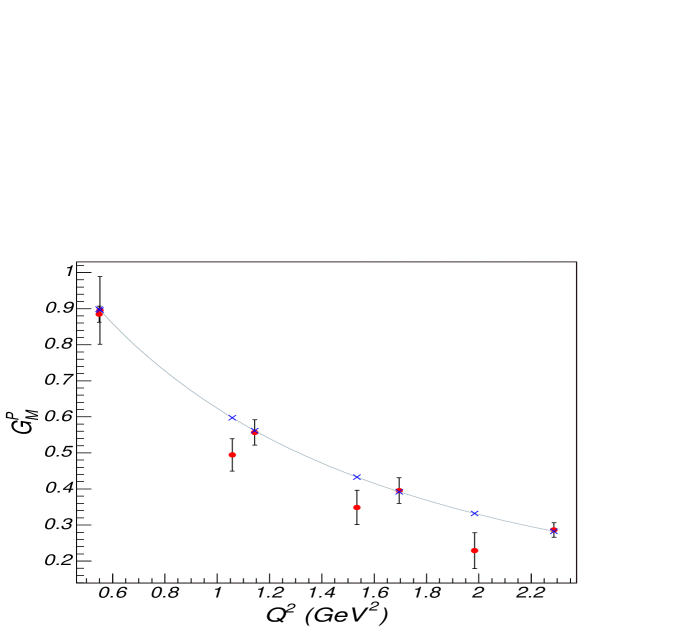
Figure 3: (Color online) LFCBM fit to QCDSF data for $G_{M}^{P}(in~{}units~{}of~{}e/(2M_{N}^{Physical}))$ for a lattice spacing $a=0.26~{}\operatorname{GeV}^{-1}$, $M_{P}=1.80~{}\operatorname{GeV}$ and $m_{\pi}=0.93~{}\operatorname{GeV}$

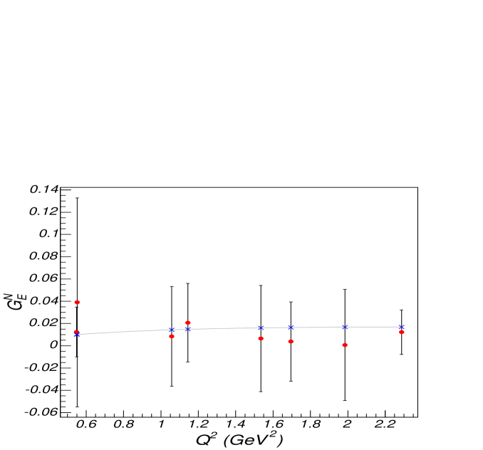
Figure 4: (Color online) LFCBM fit to QCDSF data for $G_{E}^{N}(in~{}units~{}of~{}e)$ for a lattice spacing $a=0.26~{}\operatorname{GeV}^{-1}$, $M_{P}=1.80~{}\operatorname{GeV}$ and $m_{\pi}=0.93~{}\operatorname{GeV}$

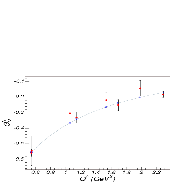
Figure 5: (Color online) LFCBM fit to QCDSF data for $G_{M}^{N}(in~{}units~{}of~{}e/(2M_{N}^{Physical}))$ for a lattice spacing $a=0.26~{}\operatorname{GeV}^{-1}$, $M_{P}=1.80~{}\operatorname{GeV}$ and $m_{\pi}=0.93~{}\operatorname{GeV}$

$$\text{TABLE I.~{}Lattice data and LFCBM fitting parameters.(All expressed in powers of }\operatorname{GeV}\text{.)}$$

$$a$$

The next step is to extrapolate the fitting parameters to the physical quark mass. This is done using the assumption that the parameters vary smoothly as functions of the quark mass, and the fact that $m_{q}\thicksim m_{\pi}^{2}$ over the mass range investigated. We limited the extrapolation function to a low order polynomial in $m_{\pi}^{2}$. The resulting fits for two lattice spacings are presented in Figs. 6 and 7, from which we see that the fitting function provides a very accurate representation of the values obtained from lattice data.

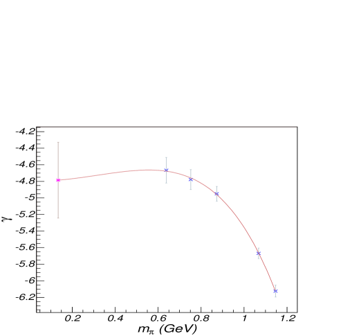
Figure 6: (Color online) Polynomial extrapolation of $\gamma$ vs. $m_{\pi}$ for lattice spacing $a=0.47~{}GeV^{-1}$

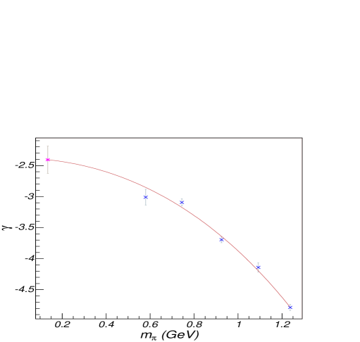
Figure 7: (Color online) Polynomial extrapolation of $\gamma$ vs. $m_{\pi}$ for lattice spacing $a=0.26~{}GeV^{-1}$

The fitted values of $\gamma$ and the extrapolation to the physical value of $m_{\pi}$, with their corresponding errors, are shown in Figs. 6 and 7.

In our calculations, $M_{\chi}$ has a very weak dependence on the pion mass, but it has a rather strong dependence upon the lattice spacing. As we see in Table I and Figs. 2-5, very good fits to the lattice data are obtained even without varying $M_{\chi}$ for each quark mass. By contrast, Fig. 8 and Table I show rather dramatic variation of $M_{\chi}$ for different values of the lattice spacing, $a$. This suggests that the larger values of the lattice spacing are rather far from the continuum limit and (at best) only the results for the smallest lattice spacing should be compared with experimental data. It would clearly be desirable to have new data at even smaller $a$, or using an improved action, known to provide a good approximation to the continuum limit.

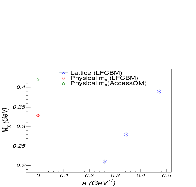
Figure 8: (Color online) Variation of $M_{\chi}$with lattice spacing $a.$The best-fit values of $M_{\chi}$ for physical $m_{\pi}$ using LFCBM and AcessQM models are presented as well.

Use of the values of $\gamma,M$ determined by the lattice data in the LFCBM defines a lattice version of the LFCBM. We may use this new model to compute the form factors at arbitrarily large values of $Q^{2}$, thereby extending the kinematic range of the lattice calculations. The results are shown in Figs. 9, 10, 11 and 12. In Figs. 13 and 14 we show the corresponding plots of $\mu_{0}G_{E}/G_{M}$.

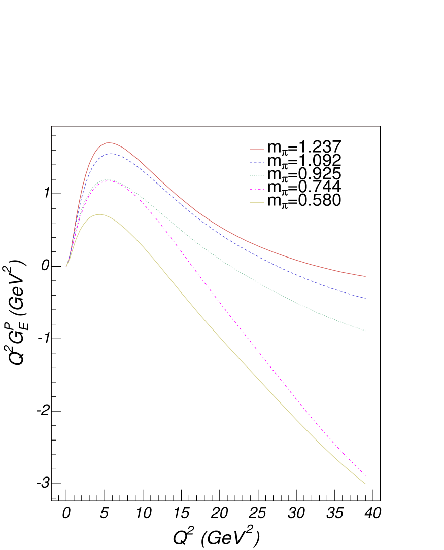
Figure 9: (Color online) LFCBM calculations using parameters (Figs. 6, 7 and 8) obtained by fitting the lattice results for the proton electric form factor, $G_{E}$, at lattice  spacing $a=0.26~{}GeV^{-1}$.

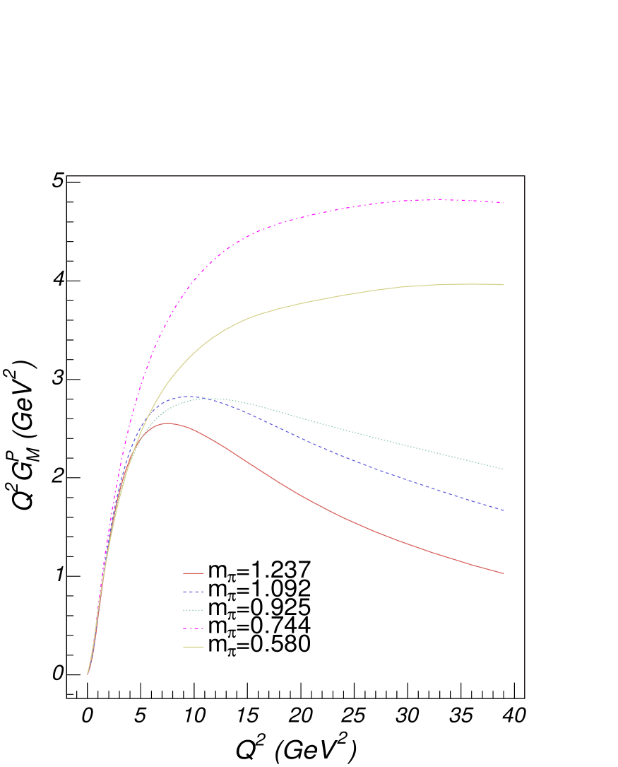
Figure 10: (Color online) LFCBM calculations using parameters (Figs. 6, 7 and 8) obtained by fitting the lattice results for the proton magnetic form factor, $G_{M}$, at lattice  spacing $a=0.26~{}GeV^{-1}$.

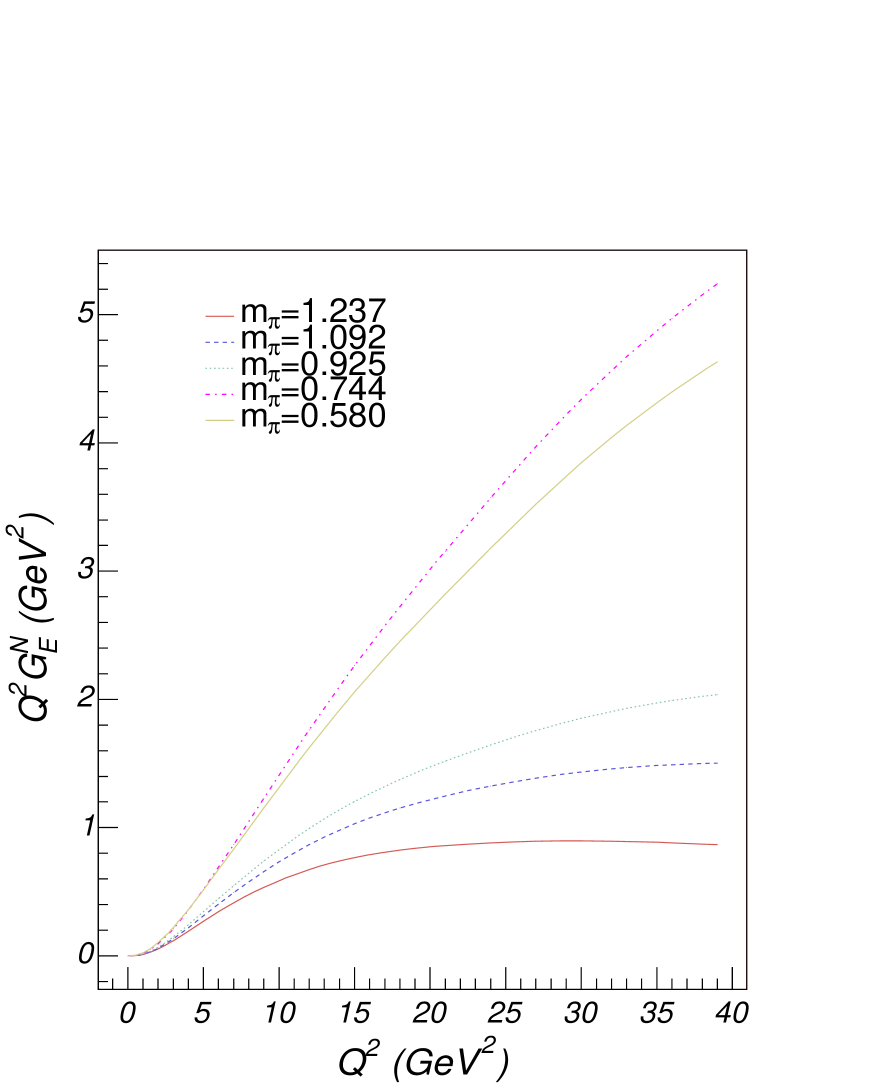
Figure 11: (Color online) LFCBM calculations using parameters (Figs.6, 7 and 8) obtained by fitting the lattice results for the neutron electric form factor, $G_{E}$, at lattice  spacing $a=0.26~{}GeV^{-1}$.

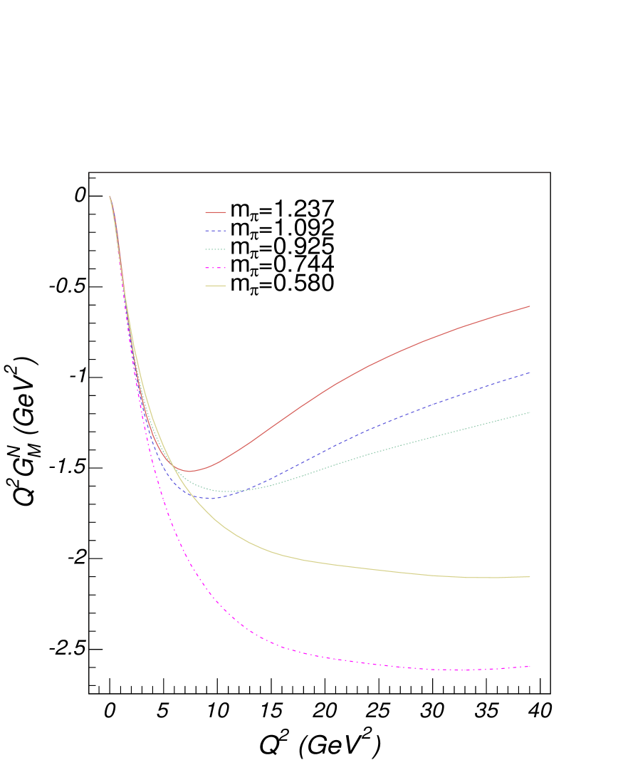
Figure 12: (Color online) LFCBM calculations using parameters (Figs.6, 7 and 8) obtained by fitting the lattice results for the neutron magnetic form factor, $G_{M}$, at lattice  spacing $a=0.26~{}GeV^{-1}$.

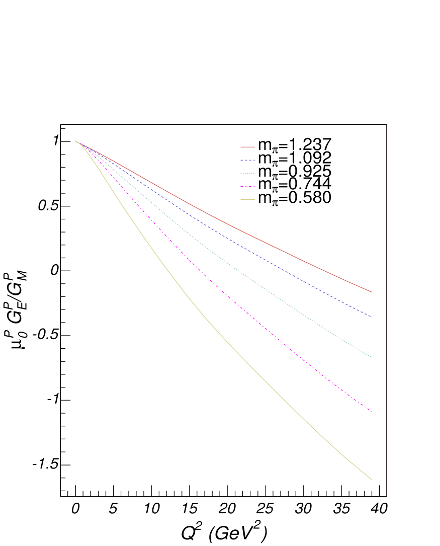
Figure 13: (Color online) LFCBM calculations using parameters (Figs.6, 7 and 8) obtained by reproducing lattice results for the ratio of proton form factors, $\mu_{0}G_{E}/G_{M}$, at lattice  spacing $a=0.26~{}GeV^{-1}$.

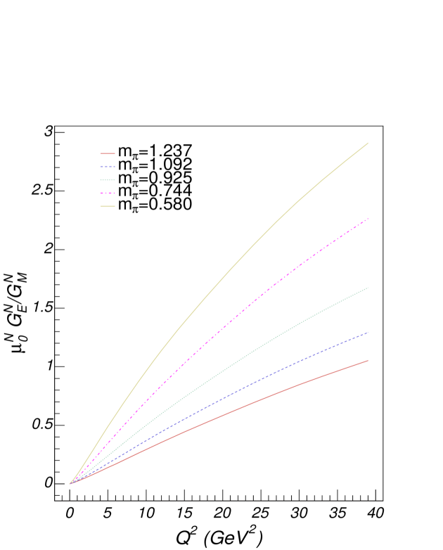
Figure 14: (Color online) LFCBM calculations using parameters (Figs.6, 7 and 8) obtained by reproducing lattice results for the ratio of neutron form factors, $\mu_{0}G_{E}/G_{M}$, at lattice  spacing $a=0.26~{}GeV^{-1}$.

III.3 Results at the Physical Pion Mass and Comparison With Experiment

We use the extrapolated values of $\gamma$ and $M$ (Figs. 6-8) to calculate the nucleon electric and magnetic form factors using the physical pion and nucleon masses. The resulting plots for $G_{E}$, $G_{M}$ and their ratios vs. $Q^{2}$ for both proton and neutron are shown in Figs. 15-20. Figure 17 shows that our results are in more or less good agreement with the experimental data in the low-$Q^{2}$ region, but yield a slightly lower value of $Q^{2}$ for the zero cross-over point than that extrapolated from experiment GE/GM_0_MELNICHUK . A new analysis that includes an estimate of all of the effects of two photon exchange yields a zero-crossing value that is somewhat closer to ours GE/GM-0-CROSS but future data will resolve this unambiguously.

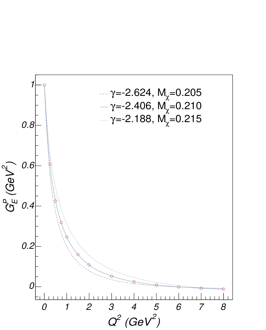
Figure 15: (Color online) Extrapolated calculations for the proton electric form factor, $G_{E}$, for lattice spacing $a=0.26~{}GeV^{-1}$. The dashed and dotted curves show the upper and lower limits of variation of the calculated values due to the uncertainties of the parameters $\gamma$ and $M_{\chi}$.

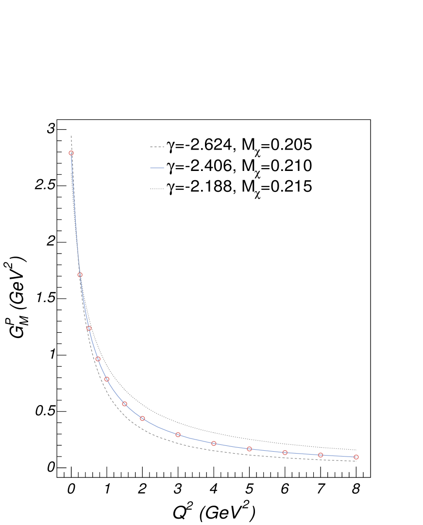
Figure 16: (Color online) Extrapolated calculations for the proton magnetic form factor, $G_{M}$, for lattice spacing $a=0.26~{}GeV^{-1}$. The dashed and dotted curves show the upper and lower limits of variation of the calculated values due to the uncertainties of the parameters $\gamma$ and $M_{\chi}$.

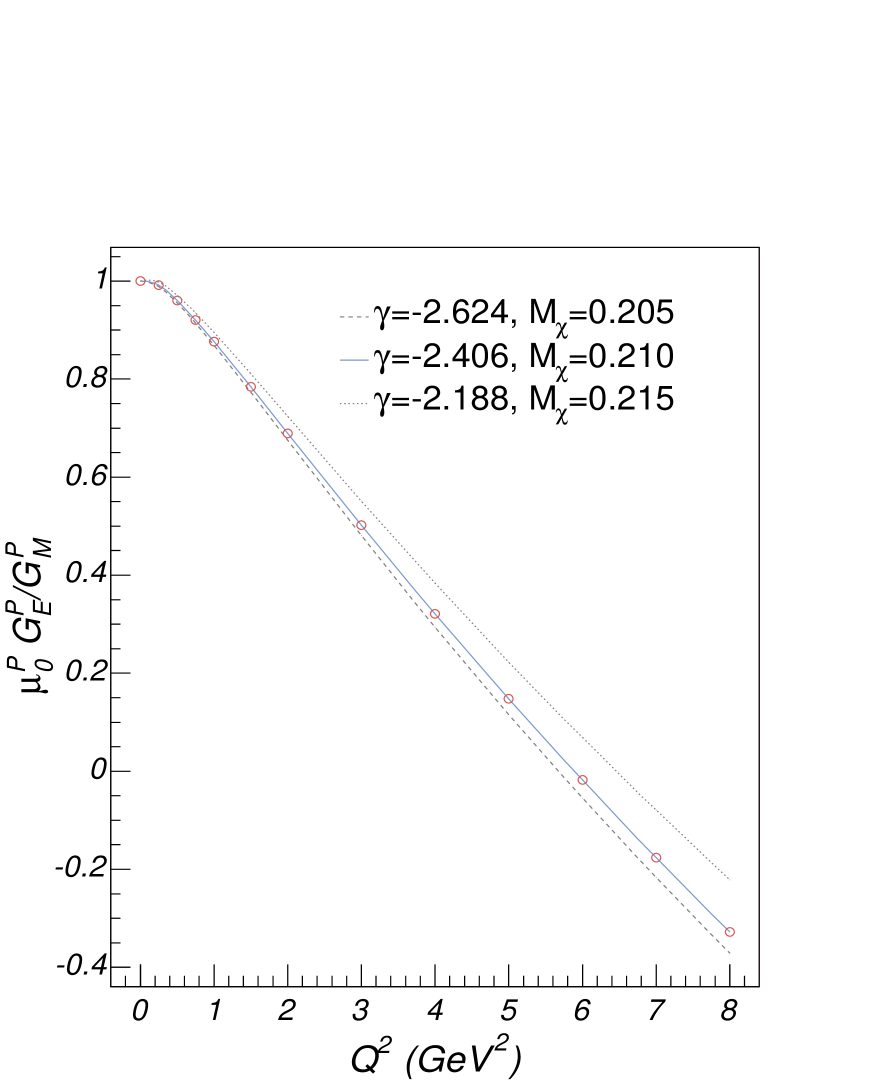
Figure 17: (Color online) Extrapolated calculations for the ratio of proton form factors, $\mu_{0}G_{E}/G_{M}$, for lattice spacing $a=0.26~{}GeV^{-1}$. The dashed and dotted curves show the upper and lower limits of variation of the calculated values due to the uncertainties of the parameters $\gamma$ and $M_{\chi}$.

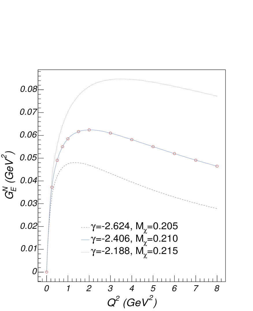
Figure 18: (Color online) Extrapolated calculations for the neutron electric form factor, $G_{E}$, for lattice spacing $a=0.26~{}GeV^{-1}$. The dashed and dotted curves show the upper and lower limits of variation of the calculated values due to the uncertainties of the parameters $\gamma$ and $M_{\chi}$.

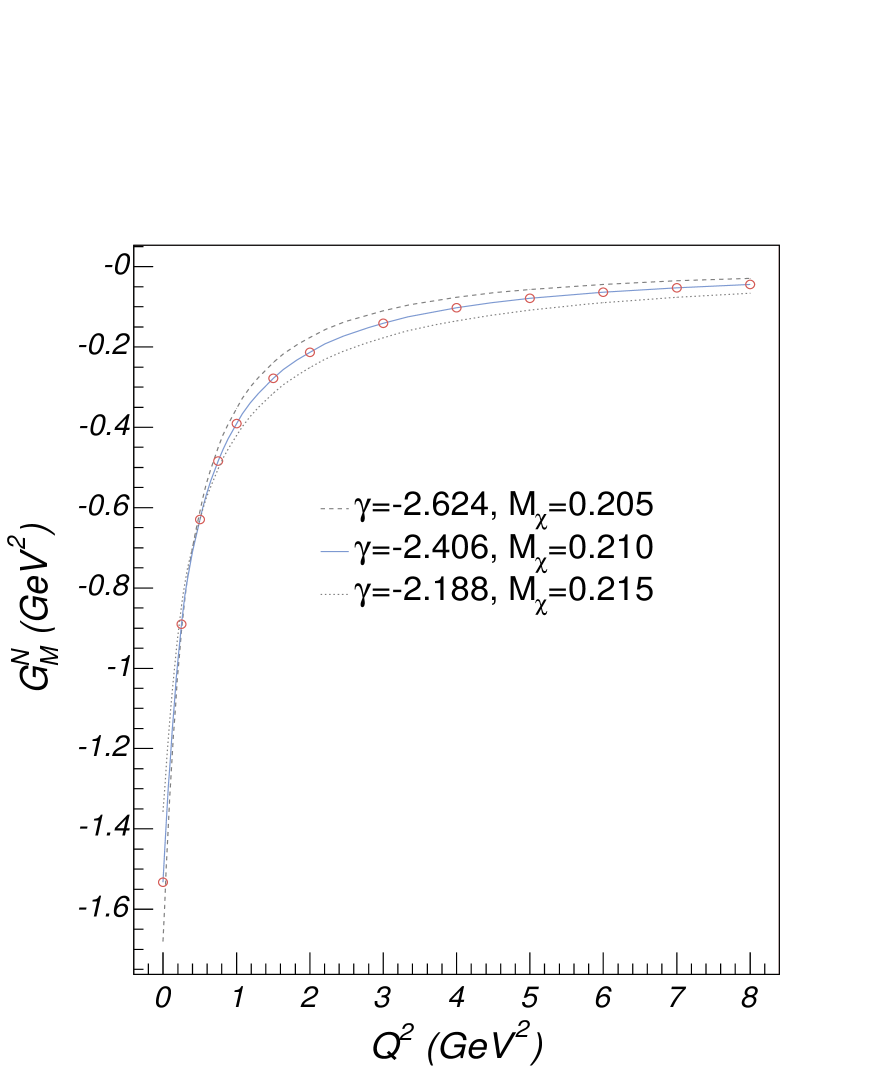
Figure 19: (Color online) Extrapolated calculations for the neutron magnetic form factor,$\ G_{M}$, for lattice spacing $a=0.26~{}GeV^{-1}$. The dashed and dotted curves show the upper and lower limits of variation of the calculated values due to the uncertainties of the parameters $\gamma$ and $M_{\chi}$.

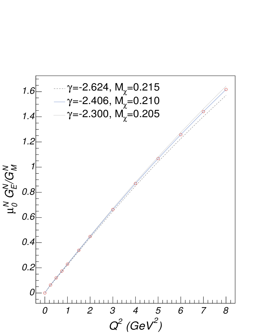
Figure 20: (Color online) Extrapolated calculations for the ratio of neutron form factors, $\mu_{0}G_{E}/G_{M}$, for lattice spacing $a=0.26~{}GeV^{-1}$. The dashed and dotted curves show the upper and lower limits of variation of the calculated values due to the uncertainties of the parameters $\gamma$ and $M_{\chi}$.

An alternative method of determining the value of the $Q^{2}$ for which $G_{E}/G_{M}$ passes through zero at the physical pion mass is to fit the crossover values as a linear function of $m_{\pi}^{2}$ and extrapolate again to the physical pion mass. The resulting plot is shown in Fig. 21.

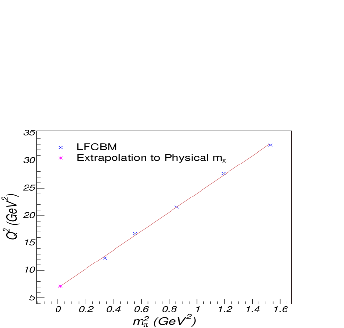
Figure 21: (Color online) Extrapolation of $Q_{Cross}^{2}$ where $G_{E}/G_{M}$ passes through zero for lattice spacing $a=0.26~{}GeV^{-1}$. 

This procedure yields approximately the same cross-over point as found in Fig. 17.

IV Discussion

Our study of the form factors calculated using the LFCBM with parameters determined by lattice data and by extrapolation to the physical pion masses yields very interesting results. The ratio $G_{E}^{p}/G_{M}^{p}$ passes through zero for all of the calculations. The main variation of the position of the crossover between the fitting curves shown in Figs. 13 and 14 comes from the variation of the nucleon mass, and not the variation of $\gamma$. Even though for the physical pion mass, the ratio varies rapidly as a function of $\gamma$ in the region $\gamma\thicksim-2$, the function $G_{E}/G_{M}$ for the neutron has a turning point at about $\gamma\thicksim-2.3$. We shall explain these features using the LFCBM.

Let us express the ratio $G_{E}/G_{M}$ in terms of Pauli and Dirac form factors, $F_{1}$ and $F_{2}$, respectively, using Eq. (3)

$$\frac{G_{E}}{G_{M}}=\frac{F_{1}-Q^{2}/(4M_{N}^{2})F_{2}}{F_{1}+F_{2}}=1-\frac{1+Q^{2}/(4M_{N}^{2})}{1+F_{1}/F_{2}}$$ (15)

Consider first the values of $Q^{2}=(Q^{2}_{\mathrm{Cross}})$ where the ratio $G_{E}/G_{M}$ for the proton passes through zero for the set of calculations shown in Fig. 13. Equation (15) tells us that

$$Q_{\mathrm{Cross}}^{2}=4M_{N}^{2}\frac{F_{1}}{F_{2}}$$ (16)

Now let us consider the formula for $F_{i\alpha}(Q^{2})$, Eq. (7). The second and third terms in Eq. (7) are only significant in the $low-Q^{2}$ region for physical pion masses. In the $high-Q^{2}$ region, or for lattice calculations with high pion mass, these terms are vanishingly small. Indeed the numerical calculations support these statements, so we can neglect their contribution in the rest of the discussion.

The corresponding formulas for $F_{1}^{(0)}$ and $F_{2}^{(0)}$ from Ref. Miller:2002qb are

$$F_{1}^{(0)}(Q^{2})=\int\frac{d^{2}q_{\bot}d\xi}{\xi(1-\xi)}\frac{d^{2}K_{\bot}d\eta}{\eta(1-\eta)}\tilde{\Phi}^{\dagger}(M_{0}^{\prime})\tilde{\Phi}(M_{0})\times\left\langle\chi_{0}^{rel}(\mathbf{p}_{1}^{\prime},\mathbf{p}_{2}^{\prime})|\chi_{0}^{rel}(\mathbf{p}_{1},\mathbf{p}_{2})\right\rangle\left\langle\uparrow\mathbf{p}_{3}^{\prime}|\uparrow\mathbf{p}_{3}\right\rangle$$ (17)

$${\frac{QF_{2}^{(0)}(Q^{2})}{2M_{N}}}=\int\frac{d^{2}q_{\bot}d\xi}{\xi(1-\xi)}\frac{d^{2}K_{\bot}d\eta}{\eta(1-\eta)}\tilde{\Phi}^{\dagger}(M_{0}^{\prime})\tilde{\Phi}(M_{0})\times\left\langle\chi_{0}^{rel}(\mathbf{p}_{1}^{\prime},\mathbf{p}_{2}^{\prime})|\chi_{0}^{rel}(\mathbf{p}_{1},\mathbf{p}_{2})\right\rangle\left\langle\uparrow\mathbf{p}_{3}^{\prime}|\downarrow\mathbf{p}_{3}\right\rangle$$ (18)

The $\tilde{\Phi}(M_{0})$ factors are wave functions of the form of Eq. (5), but using the lattice values of $\gamma,M$ shown in Figs.6-8. We stress that these two integrals differ only by the last factor, which gives the spin non-flip and spin-flip dependence of $F_{1}^{(0)}$ and $QF_{2}^{(0)}/2M_{N}$, respectively. At high $Q^{2}$ these matrix elements are each of order $Q$, causing the ratio $QF_{2}/F_{1}$ to be approximately constant. So we can express $Q_{Cross}^{2}$ as

$$Q_{Cross}^{2}=4M_{N}^{2}\left(\frac{\int\nolimits_{\uparrow\uparrow}}{\int_{\uparrow\downarrow}}\right)^{2}$$ (19)

where $\int\nolimits_{\uparrow\uparrow}$ denotes the integral for $F_{1}^{(0)}$, and $\int_{\uparrow\downarrow}$ denotes the integral for $F_{2}^{(0)}$.

In the high-$Q^{2}$ region the ratio in Eq. (19) is approximately a constant, because the difference comes only from the overlap factors of the spin-dependent parts of the wave functions in the integrals (See Miller:2002ig ,Miller:2003sa ). So the behavior of $Q_{Cross}^{2}$ is governed primarily by the factor $M_{N}^{2}$. The linear variation of $Q_{Cross}^{2}$ vs. $M_{N}^{2}$ presented in Fig. 22 shows the validity of this interpretation.

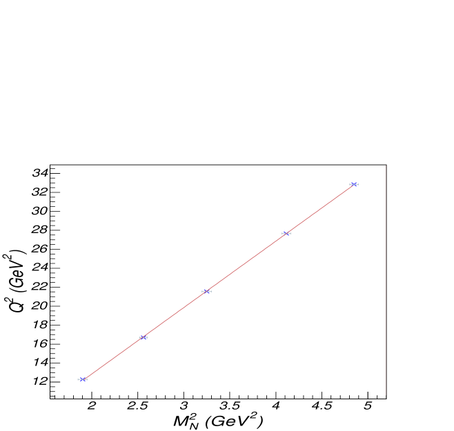
Figure 22: (Color online) Linear fit of $Q_{Cross}^{2}$ where $G_{E}/G_{M}$ passes through zero for lattice spacing $a=0.26~{}GeV^{-1}$. 

We can also understand the behavior of $G_{E}/G_{M}$ versus $\gamma$, by considering its role in the wave function. The factor $\gamma$ determines the size of the momenta appearing in the integrands of Eqs.(17) and (18). The corresponding integrands differ by terms that are ratios of second order polynomials of the integration variables. For large absolute values of $\gamma$, the high momenta are cut off more strongly, so that the contribution of terms that cause differences between the integrals are not very significant. For small absolute values of $\gamma$ the integrals become more sensitive to those terms and we obtain a larger variation of the ratios of the integrals and hence the ratio $G_{E}/G_{M}$.

V Conclusion

We have seen that the LFCBM can produce a very good description of the lattice QCD data for the nucleon form factors over a wide range of quark masses with a smooth, analytic variation of the wave function parameter, $\gamma$, and the constituent quark mass, $M$. The pion cloud plays very little role in the mass range for which the lattice simulations have been made but it rapidly becomes more important as we approach the chiral limit. From the rather strong dependence of the form factors on the lattice spacing, $a$, it is not yet clear that we have obtained a good approximation to the continuum limit, but the form factors obtained at the smallest value of $a$ are in reasonable agreement with experimental data in the low-$Q^{2}$ region for which the lattice simulations were made.

At present the lattice simulations are limited to values of the momentum transfer at or below $2\operatorname{GeV}^{2}$ and it is therefore a very big extrapolation to look at the behavior of the form factors in the region of greatest current interest. Nevertheless, the behavior of $G_{E}/G_{M}$ which we find is particularly interesting. The ratio crosses zero for all values of the quark mass but the position where this happens varies over a very wide range of $Q^{2}$. This variation can be understood almost entirely in terms of the variation of the corresponding nucleon mass, given that the ratio $QF_{1}/F_{2}$ is approximately $Q^{2}$ independent in the model. We obtain the same value of $Q^{2}$ for the cross-over whether we extrapolate the position as a function of quark mass or simply evaluate the form factors at the physical pion mass, using the fitted dependence of the wave function parameters on pion mass.

In the immediate future it is clearly very important to improve on the lattice data, both by ensuring that we really have a good approximation to the continuum limit (e.g., by using a suitably improved action) and by extending the calculations to higher values of $Q^{2}$. It would also be important to remove the need for quenching, even though that may not be such a limitation at large $Q^{2}$. From the point of view of developing a deeper understanding of QCD itself it is important that the LFCBM is able to describe the present lattice data over such a wide range of masses. We would encourage a similar exercise for other models as a novel test of their validity. It remains to be seen whether the LFCBM has indeed been successful in predicting the behavior of the form factors at higher $Q^{2}$ and indeed whether it will match future experimental data.

References

- (1) A. W. Thomas and W. Weise, “The Structure of the Nucleon,” Wiley-VCH, New York (2001)
- (2) T. Reichelt et al. [Jefferson Laboratory E93-038 Collaboration], Eur. Phys. J. A 18, 181 (2003).
- (3) D. I. Glazier et al., arXiv:nucl-ex/0410026.
- (4) J. Friedrich and T. Walcher, Eur. Phys. J. A 17, 607 (2003) [arXiv:hep-ph/0303054].
- (5) A. W. Thomas, Adv. Nucl. Phys. 13, 1 (1984). G. A. Miller, Int. Rev. Nucl. Phys. 2,190 (1984).
- (6) S. Theberge, A. W. Thomas and G. A. Miller, Phys. Rev. D 22, 2838 (1980) [Erratum-ibid. D 23, 2106 (1981)]. A. W. Thomas, S. Theberge and G. A. Miller, Phys. Rev. D 24, 216 (1981). S. Théberge, G. A. Miller and A. W. Thomas, Can. J. Phys. 60, 59 (1982). G. A. Miller, A. W. Thomas and S. Theberge, Phys. Lett. B 91, 192 (1980).
- (7) M. K. Jones et al. [Jefferson Lab Hall A Collaboration], Phys. Rev. Lett. 84, 1398 (2000).
- (8) O. Gayou et al. [Jefferson Lab Hall A Collaboration], Phys. Rev. Lett. 88, 092301 (2002).
- (9) G. A. Miller, Phys. Rev. C 68, 022201 (2003).
- (10) M. R. Frank, B. K. Jennings and G. A. Miller, Phys. Rev. C 54, 920 (1996).
- (11) P. L. Chung and F. Coester, Phys. Rev. D 44, 229 (1991); F. Cardarelli and S. Simula, Phys. Rev. C 62, 065201 (2000); R. F. Wagenbrunn, S. Boffi, W. Klink, W. Plessas and M. Radici, Phys. Lett. B 511, 33 (2001).
- (12) M. Gockeler et al. [QCDSF Collaboration], arXiv:hep-lat/0303019.
- (13) D. B. Leinweber, D. H. Lu and A. W. Thomas, Phys. Rev. D 60, 034014 (1999) [arXiv:hep-lat/9810005].
- (14) E. J. Hackett-Jones, D. B. Leinweber and A. W. Thomas, Phys. Lett. B 489, 143 (2000) [arXiv:hep-lat/0004006].
- (15) T. R. Hemmert and W. Weise, Eur. Phys. J. A 15, 487 (2002) [arXiv:hep-lat/0204005].
- (16) R. D. Young, D. B. Leinweber and A. W. Thomas, Phys. Rev. D71, 014001 (2005); arXiv:hep-lat/0406001.
- (17) J. D. Ashley et al., Eur. Phys. J. A 19, 9 (2004); A. W. Thomas et al., Nucl. Phys. A 721 (2003) 915.
- (18) I. C. Cloet, D. B. Leinweber and A. W. Thomas, Phys. Rev. C 65, 062201 (2002) [arXiv:hep-ph/0203023].
- (19) G. A. Miller, Phys. Rev. C 66, 032201 (2002).
- (20) G. A. Miller and M. R. Frank, Phys. Rev. C 65, 065205 (2002)
- (21) S. J. Brodsky and S. D. Drell, Phys. Rev. D 22, 2236 (1980).
- (22) F. Schlumpf, arXiv:hep-ph/9211255.
- (23) S. J. Chang and T. M. Yan, Phys. Rev. D 7, 1147 (1973).
- (24) V. R. Zoller, Z. Phys. C 53, 443 (1992).
- (25) H. Holtmann, A. Szczurek and J. Speth, Nucl. Phys. A 596, 631 (1996).
- (26) M. A. B. Beg and A. Zepeda, Phys. Rev. D 6, 2912 (1972).
- (27) J. Speth and A. W. Thomas, Adv. Nucl. Phys. 24, 83 (1997).
- (28) D. B. Leinweber et al., Phys. Rev. D 64, 094502 (2001).
- (29) http://root.cern.ch.
- (30) P. G. Blunden, W. Melnitchouk and J. A. Tjon, Phys. Rev. Lett. 91, 142304 (2003); Y. C. Chen et al., Phys. Rev. Lett. 93, 122301 (2004).
- (31) J. Arrington, Phys. Rev. C 68, 034325 (2003) [arXiv:nucl-ex/0305009].