Relativistic Green’s function approach to parity-violating quasielastic electron scattering

Abstract

A relativistic Green’s function approach to parity-violating quasielastic electron scattering is presented. The components of the hadron tensor are expressed in terms of the single particle Green’s function, which is expanded in terms of the eigenfunctions of the non-Hermitian optical potential, in order to account for final state interactions without any loss of flux. Results for ¹²C, ¹⁶O, and ⁴⁰Ca are presented and discussed. The effect of the strange quark contribution to the nuclear current is investigated.

I Introduction

The study of the nucleon with neutral weak probes has recently gained a wide interest in order to investigate the contribution of the sea quarks to ground state nucleon properties, such as spin, charge and magnetic moment kaplan ; beck1 ; beck2 . Besides the measurements of neutrino-nucleus scattering, experiments of parity-violating (PV) electron scattering, combined with existing data of nucleon electromagnetic form factors, may allow to determine possible strange quark contribution to the spin structure of the proton fein ; wale ; mck ; beck ; nap . First measurements of PV asymmetry in elastic electron scattering have been carried out in recent years. The SAMPLE experiment mul at the MIT-Bates Laboratory and the HAPPEX collaboration aniol at Jefferson Laboratory (JLab) investigated such asymmetry at $Q^{2}$ = 0.1 (GeV/c)² and backward direction and 0.5 (GeV/c)² and forward direction, respectively. The first results seemed to indicate a relatively small strangeness contribution to the proton magnetic moment spa ; has and that the strange form factors must rapidly fall off at large $Q^{2}$, if the strangeness radius is large aniol . The HAPPEX2 experiment hap2 at JLab aims at exploring this possibility through an improved measurement at smaller $Q^{2}$. The G0 experiment g0 at JLab plans to measure the scattering of electrons by protons both at backward and forward angles and over the range $0.1\leq Q^{2}\leq 1$ (GeV/c)² in order to investigate the strangeness contribution. The SAMPLE collaboration has recently reported spa2 a new determination of the strange quark contribution to the proton magnetic form factor using a revised analysis of data in combination with the axial form factor of the proton ito . Another measurement of parity violating asymmetry is going on at Mainz Microtron a4 in order to determine the combination of strange Dirac and Pauli form factors at $Q^{2}$ = 0.225 (GeV/c)² with great accuracy. New experiments at JLab he4p plan to measure the parity violating asymmetry using ⁴He and ²⁰⁸Pb as target nuclei. A recent review of the present situation with also a discussion of the theoretical perspectives of this topic can be found in Ref. ram .

In addition to elastic electron scattering, the PV asymmetry can be analyzed in inelastic scattering of polarized electrons on nuclei. Besides the inelastic excitations of discrete states in nuclei mintz , the quasielastic (QE) electron scattering is the most interesting case. In this way, it is possible to understand the role of the various single-nucleon form factors and, by changing the kinematics and the target nucleus, to alter the sensitivity to the various responses. However, nuclear structure effects have to be clearly understood since PV quasielastic electron scattering introduces new complications concerning the nuclear responses to neutral current probes. General review papers about probes of the hadronic weak neutral current can be found in Refs. Walecka ; peccei ; musolf ; amr ; alb ; kolbe03 .

A relativistic mean field model of PV observables and strange-quark contribution was discussed in Ref. horo . The relativistic Fermi gas (RFG) model was applied to investigate the sensitivity to nucleon form factors of parity-conserving (PC) and PV responses in QE scattering from ¹²C in Refs. alb1 ; donnelly , where also strangeness contribution was considered. Different and more complicated models, including correlations and meson-exchange currents were later considered in Refs. alb2 ; barbaro . A continuum shell model description was proposed in Ref. amaro and applied to different closed shell nuclei.

The effect of final state interactions (FSI) has been stressed to significantly contribute to the PC inclusive responses. Namely, it is essential to explain the exclusive one-nucleon knockout, which gives the dominant contribution to the inclusive process in the QE region. It is usually described by an optical potential, whose real component is fitted to elastic proton-nucleus scattering, while the imaginary part takes into account the absorption in the final state. The reaction channels are thus globally described by a loss of flux produced by the imaginary part of the complex potential. This model has been applied with great success to exclusive QE electron scattering book , where it is able to explain the experimental cross sections of one-nucleon knockout reactions in a range of nuclei from ¹²C to ²⁰⁸Pb. In an inclusive process, however, the flux must be conserved. This may be obtained by dropping the imaginary part of the optical potential and neglecting absorption. However, this procedure conserves the flux but it is not consistent with the exclusive reaction, which can only be described with a careful treatment of the optical potential, including both real and imaginary parts book .

We apply a Green’s function approach where the conservation of flux is preserved and FSI are treated in the inclusive reaction consistently with the exclusive one. This method was discussed in a nonrelativistic capuzzi and in a relativistic framework for the case of inclusive PC electron ee and charged-current $\nu$-nucleus cc scattering and it is here applied, in a relativistic framework, to PV electron scattering. In this approach the components of the nuclear response are written in terms of the single-particle optical-model Green’s function. This result can be derived with arguments based on the multiple scattering theory hori , on the Feshbach projection operator formalism capuzzi ; chinn ; bouch ; capma , and on the mass-operator properties kad . Then, the spectral representation of the single-particle Green’s function, based on a biorthogonal expansion in terms of the eigenfunctions of the non-Hermitian optical potential and of its Hermitian conjugate is used to perform explicit calculations and to treat FSI consistently in the inclusive and in the exclusive reactions. Important and peculiar effects are given in the inclusive ($e,e^{\prime}$) reaction by the imaginary part of the optical potential, which is responsible for the redistribution of the strength among different channels.

In Sec. II the general formalism of the PV electron scattering is given. In Sec. III, the Green’s function approach is briefly reviewed. In Sec. IV, the results obtained on ¹²C, ¹⁶O, and ⁴⁰Ca target nuclei are presented and discussed. Some conclusions are drawn in Sec. V.

II Nuclear responses and asymmetry

A polarized electron, with four-momentum $k^{\mu}_{i}=(\varepsilon_{i},\mbox{\boldmath$k$}_{i})$ and longitudinal polarization $\lambda$, is scattered through an angle $\vartheta$ to the final four-momentum $k^{\mu}=(\varepsilon,\mbox{\boldmath$k$})$ via the exchange of a photon or a $Z^{0}$ with the target nucleus with a four-momentum transfer $q^{\mu}=k^{\mu}_{i}-k^{\mu}=(\omega,\mbox{\boldmath$q$})$. The invariant amplitude of the process is given to lowest order by the sum of the one-photon and the one-$Z^{0}$ boson exchange term. The first term is parity-conserving whereas the second one has a parity-violating contribution. The differential cross section is proportional to

$${\rm\,d}\sigma\propto\ \mid\mathcal{M}^{\gamma}+\mathcal{M}^{Z}\mid^{2}\simeq\ \mid\mathcal{M}^{\gamma}\mid^{2}+\ \left(\mathcal{M}^{\gamma}\right)^{\star}\mathcal{M}^{Z}+(\mathcal{M}^{Z})^{\star}\mathcal{M}^{\gamma}\ ,$$ (1)

where the electromagnetic-weak interference term contains the leading order PV contribution, while the very small purely weak term $\mid\mathcal{M}^{Z}\mid^{2}$ can be safely neglected. Eq. 1 can be rearranged to make explicit the contraction between the lepton tensor and the hadron tensor, i.e.,

$${\rm\,d}\sigma_{\lambda}\propto L_{S}^{\mu\nu}W^{\mathrm{S}}_{\mu\nu}+\lambda A_{0}\left[g_{\mathrm{V}}L_{A}^{\mu\nu}W^{\mathrm{I}}_{\mu\nu}(A)+g_{\mathrm{A}}L_{S}^{\mu\nu}W^{\mathrm{I}}_{\mu\nu}(V)\right]\ ,$$ (2)

where the symmetrical and antisymmetrical components, $L_{S}^{\mu\nu}$ and $L_{A}^{\mu\nu}$, of the lepton tensor are defined as in Refs. book ; cc ; nc . $W^{\mathrm{S}}_{\mu\nu}$ is the symmetrical and unpolarized component of the hadron tensor, $W^{\mathrm{I}}_{\mu\nu}(V)$ and $W^{\mathrm{I}}_{\mu\nu}(A)$ are the symmetrical and antisymmetrical polarized components of the hadron tensor, dependent on vector and axial weak currents, respectively. The scale factor $A_{0}$ is defined as

$$A_{0}=\frac{G\ Q^{2}}{2\sqrt{2}\pi\alpha}\simeq 1.798804\times 10^{-4}\frac{Q^{2}}{(\mathrm{GeV/c})^{2}}\ ,$$ (3)

where $G\simeq 1.16639\times 10^{-11}$ MeV^-2 is the Fermi constant, $Q^{2}=\mid\mbox{\boldmath$q$}\mid^{2}-\omega^{2}$, $\alpha$ is the fine structure constant and the couplings $g_{\mathrm{A}}=-1/2$ and $g_{\mathrm{V}}=-1/2+2\sin^{2}{\vartheta_{\mathrm{W}}}\simeq-0.03714$, where $\vartheta_{\mathrm{W}}$ is the Weinberg angle ($\sin^{2}{\vartheta_{\mathrm{W}}}\simeq 0.23143$).

The components of the hadron tensor are given by suitable bilinear products of the transition matrix elements of the nuclear current operator $J^{\mu}$ between the initial state $\mid\Psi_{0}\rangle$ of the nucleus, of energy $E_{0}$, and the final states $\mid\Psi_{\textrm{f}}\rangle$, of energy $E_{\textrm{f}}$, both eigenstates of the $(A+1)$-body Hamiltonian $H$, as

$$W^{\mu\nu}(\omega,q)=\mskip 0.5mu\int\mskip-18.0mu\sum_{\textrm{f}}\langle\Psi_{\textrm{f}}\mid J^{\mu}(\mbox{\boldmath$q$})\mid\Psi_{0}\rangle\langle\Psi_{0}\mid J^{\nu\dagger}(\mbox{\boldmath$q$})\mid\Psi_{\textrm{f}}\rangle\ \delta(E_{0}+\omega-E_{\textrm{f}}).$$ (4)

where the sum runs over all the states of the residual nucleus. The single-particle electromagnetic part of the current is

$$j_{\mathrm{em}}^{\mu}=F_{1}(Q^{2})\gamma^{\mu}+i\frac{\kappa}{2M}F_{2}(Q^{2})\sigma^{\mu\nu}q_{\nu}\ .$$ (5)

The single-particle current operator related to the weak neutral current is

$$j_{\mathrm{nc}}^{\mu}=F_{1}^{\textrm{V}}(Q^{2})\gamma^{\mu}+i\frac{\kappa}{2M}F_{2}^{\textrm{V}}(Q^{2})\sigma^{\mu\nu}q_{\nu}-G_{\textrm{A}}(Q^{2})\gamma^{\mu}\gamma^{5}\ ,$$ (6)

where $\kappa$ is the anomalous part of the magnetic moment and $\sigma^{\mu\nu}=\left(i/2\right)\left[\gamma^{\mu},\gamma^{\nu}\right]$, $F_{1}^{\textrm{V}}$ and $F_{2}^{\textrm{V}}$ are the isovector Dirac and Pauli nucleon form factors, and $G_{\textrm{A}}$ is the axial form factor. The vector form factors $F_{i}^{\mathrm{V}}$ can be expressed in terms of the corresponding electromagnetic form factors for protons $(F_{i}^{\mathrm{p}})$ and neutrons $(F_{i}^{\mathrm{n}})$, plus a possible isoscalar strange-quark contribution $(F_{i}^{\mathrm{s}})$, i.e.,

$$F_{i}^{\mathrm{V}} = \left(\frac{1}{2}-2\sin^{2}{\theta_{\mathrm{W}}}\right)F_{i}^{\mathrm{p}}-\frac{1}{2}F_{i}^{\mathrm{n}}-\frac{1}{2}F_{i}^{\mathrm{s}}\ \ \ \ \ ({\mathrm{proton\ knockout}})\ ,$$

$$F_{i}^{\mathrm{V}} = \left(\frac{1}{2}-2\sin^{2}{\theta_{\mathrm{W}}}\right)F_{i}^{\mathrm{n}}-\frac{1}{2}F_{i}^{\mathrm{p}}-\frac{1}{2}F_{i}^{\mathrm{s}}\ \ \ \ \ ({\mathrm{neutron\ knockout}})\ ,$$ (7)

In the calculations the electromagnetic nucleon form factors are taken from Ref. bba . The strange vector form factors are taken as alb

$$F_{1}^{\mathrm{s}}(Q^{2})=\frac{(\rho^{\mathrm{s}}+\mu^{\mathrm{s}})\tau}{(1+\tau)(1+Q^{2}/M_{\mathrm{V}}^{2})^{2}},\ F_{2}^{\mathrm{s}}(Q^{2})=\frac{\left(\mu^{\mathrm{s}}-\tau\rho^{\mathrm{s}}\right)}{(1+\tau)(1+Q^{2}/M_{\mathrm{V}}^{2})^{2}},$$ (8)

where $\tau=Q^{2}/(4M_{\mathrm{p}}^{2})$ and $M_{\mathrm{V}}$ = 0.843 GeV. The quantities $\mu_{\mathrm{s}}$ and $\rho_{\mathrm{s}}$ are related to the strange magnetic moment and radius of the nucleus.

The axial form factor is expressed as mmd

$$G_{\mathrm{A}} = \frac{1}{2}\left(g_{\mathrm{A}}-g^{\mathrm{s}}_{\mathrm{A}}\right)G\ \ \ \ ({\mathrm{proton\ knockout}})\ ,$$

$$G_{\mathrm{A}} = -\frac{1}{2}\left(g_{\mathrm{A}}+g^{\mathrm{s}}_{\mathrm{A}}\right)G\ \ \ \ ({\mathrm{neutron\ knockout}})\ ,$$ (9)

where $g_{\mathrm{A}}\simeq 1.26$, $g^{\mathrm{s}}_{\mathrm{A}}$ describes possible strange-quark contributions, and

$$G=(1+Q^{2}/M_{\mathrm{A}}^{2})^{-2}.$$ (10)

The axial mass has been taken from Ref. bernard as $M_{\mathrm{A}}$ = (1.026$\pm$0.021) GeV, which is the weighed average of the values obtained from (quasi)elastic neutrino and antineutrino scattering experiments.

One can derive from Eq. 2 the expression for the inclusive differential cross section with respect to the energy and scattering angle of the final electron. The parity-conserving inclusive cross section, for unpolarized electron and considering only the dominant electromagnetic term of the hadron tensor, is

$$\left(\frac{{\rm\,d}\sigma}{{\rm\,d}\varepsilon{\rm\,d}\Omega}\right)^{\mathrm{PC}}=\sigma_{\mathrm{M}}\left[v_{\mathrm{L}}R_{\mathrm{L}}+v_{\mathrm{T}}R_{\mathrm{T}}\right]\ ,$$ (11)

where $\sigma_{\mathrm{M}}$ is the Mott cross section book .

The difference of the polarized cross sections gives the parity-violating contribution, which is obtained from the interference hadron tensor, i.e.,

$$\left(\frac{{\rm\,d}\sigma}{{\rm\,d}\varepsilon{\rm\,d}\Omega}\right)^{\mathrm{PV}} = \frac{1}{2}\left(\frac{{\rm\,d}\sigma_{+}}{{\rm\,d}\varepsilon{\rm\,d}\Omega}-\frac{{\rm\,d}\sigma_{-}}{{\rm\,d}\varepsilon{\rm\,d}\Omega}\right)$$ (12)

$$= \sigma_{\mathrm{M}}A_{0}\Big{[}v_{\mathrm{L}}R_{\mathrm{L}}^{\mathrm{AV}}+v_{\mathrm{T}}R_{\mathrm{T}}^{\mathrm{AV}}+v_{\mathrm{T}}^{\prime}R_{\mathrm{T}}^{\mathrm{VA}}\Big{]},$$

where $A_{0}$ is defined in Eq. 3. The helicity asymmetry can be written as the ratio between the PV and the PC cross section

$$A=A_{0}\frac{v_{\mathrm{L}}R_{\mathrm{L}}^{\mathrm{AV}}+v_{\mathrm{T}}R_{\mathrm{T}}^{\mathrm{AV}}+v_{\mathrm{T}}^{\prime}R_{\mathrm{T}}^{\mathrm{VA}}}{v_{\mathrm{L}}R_{\mathrm{L}}+v_{\mathrm{T}}R_{\mathrm{T}}}\ .$$ (13)

The coefficients $v$ are

$$v_{\mathrm{L}}=\left(\frac{Q^{2}}{|\mbox{\boldmath$q$}|^{2}}\right)^{2}\ ,\ v_{\mathrm{T}}=\tan^{2}\frac{\vartheta}{2}+\frac{Q^{2}}{2|\mbox{\boldmath$q$}|^{2}}\ ,\ v^{\prime}_{\mathrm{T}}=\tan\frac{\vartheta}{2}\left[\tan^{2}\frac{\vartheta}{2}+\frac{Q^{2}}{|\mbox{\boldmath$q$}|^{2}}\right]^{\frac{1}{2}}.$$ (14)

The response functions $R$ are given in terms of the components of the hadron tensor as

$$R_{\mathrm{L}} = W_{00}^{\mathrm{em}}\ ,\ R_{\mathrm{T}}=\left(W_{xx}^{\mathrm{em}}+W_{yy}^{\mathrm{em}}\right)\ ,$$

$$R_{\mathrm{L}}^{\mathrm{AV}} = g_{\mathrm{A}}W_{00}^{\mathrm{I}}\ ,\ R_{\mathrm{T}}^{\mathrm{AV}}=g_{\mathrm{A}}\left(W_{xx}^{\mathrm{I}}+W_{yy}^{\mathrm{I}}\right)\ ,$$

$$R_{\mathrm{T}}^{\mathrm{VA}} = ig_{\mathrm{V}}\left(W_{xy}^{\mathrm{I}}-W_{yx}^{\mathrm{I}}\right)\ ,$$ (15)

where the superscript AV denotes interference of axial-vector leptonic current with vector hadronic current (the reverse for VA).

III The relativistic Green’s function approach

We apply here to the inclusive PV electron scattering the same relativistic approach which was already applied to the inclusive PC electron scattering ee and to the inclusive QE $\nu$($\bar{\nu}$)-nucleus scattering cc . Here we recall only the most important features of the model. More details can be found in Refs. book ; capuzzi ; ee

For the inclusive process the components of the hadron tensor can be expressed as

$$W^{\mu\nu}(\omega,q)=\langle\Psi_{0}\mid J^{\nu\dagger}(\mbox{\boldmath$q$})\delta(E_{\textrm{f}}-H)J^{\mu}(\mbox{\boldmath$q$})\mid\Psi_{0}\rangle\ .$$ (16)

Using the equivalence

$$\delta(E-H)=\frac{1}{2\pi i}[G^{\dagger}(E)-G(E)]\ ,$$ (17)

in terms of the Green’s operators

$$G^{\dagger}(E)=\frac{1}{E-H-i\eta}\ ,\,\,G(E)=\frac{1}{E-H+i\eta}\ ,$$ (18)

related to the nuclear Hamiltonian $H$, we have

$$\omega^{\mu\mu}=W^{\mu\mu}(\omega,q)=-\frac{1}{\pi}\textrm{Im}\langle\Psi_{0}\mid J^{\mu\dagger}(\mbox{\boldmath$q$})G(E_{\textrm{f}})J^{\mu}(\mbox{\boldmath$q$})\mid\Psi_{0}\rangle\ ,$$ (19)

and

$$\omega^{\mu\nu} = W^{\mu\nu}(\omega,q)\pm W^{\nu\mu}(\omega,q)$$ (20)

$$= -\frac{1}{\pi}\textrm{Im}\langle\Psi_{0}\mid J^{\nu\dagger}(\mbox{\boldmath$q$})G(E_{\textrm{f}})J^{\mu}(\mbox{\boldmath$q$})\pm J^{\mu\dagger}(\mbox{\boldmath$q$})G(E_{\textrm{f}})J^{\nu}(\mbox{\boldmath$q$})\mid\Psi_{0}\rangle\ ,$$

for $\mu\not=\nu$, where the upper (lower) sign refers to the symmetrical (antisymmetrical) components of the hadron tensor.

It was shown in Refs. ee ; cc that the nuclear response in Eq. 16 can be written in terms of the single particle Green’s function, $\mbox{$\mathcal{G}$}(E)$, whose self-energy is the Feshbach’s optical potential. A biorthogonal expansion of the full particle-hole Green’s operator is then performed in terms of the eigenfunctions of the non-Hermitian optical potential $\mathcal{V}$ and of its Hermitian conjugate $\mathcal{V}^{\dagger}$,

$$\left[{\mathcal{E}}-T-{\mathcal{V}}^{\dagger}(E)\right]\mid{\chi}_{\mathcal{E}}^{(-)}(E)\rangle=0\ ,\ \ \left[\mathcal{E}-T-{\mathcal{V}}(E)\right]\mid\tilde{\chi}_{\mathcal{E}}^{(-)}(E)\rangle=0\ ,$$ (21)

where $E$ and ${\mathcal{E}}$ are not necessarily the same. The spectral representation of $\mbox{$\mathcal{G}$}(E)$ is

$$\mbox{$\mathcal{G}$}(E)=\int_{M}^{\infty}{\rm\,d}\mathcal{E}\mid\tilde{\chi}_{\mathcal{E}}^{(-)}(E)\rangle\frac{1}{E-\mathcal{E}+i\eta}\langle\chi_{\mathcal{E}}^{(-)}(E)\mid\ .$$ (22)

The hadron tensor components can be reduced to a single-particle expression and $\omega^{\mu\nu}$ can be written in an expanded form as

$$\omega^{\mu\nu}(\omega,q)=-\frac{1}{\pi}\sum_{n}\textrm{Im}\bigg{[}\int_{M}^{\infty}{\rm\,d}\mathcal{E}\frac{1}{E_{{\mathrm{f}}}-\varepsilon_{n}-\mathcal{E}+i\eta}T_{n}^{\mu\nu}(\mathcal{E},E_{{\mathrm{f}}}-\varepsilon_{n})\bigg{]}\ ,$$ (23)

where $n$ denotes the eigenstate $\mid\ n\rangle$ of the residual Hamiltonian of $A$ interacting nucleons related to the discrete eigenvalue $\varepsilon_{n}$. The matrix elements $T^{\mu\nu}$ are defined in terms of the current operators. For the components of $W_{\mathrm{em}}^{\mu\mu}$ we have

$$T_{n,\mathrm{em}}^{\mu\mu}(\mathcal{E},E) = \lambda_{n}\langle\varphi_{n}\mid j_{\mathrm{em}}^{\mu\dagger}(\mbox{\boldmath$q$})\sqrt{1-\mbox{$\mathcal{V}$}^{\prime}(E)}\mid\tilde{\chi}_{\mathcal{E}}^{(-)}(E)\rangle$$ (24)

$$\times \langle\chi_{\mathcal{E}}^{(-)}(E)\mid\sqrt{1-\mbox{$\mathcal{V}$}^{\prime}(E)}j_{\mathrm{em}}^{\mu}(\mbox{\boldmath$q$})\mid\varphi_{n}\rangle\ ,$$

for $\mu=0,x,y$. The components of $W_{\mathrm{I}}^{\mu\mu}$ are

$$T_{n,\mathrm{I}}^{\mu\mu}(\mathcal{E},E) = \lambda_{n}[\langle\varphi_{n}\mid j_{\mathrm{em}}^{\mu\dagger}(\mbox{\boldmath$q$})\sqrt{1-\mbox{$\mathcal{V}$}^{\prime}(E)}\mid\tilde{\chi}_{\mathcal{E}}^{(-)}(E)\rangle$$ (25)

$$\times \langle\chi_{\mathcal{E}}^{(-)}(E)\mid\sqrt{1-\mbox{$\mathcal{V}$}^{\prime}(E)}j_{\mathrm{nc}}^{\mu}(\mbox{\boldmath$q$})\mid\varphi_{n}\rangle$$

$$+ \langle\varphi_{n}\mid j_{\mathrm{nc}}^{\mu\dagger}(\mbox{\boldmath$q$})\sqrt{1-\mbox{$\mathcal{V}$}^{\prime}(E)}\mid\tilde{\chi}_{\mathcal{E}}^{(-)}(E)\rangle$$

$$\times \langle\chi_{\mathcal{E}}^{(-)}(E)\mid\sqrt{1-\mbox{$\mathcal{V}$}^{\prime}(E)}j_{\mathrm{em}}^{\mu}(\mbox{\boldmath$q$})\mid\varphi_{n}\rangle]\ ,$$

for $\mu=0,x,y$, and

$$T_{n,\mathrm{I}}^{xy}(\mathcal{E},E) = \lambda_{n}i[\langle\varphi_{n}\mid j_{\mathrm{em}}^{y\dagger}(\mbox{\boldmath$q$})\sqrt{1-\mbox{$\mathcal{V}$}^{\prime}(E)}\mid\tilde{\chi}_{\mathcal{E}}^{(-)}(E)\rangle$$ (26)

$$\times \langle\chi_{\mathcal{E}}^{(-)}(E)\mid\sqrt{1-\mbox{$\mathcal{V}$}^{\prime}(E)}j_{\mathrm{nc}}^{x}(\mbox{\boldmath$q$})\mid\varphi_{n}\rangle$$

$$- \langle\varphi_{n}\mid j_{\mathrm{em}}^{x\dagger}(\mbox{\boldmath$q$})\sqrt{1-\mbox{$\mathcal{V}$}^{\prime}(E)}\mid\tilde{\chi}_{\mathcal{E}}^{(-)}(E)\rangle$$

$$\times \langle\chi_{\mathcal{E}}^{(-)}(E)\mid\sqrt{1-\mbox{$\mathcal{V}$}^{\prime}(E)}j_{\mathrm{nc}}^{y}(\mbox{\boldmath$q$})\mid\varphi_{n}\rangle$$

$$+ \langle\varphi_{n}\mid j_{\mathrm{nc}}^{y\dagger}(\mbox{\boldmath$q$})\sqrt{1-\mbox{$\mathcal{V}$}^{\prime}(E)}\mid\tilde{\chi}_{\mathcal{E}}^{(-)}(E)\rangle$$

$$\times \langle\chi_{\mathcal{E}}^{(-)}(E)\mid\sqrt{1-\mbox{$\mathcal{V}$}^{\prime}(E)}j_{\mathrm{em}}^{x}(\mbox{\boldmath$q$})\mid\varphi_{n}\rangle$$

$$- \langle\varphi_{n}\mid j_{\mathrm{nc}}^{x\dagger}(\mbox{\boldmath$q$})\sqrt{1-\mbox{$\mathcal{V}$}^{\prime}(E)}\mid\tilde{\chi}_{\mathcal{E}}^{(-)}(E)\rangle$$

$$\times \langle\chi_{\mathcal{E}}^{(-)}(E)\mid\sqrt{1-\mbox{$\mathcal{V}$}^{\prime}(E)}j_{\mathrm{em}}^{y}(\mbox{\boldmath$q$})\mid\varphi_{n}\rangle]\ .$$

The factor $\sqrt{1-\mbox{$\mathcal{V}$}^{\prime}(E)}$ accounts for interference effects between different channels and allows the replacement of the mean field $\mathcal{V}$ by the phenomenological optical potential $\mbox{$\mathcal{V}$}_{\mathrm{L}}$ee . $\lambda_{n}$ is the spectral strength bofficapuzzi of the hole state $\mid\varphi_{n}\rangle$, that is the normalized overlap between $\mid\Psi_{0}\rangle$ and $\mid n\rangle$. After calculating the limit for $\eta\rightarrow+0$, Eq. 23 reads

$$\omega^{\mu\nu}(\omega,q)=\sum_{n}\Bigg{[}\textrm{Re}T_{n}^{\mu\nu}(E_{\mathrm{f}}-\varepsilon_{n},E_{\mathrm{f}}-\varepsilon_{n})$$

$$-\frac{1}{\pi}\mathcal{P}\int_{M}^{\infty}{\rm\,d}\mathcal{E}\frac{1}{E_{\mathrm{f}}-\varepsilon_{n}-\mathcal{E}}\textrm{Im}T_{n}^{\mu\nu}(\mathcal{E},E_{\mathrm{f}}-\varepsilon_{n})\Bigg{]}\ ,$$ (27)

where $\mathcal{P}$ denotes the principal value of the integral.

Disregarding the square root correction, due to interference effects, the second matrix element in Eq. 24, with the inclusion of $\sqrt{\lambda_{n}}$, is the transition amplitude for the single-nucleon knockout from a nucleus in the state $\mid\Psi_{0}\rangle$ leaving the residual nucleus in the state $\mid n\rangle$. The attenuation of its strength, mathematically due to the imaginary part of the optical potential, is related to the flux lost towards the channels different from $n$. In the inclusive response this attenuation must be compensated by a corresponding gain, due to the flux lost, towards the channel $n$, by the other final states asymptotically originated by the channels different from $n$. This compensation is performed by the first matrix element in the right hand side of Eq. 24, where the imaginary part of the potential has the effect of increasing the strength. Similar considerations can be made, on the purely mathematical ground, for the integral of Eq. 27, where the amplitudes involved in $T_{n}^{\mu\nu}$ have no evident physical meaning when ${\mathcal{E}}\neq E_{\rm{f}}-\varepsilon_{n}$.

In an usual shell-model calculation the cross section is obtained from the sum, over all the single-particle shell-model states, of the squared absolute value of the transition matrix elements. Therefore, in such a calculation the negative imaginary part of the optical potential produces a loss of flux that is inconsistent with the inclusive process. In the Green’s function approach the flux is conserved, as the components of the hadron tensor are obtained in terms of the product of the two matrix elements in Eq. 24: the loss of flux, produced by the negative imaginary part of the optical potential in $\chi$, is compensated by the gain of flux produced in the first matrix element by the positive imaginary part of the Hermitian conjugate optical potential in $\tilde{\chi}$.

The cross sections and the response functions are calculated from the single-particle expression of the hadron tensor in Eq. 27. After the replacement of the mean field $\mbox{$\mathcal{V}$}(E)$ by the empirical optical model potential $\mbox{$\mathcal{V}$}_{\textrm{L}}(E)$, the matrix elements of the nuclear current operator in Eqs. 24-26, which represent the main ingredients of the calculation, are of the same kind as those giving the transition amplitudes of the electron induced nucleon knockout reaction in the relativistic distorted wave impulse approximation (RDWIA) meucci1 ; meucci2 .

The relativistic final wave function is written, as in Refs. ee ; meucci1 ; meucci2 ; meucci3 , in terms of its upper component following the direct Pauli reduction scheme, i.e.,

$$\chi_{\mathcal{E}}^{(-)}(E)=\left(\begin{array}[]{c}{\displaystyle\Psi_{\textrm{f}+}}\\ \frac{\displaystyle 1}{\displaystyle M+{\mathcal{E}}+S^{\dagger}(E)-V^{\dagger}(E)}{\displaystyle\mbox{\boldmath$\sigma$}\cdot\mbox{\boldmath$p$}\Psi_{\textrm{f}+}}\end{array}\right)\ ,$$ (30)

where $S(E)$ and $V(E)$ are the scalar and vector energy-dependent components of the relativistic optical potential for a nucleon with energy $E$ chc . The upper component, $\Psi_{\textrm{f}+}$, is related to a two-component spinor, $\Phi_{\textrm{f}}$, which solves a Schrödinger-like equation containing equivalent central and spin-orbit potentials, obtained from the relativistic scalar and vector potentials clark ; HPa , i.e.,

$$\Psi_{\textrm{f}+}=\sqrt{D_{{\mathcal{E}}}^{\dagger}(E)}\ \Phi_{\textrm{f}}\ ,\quad D_{{\mathcal{E}}}(E) = 1+\frac{S(E)-V(E)}{M+{\mathcal{E}}}\ ,$$ (31)

where $D_{{\mathcal{E}}}(E)$ is the Darwin factor.

The wave functions $\varphi_{n}$ are taken as the Dirac-Hartree solutions of a relativistic Lagrangian containing scalar and vector potentials adfx ; lala .

IV Results

The calculations have been performed with the same bound state wave functions and optical potentials as in Refs. ee ; cc ; nc ; meucci1 ; meucci2 ; meucci3 ; rm , where the RDWIA was successfully applied to study $\left(e,e^{\prime}p\right)$, $\left(\gamma,p\right)$, $\left(e,e^{\prime}\right)$ and ($\nu-$nucleus) reactions.

The relativistic bound state wave functions have been obtained as the Dirac-Hartree solutions of a relativistic Lagrangian containing scalar and vector potentials deduced in the context of a relativistic mean field theory that satisfactorily reproduces single-particle properties of several spherical and deformed nuclei adfx ; lala . The scattering state is calculated by means of the energy-dependent and A-dependent EDAD1 complex phenomenological optical potential of Ref. chc , that is fitted to proton elastic scattering data on several nuclei in an energy range up to 1040 MeV.

The initial states $\mid\varphi_{n}\rangle$ are taken as single-particle one-hole states in the target with a unitary spectral strength. The sum runs over all the occupied states.

The results obtained in the Green’s function approach are compared with those given by different approximations in order to show up the effect of the optical potential on the inclusive responses. In the simplest approach the optical potential is neglected, i.e., $\mathcal{V}=\mathcal{V}^{\dagger}=0$ in Eq. 21, and the plane wave approximation (PWIA) is assumed for the final state wave functions ${\chi}^{(-)}$ and $\tilde{\chi}^{(-)}$. In this approximation FSI between the outgoing nucleon and the residual nucleus are completely neglected. In another approach the integrated contribution of all the single-nucleon knockout processes is considered. In this case the negative imaginary part of the optical potential produces a loss of flux that is inconsistent with the inclusive process and results in an underestimation of the responses.

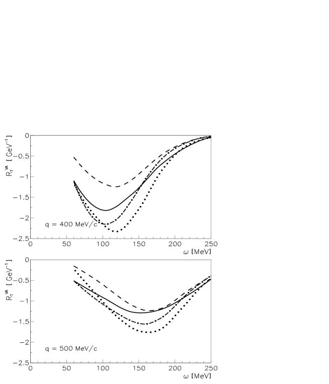
Figure 1: The response function $R_{\mathrm{T}}^{\mathrm{VA}}$ of the ¹²C$(e,e^{\prime})$ reaction for $q$ = 400 and 500 MeV/c. Solid lines represent the result of the Green’s function approach, dotted lines give PWIA, dot-dashed lines show the result without the integral in Eq. 27, and dashed lines the integration of the exclusive reactions with one-nucleon emission.

First, we have considered the ¹²C$(e,e^{\prime})$ reaction at momentum transfer $q$ = 400 and 500 MeV/c. This kinematics corresponds to that of the experiments performed at Saclay saclay . In Fig. 1 our results for the $R_{\mathrm{T}}^{\mathrm{VA}}$ response function are displayed and compared with the other approaches, i.e., PWIA and the integration of all the single-nucleon knockout channels. The PWIA results are generally larger than the Green’s function ones; moreover, a shift of the position of the maximum is visible. The contribution of the single-nucleon emission is smaller than the complete calculation. The difference, that can be attributed to the loss of flux produced by the imaginary part of the optical potential, gives an idea of the relevance of the inelastic channels. In Fig. 1 the results obtained with only the first term of Eq. 27 are also shown. This term can be neglected in a nonrelativistic calculation capuzzi , where it gives only a very small contribution, but must be included in the relativistic approach ee , where it is essential to reproduce the experimental longitudinal response. In accordance with Ref. ee , the contribution of the integral in Eq. 27 gives a 10-15% reduction of the maximum at the momentum transfers considered in Fig. 1 and becomes less important for larger values of the momentum transfer. Similar results are obtained for the $R_{\mathrm{T}}^{\mathrm{AV}}$ and $R_{\mathrm{L}}^{\mathrm{AV}}$ responses, as it can be seen in Figs. 2 and 3. For $R_{\mathrm{L}}^{\mathrm{AV}}$, the PWIA results are smaller than the complete ones. This response function, however, is only a small fraction of the leading response $R_{\mathrm{T}}^{\mathrm{AV}}$ (see also Refs. musolf ; donnelly ). It has been argued barbaro that correlations, which are not included in our calculations, can affect this particular response at low and moderate momentum transfer whereas they mildly influence the other responses.

In Figs. 4, 5, and 6 the same PV responses are shown for the ⁴⁰Ca$(e,e^{\prime})$ reaction at $q$ = 400 and 500 MeV/c. The results are qualitatively similar to those obtained for ¹²C.

In Fig. 7 the PV responses are presented for the ¹⁶O$(e,e^{\prime})$ reaction in a kinematics with beam energies $\varepsilon_{i}$ = 1080 and 1200 MeV and scattering angle $\vartheta$ = 32^o. This choice corresponds to the Frascati kinematics frascati . The Green’s function results are compared with the PWIA ones. In this kinematics at $q$ = 600 MeV/c the contribution of the integral in Eq. 27 is small.

In Figs. 8 and 9 the PV asymmetry of Eq. 13 for ¹²C and ⁴⁰Ca at $q$ = 400 and 500 MeV/c are displayed at four different values of the electron scattering angle. Note that the results are rescaled by the factor $10^{5}$. The asymmetry ranges from a few $\times 10^{-6}$ at forward angle and low momentum transfer to a few $\times 10^{-5}$ at backward angle and greater $q$. The results given by the Green’s function approach are compared with the PWIA ones. Only small differences are found: the Green’s function results are lower in absolute value than the PWIA ones and the shape of the curves is slightly different.

The sensitivity of PV electron scattering to the effect of strange-quark contribution to the vector and axial-vector form factors, is shown in Figs. 10, 11, and 12 for ¹²C at $q$ = 500 MeV/c, $\omega$ = 120 MeV, and $\vartheta$ = 30^o as a function of the strangeness parameters, $\rho^{\mathrm{s}}$, $\mu^{\mathrm{s}}$, and $g^{\mathrm{s}}_{\mathrm{A}}$. The range of their values is chosen according to Refs. beck1 ; aniol . The asymmetry reduces up to 40% as $\rho^{\mathrm{s}}$ varies in the range $-$3 $\leq\rho^{\mathrm{s}}\leq$ $+$3, whereas it changes up to 15% for $-$1 $\leq\mu^{\mathrm{s}}\leq$ $+$1. We note that, according to HAPPEX results aniol , $\rho^{\mathrm{s}}$ and $\mu^{\mathrm{s}}$ might have opposite sign, thus leading to a partial cancellation of the effects. The sensitivity to $g^{\mathrm{s}}_{\mathrm{A}}$ is very weak.

In order to better show up the strangeness effects, in Refs. alb1 ; donnelly ; alb2 ; barbaro ; amaro they were studied through the integrated sum-rule asymmetry:

$$\mathcal{ASR}=\frac{\int{\rm\,d}\omega\left(v_{\mathrm{L}}R_{\mathrm{L}}^{\mathrm{AV}}+v_{\mathrm{T}}R_{\mathrm{T}}^{\mathrm{AV}}+v_{\mathrm{T}}^{\prime}R_{\mathrm{T}}^{\mathrm{VA}}\right)/\tilde{X}_{\mathrm{T}}}{\int{\rm\,d}\omega\left(v_{\mathrm{L}}R_{\mathrm{L}}+v_{\mathrm{T}}R_{\mathrm{T}}\right)/X_{\mathrm{T}}}\ ,$$ (32)

where the functions $\tilde{X}_{\mathrm{T}}$ and $X_{\mathrm{T}}$ are defined in Refs. alb ; barbaro . In Fig. 13 the effect of the strange contribution on the sum-rule asymmetry is shown for the scattering on ¹²C at $q$ = 400 and 500 MeV/c. At forward scattering angle the asymmetry is mainly dependent on the electric strangeness parameter $\rho^{\mathrm{s}}$, whereas the magnetic strangeness parameter $\mu^{\mathrm{s}}$ becomes more important at backward scattering angle. The sensitivity to the strange component of the axial form factor is weaker and only gives, at backward scattering angles, a modest effect that is not shown in the figure. Similar results are obtained when different target nuclei such as ¹⁶O and ⁴⁰Ca are considered.

V Summary and conclusions

A relativistic approach to parity-violating quasielastic electron scattering, based on the spectral representation of the single-particle Green’s function in terms of the eigenfunctions of the complex optical potential and of its Hermitian conjugate, has been presented. This approach has proved to be rather successful in describing inclusive electron scattering and charged-current neutrino-induced reactions. The effects of final state interactions are included in a simple way that keeps flux conservation by using an optical potential consistently with exclusive processes. The imaginary part of the potential accounts for the redistribution of the strength among different channels, without any flux absorption.

The transition matrix elements are calculated using a single-particle model obtained in the framework of the relativistic mean field theory for the structure of the nucleus and applying the direct Pauli reduction for the scattering state.

Calculations of the parity-violating response functions and asymmetry have been presented for ¹²C, ¹⁶O, and ⁴⁰Ca target nuclei and for momentum transfers up to 600 MeV/c. The results of different approximations of final state interactions have been compared. The effect of the optical potential and of the conservation of flux on the response functions is large. Smaller effects are found on the asymmetry. The sensitivity to the strange-quark content of the vector and axial-vector form factors has been investigated with different values of the parameters. Forward-angle scattering may help to determine the electric strangeness whereas backward-angle scattering may add more information about the magnetic strangeness form factor.

Figure 2: The same as in Fig. 1, but for the $R_{\mathrm{T}}^{\mathrm{AV}}$response.

Figure 3: The same as in Fig. 1, but for the $R_{\mathrm{L}}^{\mathrm{AV}}$response.

Figure 4: The response function $R_{\mathrm{T}}^{\mathrm{VA}}$ of the ⁴⁰Ca$(e,e^{\prime})$ reaction for $q$ = 400 and 500 MeV/c. Line convention as in Fig. 1.

Figure 5: The same as in Fig. 4, but for the $R_{\mathrm{T}}^{\mathrm{AV}}$response.

Figure 6: The same as in Fig. 4, but for the $R_{\mathrm{L}}^{\mathrm{AV}}$response.

Figure 7: The response functions $R_{\mathrm{T}}^{\mathrm{VA}}$, $R_{\mathrm{T}}^{\mathrm{AV}}$, and $R_{\mathrm{L}}^{\mathrm{AV}}$ of the ¹⁶O$(e,e^{\prime})$ reaction for $\varepsilon_{i}$ = 1080 (left panels) and 1200 (right panels) MeV and $\vartheta=32^{\mathrm{o}}$. Solid lines represent the result of the Green’s function approach and dotted lines give PWIA.

Figure 8: PV asymmetry for ¹²C at $q$ = 400 and 500 MeV/c. Left panels: PWIA results. Right panels: Green’s function approach. The results are rescaled by the factor $10^{5}$. Solid lines represent the results at $\vartheta$ = 15^o, dashed lines at 45^o, dotted lines at 90^o, and dot-dashed lines at 135^o.

Figure 9: The same as in Fig. 8, but for ⁴⁰Ca$(e,e^{\prime})$ reaction.

Figure 10: PV asymmetry for ¹²C at $q$ = 500 MeV/c, $\omega$ = 120 MeV, and $\vartheta$ = 30^o as a function of $\rho^{\mathrm{s}}$ and $\mu^{\mathrm{s}}$.

Figure 11: The same in Fig. 10, but as a function of $\rho^{\mathrm{s}}$ and $g_{\mathrm{A}}^{\mathrm{s}}$

.

Figure 12: The same in Fig. 10, but as a function of $\mu^{\mathrm{s}}$ and $g_{\mathrm{A}}^{\mathrm{s}}$

.

Figure 13: The sum-rule asymmetry for ¹²C at $q$ = 400 and 500 MeV/c. Solid lines represent the results with no strangeness contribution, dashed (long-dashed) lines with $\mu^{\mathrm{s}}$ = $-$1 (+1), dotted (dot-dashed) lines with $\rho^{\mathrm{s}}$ = $-$3 (+3).

References

- (1) D. Kaplan and A. Manohar, Nucl. Phys. B 310 (1988) 527.
- (2) D.H. Beck and R.D. McKeown, Ann. Rev. Nucl. Part. Sci. 51 (2001) 189.
- (3) D.H. Beck and B.R. Holstein, Int. J. Mod. Phys. E 10 (2001) 1.
- (4) G. Feinberg, Phys. Rev. D 12 (1975) 3575 [Erratum-ibid. D 13 (1976) 2164].
- (5) J.D. Walecka, Nucl. Phys. A 285 (1977) 349.
- (6) R.D. McKeown, Phys. Lett. B 219 (1989) 140.
- (7) D.H. Beck, Phys. Rev. D 39 (1989) 3248.
- (8) J. Napolitano, Phys. Rev. C 43 (1991) 1473.
- (9) B.A. Mueller, et al., Phys. Rev. Lett. 78 (1997) 3824.
- (10) K. Aniol, et al., Phys. Rev. Lett. 82 (1999) 1096; Phys. Rev. C 69 (2004) 065501.
- (11) D.T. Spayde, et al., Phys. Rev. Lett. 84 (2000) 1106.
- (12) R. Hasty, et al., Science 290 (2000) 2117.
- (13) K. Kumar and D. Lhuillier (spokespersons), JLab Experiment 99-115.
- (14) G. Batigne, Eur. Phys. J. A 19-s01 (2004) 207. Additional information can be found at http://www.npl.uiuc.edu/epx/G0.
- (15) D.T. Spayde, et al., Phys. Lett. B 583 (2004) 79.
- (16) T.M. Ito, et al., Phys. Rev. Lett. 92 (2004) 102003.
- (17) D. von Harrach (spokesperson), Mainz Experiment A4; S. Baunack, Eur. Phys. J. A 18 (2003) 159. Additional information can be found at http://www.kph.uni-mainz.de/A4/Welcome.html.
- (18) D.S. Armstrong and R. Michaels (spokespersons), JLab Experiment 00-114; P.Soulder, R. Michaels, and G. Urcioli (spokespersons), JLab Experiment 03-011. Additional information can be found at http://hallaweb.jlab.org/parity/index.html.
- (19) M.J. Ramsey-Musolf, arXiv:nucl-th/0501023.
- (20) S.L. Mintz and M. Pourkaviani, J. Phys. G 18 (1992) 1485.
- (21) J.D. Walecka, in Muon Physics, Vol. II, edited by V.H. Hughes and C.S. Wu (Academic Press, New York, 1975), p. 113.
- (22) T.W. Donnelly and R.D. Peccei, Phys. Rep. 50 (1979) 1.
- (23) M.J. Musolf, T.W. Donnelly, J. Dubach, S.J. Pollock, S. Kowalski, and E.J. Beise, Phys. Rep. 239 (1994) 1.
- (24) J.E. Amaro, M.B. Barbaro, J.A. Caballero, T.W. Donnelly, and A. Molinari, Phys. Rep. 358 (2002) 227.
- (25) W.M. Alberico, S.M. Bilenky, and C. Maieron, Phys. Rep. 368 (2002) 317.
- (26) E. Kolbe, K. Langanke, G. Martinez-Pinedo, and P. Vogel, J. Phys. G 29 (2003) 2569.
- (27) C. J. Horowitz, Phys. Rev. C 47 (1993) 826.
- (28) W.M. Alberico, T.W. Donnelly, and A. Molinari, Nucl. Phys. A 512 (1990) 541.
- (29) T.W. Donnelly, M.J. Musolf, W.M. Alberico, M.B. Barbaro, A. De Pace, and A. Molinari, Nucl. Phys. A 541 (1992) 525.
- (30) W.M. Alberico, M.B. Barbaro, A. De Pace, T.W. Donnelly, and A. Molinari, Nucl. Phys. A 563 (1993) 605.
- (31) M.B. Barbaro, A. De Pace, T.W. Donnelly, and A. Molinari, Nucl. Phys. A 569 (1994) 701.
- (32) J.E. Amaro, J.A. Caballero, T.W. Donnelly, A. Lallena, E. Moya de Guerra, and J.M. Udías, Nucl. Phys. A 602 (1996) 263.
- (33) S. Boffi, C. Giusti, F.D. Pacati, and M. Radici, Electromagnetic Response of Atomic Nuclei, Oxford Studies in Nuclear Physics, Vol. 20 (Clarendon Press, Oxford, 1996); S. Boffi, C. Giusti, and F.D. Pacati, Phys. Rep. 226 (1993) 1.
- (34) F. Capuzzi, C. Giusti, and F.D. Pacati, Nucl. Phys. A 524 (1991) 681.
- (35) A. Meucci, F. Capuzzi, C. Giusti, and F.D. Pacati, Phys. Rev. C 67 (2003) 054601.
- (36) A. Meucci, C. Giusti, and F.D. Pacati, Nucl. Phys. A 739 (2004) 277.
- (37) Y. Horikawa, F. Lenz, and N.C. Mukhopadhyay, Phys. Rev. C 22 (1980) 1680.
- (38) C.R. Chinn, A. Picklesimer, and J.W. Van Orden, Phys. Rev. C 40 (1989) 790; 40 (1989) 1159.
- (39) P.M. Boucher and J.W. Van Orden, Phys. Rev. C 43 (1991) 582.
- (40) F. Capuzzi and C. Mahaux, Ann. Phys. (N.Y.) 254 (1997) 130.
- (41) F. Capuzzi, C. Giusti, F.D. Pacati, and D.N. Kadrev, Ann. Phys. (N.Y.) (2005) in press.
- (42) A. Meucci, C. Giusti, and F.D. Pacati, Nucl. Phys. A 744 (2004) 307.
- (43) H. Budd, A. Bodek, and J. Arrington, arXiv:hep-ex/0308005.
- (44) M.J. Musolf and T.W. Donnelly, Nucl. Phys. A 546 (1992) 509.
- (45) V. Bernard, L. Elouadrhiri, and Ulf-G. Meissner, J. Phys. G 28 (2002) R1.
- (46) S. Boffi and F. Capuzzi, Nucl. Phys. A 351 (1981) 219.
- (47) A. Meucci, C. Giusti, and F.D. Pacati, Phys. Rev. C 64 (2001) 014604.
- (48) A. Meucci, C. Giusti, and F.D. Pacati, Phys. Rev. C 64 (2001) 064615.
- (49) A. Meucci, Phys. Rev. C 65 (2002) 044601.
- (50) E.D. Cooper, S. Hama, B.C. Clark, and R.L. Mercer, Phys. Rev. C 47 (1993) 297.
- (51) B.C. Clark, in Proceedings of the Workshop on Relativistic Dynamics and Quark-Nuclear Physics, edited by M.B. Johnson and A. Picklesimer (John Wiley & Sons, New York, 1986), p. 302.
- (52) M. Hedayati-Poor, J.I. Johansson, and H.S. Sherif, Nucl. Phys. A 593 (1995) 377.
- (53) W. Pöschl, D. Vretenar, and P. Ring, Comput. Phys. Commun. 103 (1997) 217.
- (54) G.A. Lalazissis, J. König, and P. Ring, Phys. Rev. C 55 (1997) 540.
- (55) M. Radici, A. Meucci, and W.H. Dickhoff, Eur. Phys. J. A 17 (2003) 65.
- (56) P. Barreau, et al., Nucl. Phys. A 402 (1983) 515; CEA Report No. N-2334.
- (57) M. Anghinolfi, et al., Nucl. Phys. A 602 (1996) 405.
.
.