Effective Interaction Techniques for the Gamow Shell Model

Abstract

We apply a contour deformation technique in momentum space to the newly developed Gamow shell model, and study the drip-line nuclei ⁵He, ⁶He and ⁷He. A major problem in Gamow shell-model studies of nuclear many-body systems is the increasing dimensionality of many-body configurations due to the large number of resonant and complex continuum states necessary to reproduce bound and resonant state energies. We address this problem using two different effective operator approaches generalized to the complex momentum plane. These are the Lee-Suzuki similarity transformation method for complex interactions and the multi-reference perturbation theory method. The combination of these two approaches results in a large truncation of the relevant configurations compared with direct diagonalization. This offers interesting perspectives for studies of weakly bound systems.

I Introduction

We expect that present and proposed nuclear structure research facilities for radioactive beams will open new territory into regions of heavier nuclei. Such systems pose significant challenges to existing nuclear structure models since many of these nuclei will be unstable and short-lived. How to deal with weakly bound systems and coupling to resonant states is an open and interesting problem in nuclear spectroscopy. Weakly bound systems cannot be properly described within a standard shell-model approach since even bound states exhibit a strong coupling with the continuum.

It is therefore important to investigate theoretical methods that will allow for a description of systems involved in such element production. Ideally, we would like to start from an ab initio approach with the free nucleon-nucleon interaction and eventually also three-body interactions as the basic building blocks for the derivation of an effective shell-model interaction. The newly developed Gamow shell model offers such a possibility, see for example Refs. michel1 ; michel2 ; michel3 ; liotta ; betan ; witek1 ; witek2 ; roberto ; betan2 . Similarly, the recent work on the continuum shell-model by Volya and Zelevinsky vz2003 conveys similar interesting prospectives. Here we focus on the Gamow shell model, which has proved to be a powerful tool in describing and understanding the formation of multi-particle resonances within a shell-model formulation. Representing the shell-model equations using a Berggren basis berggren ; berggren1 ; berggren2 ; berggren3 ; lind ; hagen , allows for a simple interpretation of multi-particle resonances in terms of single-particle resonances, as opposed to the traditional harmonic oscillator representation, where resonances never appear explicitly.

Although the Gamow shell-model approach is a powerful tool in this respect, there are major computational and theoretical challenges that need to be overcome if we aim at a realistic description of weakly bound and unbound nuclei. One of the challenges regarding the Gamow shell model discussed in Refs. liotta ; betan , was the problem of choosing a contour in the complex $k$-plane that in the many-particle case selects the physical interesting states from the dense distribution of continuum states. In Refs. liotta ; betan the authors employ a “square-well” contour, which in the two-particle case separates the resonances from the complex-continuum states. In the case where more than two particles are present in the shell-model space, the resonant states mix with the complex continuum states, and an identification of the multi-particle resonances becomes difficult.

In this work we consider as a test case the light drip-line nuclei ^5,6,7He, and the formation of resonances in these nuclei starting from a single-particle picture. These nuclei have also been studied with a number of other methods, see for example Ref. jonson , and references therein. We construct a single-particle basis using the contour deformation method in momentum space, discussed in detail in Ref. hagen , see also Ref. nimrod for further references on complex scaling. We show that choosing a rotated plus translated contour in the complex plane, a large portion of the many-particle energy surface is free from complex continuum states. This choice of contour isolates the physical resonances, and allows for a clear distinction of many-particle resonances from the dense distribution of complex continuum states, also in the case when the number of particles exceeds two.

The most severe problem and future challenge is that the shell-model dimension increases dramatically for $n>2$ particles moving in a large valence space, this is what we henceforth refer to as the dimensionality problem. Using a technique such as the traditional Lanczos iteration method lanczo fails in Gamow shell-model calculations. Dealing with large real symmetric matrices, the Lanczos scheme is a powerful method when one wishes to calculate the states lowest in energy. In Gamow shell-model calculations there may be a large number of complex continuum states lying below the physical resonances in real energy. In addition it is difficult to predict where the multi-particle resonances will appear after diagonalization. In Refs. witek1 ; witek2 this problem was circumvented by choosing a small number of complex continuum states in the single-particle basis. It was also pointed out that the results obtained were not converged with respect to the number of single-particle continuum orbits. In Ref. michel2 another approach was considered, where at most two particles where allowed to move in complex continuum states. This was based on the assumption that these configurations play the dominant role in the formation of many-particle resonances, and configurations where more than two particles move in continuum states could be neglected.

Our aim in this work is to propose an effective interaction scheme which allows for a much larger number of complex continuum states in the calculations, and in addition takes into account the mixing of configurations where all particles may move in complex continuum states. We show that if one aims at accurate calculations of the multi-particle resonances, the effect of all particles moving in the continuum may not always be neglected. Our choice of contour allows for a perturbative treatment of the many-particle resonances, and we propose a perturbation theory based scheme which combines the Lee-Suzuki similarity transformation method suzuki1 ; suzuki2 ; suzuki3 ; suzuki4 and the so-called multi-reference perturbation method multi1 ; multi2 ; multi3 to account for couplings with configurations where all single-particles move in complex continuum states.

Presently, Gamow shell-model calculations have been performed with phenomenological nucleon-nucleon interactions. A major challenge is to construct effective nucleon-nucleon interactions for drip-line nuclei starting from a realistic nucleon-nucleon interaction. In this paper we focus on the choice of contour and the dimensionality problem. The effective nucleon-nucleon interaction adopted is purely phenomenological. However, the scheme we present, although implemented with a phenomenological nucleon-nucleon interaction, allows to define effective interactions computed with the complex scaled single-particle basis. The problem of constructing an effective interaction based on present interaction models for the nucleon-nucleon force will be considered in a forthcoming work.

The outline of this work is as follows. Sec. II gives a brief description of the contour deformation method in momentum space, and presents calculations of the energy spectrum of the nuclei ^5,6,7He. Sec. III presents first the Lee-Suzuki transformation method generalized to complex interactions. Thereafter we apply the similarity transformation method to the unbound nucleus ⁷He and give a convergence study of its $J^{\pi}=3/2^{-}_{1}$ ground state resonance. Sec. IV gives a brief outline of the multi-reference perturbation method, and its application to the ground state of ⁷He. In Sec. V we present an effective interaction scheme, which combines the Lee-Suzuki similarity transformation and the multi-reference perturbation method, for calculation of multi-particle resonances in weakly bound nuclei. Sec. VI gives the conclusions of the present study and future perspectives and challenges for Gamow shell-model calculations.

II The Gamow Shell Model

The newly developed Gamow shell model has proved to be a powerful tool in describing and understanding multi-particle resonances appearing in nuclei near the drip-lines. Here we discuss how two- and three-particle resonances are formed in ⁶He and ⁷He, and how they are to be understood in terms of a single-particle picture. The specific choice of contour in the complex $k$-plane makes it easy to identify and interpret the multi-particle resonances. In this section no truncations are made, all possible configurations within a model space are used in the shell model calculations.

II.1 Berggren Basis in the Momentum Representation

In Ref. hagen we studied the contour deformation method applied to the momentum space Schrödinger equation. It was discussed and shown how the specific choices of contours based on the analytic structure of the potential may allow for a unified description of bound, anti-bound (virtual) and resonant states. We will apply this method to obtain a single-particle Berggren basis for use in Gamow shell-model calculations. Here we briefly outline the contour deformation method, and refer the reader to Ref. hagen for a more rigorous discussion.

The analytically continued Schrödinger equation on a general inversion symmetric contour takes the form

$${\hbar^{2}\over 2\mu}k^{2}\psi_{nl}(k)+{2\over\pi}\int_{C^{+}}dq{q}^{2}V_{l}(k,q)\psi_{nl}(q)=E_{nl}\psi_{nl}(k).$$ (1)

Here both $k$ and $q$ are defined on an inversion symmetric contour $C^{+}$ in the lower half complex $k$-plane, resulting in a closed integral equation. The eigenfunctions constitute a complete bi-orthogonal set, normalized according to the Berggren metric berggren ; berggren1 ; berggren2 ; berggren3 ; lind , namely

$${\bf 1}=\sum_{n\in\bf{C}}|\psi_{nl}\rangle\langle\psi_{nl}^{*}|+\int_{C^{+}}dkk^{2}|\psi_{l}(k)\rangle\langle\psi_{l}^{*}(k)|.$$ (2)

In this work we construct a single-particle Berggren ensemble on a rotated plus translated contour, $C_{R+T}$, in the complex $k$-plane, studied in detail in Ref. hagen . The contour $C_{R+T}^{+}$ is part of the inversion symmetric contour $C_{R+T}=C_{R+T}^{+}+C_{R+T}^{-}$ displayed in Fig. 1.

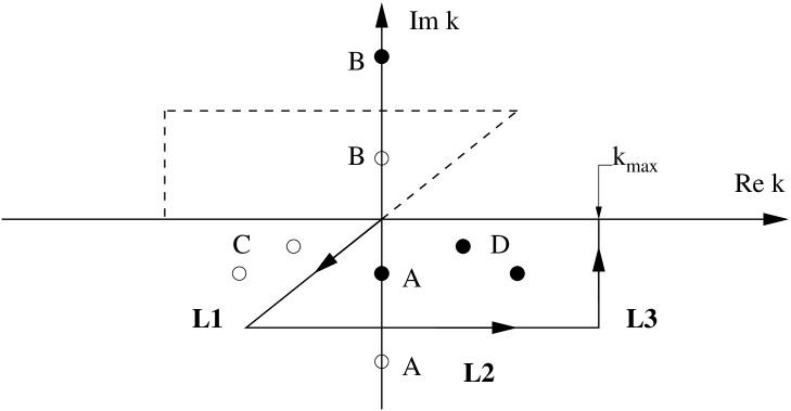
Figure 1: Contour $C_{R+T}^{+}=L_{1}+L_{2}+L_{3}$ is given by the solid line, while the contour $C_{R+T}^{-}$ is given by the dashed line. The contour $C_{R+T}=C_{R+T}^{+}+C_{R+T}^{-}$ is inversion symmetric. The single-particle spectrum which is exposed by this contour is marked by filled circles $\bullet$ and the excluded spectrum by open circles $\circ$. The full spectrum includes bound states (B), anti-bound (A), decay (D) and capture (C) resonant states.

The complete set of single-particle orbits defined by this contour will then include anti-bound, bound and resonant states. This basis serves as our starting point for Gamow shell-model calculations.

II.2 Single-Particle Spectrum of ⁵He

We consider first the unbound nucleus ⁵He. This nucleus may be modeled by an inert ⁴He core with a neutron moving mainly in the resonant spin-orbit partners $p_{3/2}$ and $p_{1/2}$. The $J^{\pi}={3/2^{-}_{1}}$ resonance, to be associated with the single-particle orbit $p_{3/2}$, is experimentally known to have a width of $\Gamma\approx 0.60$ MeV while the $J^{\pi}={1/2^{-}_{1}}$ resonance, associated with the single-particle orbit $p_{1/2}$, has a large width $\Gamma\approx 4$ MeV. For more information on these systems, see for example the recent review by Jonson jonson . The core-neutron interaction in ⁵He may be phenomenologically modeled by the SBB (Sack, Biedenharn and Breit) potential  SBB . The SBB potential is of Gaussian type with a spin-orbit term, fitted to reproduce the neutron - ⁴He scattering phase shifts. In momentum space the SBB potential, which consist of a central part $c$ and a spin-orbit term $\vec{\sigma}\vec{l}$, reads

$$V_{lj}(k,k^{\prime})=V_{lj}^{c}(k,k^{\prime})+({\vec{\sigma}\cdot\vec{{l}}}\>)V_{lj}^{\sigma l}(k,k^{\prime}),$$ (3)

with

$$V_{l,j}^{i}(k,k^{\prime})=-g_{i}{\pi\over 4\alpha^{2}_{i}}{1\over\sqrt{kk^{\prime}}}\exp({-\left({k^{2}+{k^{\prime}}^{2}\over 4\alpha^{2}_{i}}\right)})I_{l+1/2}\left({kk^{\prime}\over 2\alpha^{2}_{i}}\right),$$ (4)

where the subscripts $lj$ refer to the single-particle orbital and angular momentum quantum numbers $l$ and $j$, respectively. The term $I_{l+1/2}(z)$ is a Bessel function of the first kind with complex arguments. Fitting this potential to reproduce the ⁵He single-particle spectrum and phase-shifts results in $g_{c}=47.4$ MeV, $g_{\sigma l}=5.86$ MeV and $\alpha_{c}=\alpha_{\sigma l}=2.3$ fm^-1.

In the complex $k$-plane the Gaussian potential diverges exponentially for $|\mathrm{Im}[k]|>|\mathrm{Re}[k]|$. If we apply the complex scaling technique, which consists of solving the momentum space Schrödinger equation on a purely rotated contour, we get the restriction $\theta<\pi/4$ on the rotation angle. Even for smaller angles we may get a poor convergence, since the Gaussian potential oscillates strongly along the rotated contours. On the other hand, choosing a contour of the type $C_{R+T}^{+}$ solves this problem, allowing for a continuation in the third quadrant of the complex $k$-plane. Furthermore, it yields a faster and smoother decay of the Gaussian potential along the chosen contour.

Since ⁵He has only resonances in its spectrum, viz., no anti-bound states, there is no need for an analytic continuation in the third quadrant of the complex $k$-plane, as done in Ref. hagen for the free nucleon-nucleon interaction. We choose a contour of the type $C^{+}_{R+T}$ rotated with $\theta=\pi/4$ and translated with $|\mathrm{Im}[k]|=0.4\sin(\pi/4)\approx 0.28$ fm^-1 in the fourth quadrant of the complex $k$-plane. Figs. 2 and 3 give plots of the single-particle spectrum in ⁵He for the spin-orbit partners $p_{3/2}$ and $p_{1/2}$ respectively. We have used 50 integration points along the rotated $C_{R}$, and the translated $C_{T}$ parts of the contour $C^{+}_{R+T}$ in the complex $k$-plane.

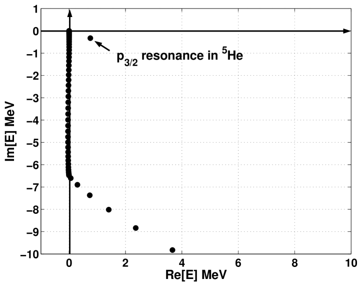
Figure 2: Plot of the $p_{3/2}$ single-particle spectrum in ⁵He for a Gaussian single-particle potential. The resonance is well located. The remaining points represent the non-resonant continuum.

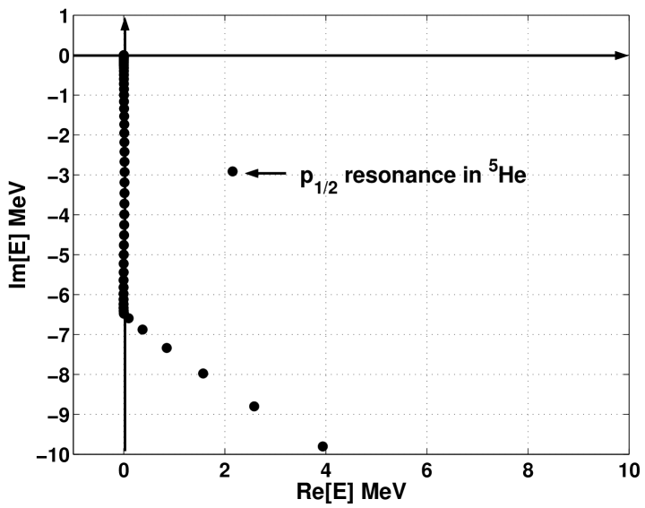
Figure 3: Plot of the $p_{1/2}$ single-particle spectrum in ⁵He for a Gaussian single-particle potential. The resonance is well located. The remaining points represent the non-resonant continuum.

Table 1 gives the convergence of the $p_{3/2}$ and the $p_{1/2}$ single-particle resonances as function of integration points along the contour $C_{R+T}$. We observe that with $12$ points along the rotated path and $12$ points along the translated line, one has a reasonable convergence of the resonance energy, giving in total $48$ single-particle states for the valence space consisting of the $lj$ orbits $\{p_{3/2},p_{1/2}\}$ with their pertinent momenta $k$ defined by the number of mesh points. It is clear that if several particles were to move in this space, the dimensionality would become enormous. It is therefore important, even at the single-particle stage, to optimize the distribution of continuum states, in order that the main features of the system are reproduced with a small number of single-particle resonances and complex continuum states.

Table 1: Convergence of $p_{3/2}$ and $p_{1/2}$ resonance energies in ⁵He as function of the number of integration points $N_{R}$ along the rotated $C_{R}$ and $N_{T}$ along the translated part $C_{T}$ of the contour. Energies are given in units of MeV.

		$J^{\pi}={3/2}^{-}$		$J^{\pi}={1/2}^{-}$
$N_{R}$	$N_{T}$	Re[E]	Im[E]	Re[E]	Im[E]
10	10	0.752321	-0.329830	2.148476	-2.912522
12	12	0.752495	-0.327963	2.152992	-2.913609
20	20	0.752476	-0.328033	2.154139	-2.912148
30	30	0.752476	-0.328033	2.154147	-2.912162
40	40	0.752476	-0.328033	2.154147	-2.912162

Notice also that the calculated width of the ${1/2}^{-}$ resonance is somewhat larger ($\approx 6$ MeV) than the experimental value ($\approx 4$ MeV), see Ref. jonson .

II.3 Two-Particle Resonances in ⁶He

Here we present results for the resonant spectra of ⁶He. We employ again a shell-model picture with ⁶He modeled by an inert ⁴He core and two valence neutrons moving in the $lj$ orbits $\{p_{3/2},p_{1/2}\}$, ignoring the recoil from the core. The model space consists then of all momenta $k$ defined by the set of mesh points along the various contours, pertinent to these two $lj$ orbits. Using the single-particle wave functions for ⁵He of Subsec II.2, we can in turn construct an anti-symmetric two-body wave function based on these single-particle wave functions, viz.,

$$\Psi_{\alpha}^{JM}(1,2)=\sum_{a\leq b}C_{a,b}^{JM}{\Phi}_{a,b}^{JM}(1,2),$$ (5)

where the indices $a,b$ represent the various single-particle orbits. Here ${\Phi}_{a,b}^{J}(1,2)$ is an anti-symmetric two-particle basis state in the $j-j$ coupling scheme. The sum over single-particle orbits is limited by $a\leq b$ since we deal with identical particles only. The expansion coefficients fulfill the completeness relation

$$1=\sum_{a\leq b}\left(C_{a,b}^{JM}\right)^{2},$$ (6)

and the two-particle Berggren basis forms a complete set

$$1=\sum_{a\leq b}|{\Phi}_{a,b}^{JM}(1,2)\rangle\langle\tilde{\Phi}_{a,b}^{JM}(1,2)|.$$ (7)

Here $\langle\tilde{\Phi}_{a,b}^{JM}(1,2)|$ is the complex conjugate of $\langle{\Phi}_{a,b}^{JM}(1,2)|$. As an effective two-neutron interaction $V_{ij}$ we use a phenomenological interaction of Gaussian type, separable in $\bf{r}_{i},\bf{r}_{j}$, given by

$$V_{ij}({\bf{r}_{i},\bf{r}_{j}})=V_{0}\exp(-\alpha^{2}(r_{i}^{2}+r_{j}^{2}))\sum_{\lambda}(Y_{\lambda}(i)\cdot Y_{\lambda}(j)).$$ (8)

Two model spaces were considered. The first case includes only the $p_{3/2}$ single-particle orbit for various values of the momentum $k$ to be defined below. The second model space includes also the $p_{1/2}$ single-particle orbit and its relevant momenta. For both model spaces we fit the interaction strength to reproduce the $0^{+}$ binding energy in ⁶He. We have observed that the position of the $2^{+}$ resonance in ⁶He depends on the range $\alpha$ of the Gaussian interaction, even though the $0^{+}$ ground state does not change with $\alpha$. Unfortunately it turns out that for larger values of $\alpha$ the energy fit is better, but the convergence as function of meshpoints is poorer. In our calculations we have chosen a value of $\alpha$ which is a compromise between a small number of mesh points along the contour and a reasonable good fit of the resonant energy spectra. This demonstrates that the two-particle resonant spectrum depends on the radial shape of the interaction and suggests that we should rather deal with an effective interaction derived from realistic models for the nucleon-nucleon interaction. The parameters used in our calculations are $V_{0}=-5.315$ MeV for the model space involving only the $(p_{3/2})$ states and $V_{0}=-4.549$ MeV for a model space consisting of both single-particle quantum states $p_{3/2}$ and $p_{1/2}$. We use $\alpha=4.8$ fm^-1 for both model spaces.

Figs. 4 and 5 show the $0^{+}$ and $2^{+}$ energy spectrum, respectively, for ⁶He after a full diagonalization of the two-particle shell-model equation. Here the model space is defined by the $p_{3/2}$ and $p_{1/2}$ single-particle orbits. This model space yields a bound $0^{+}$ state as well as a resonant $0^{+}$ state. Moreover, we obtain two resonant $2^{+}$ states. Observe that the choice of contour ($C^{+}_{R+T}$) separates all physical relevant states from the dense distribution of complex continuum states in the energy plane. By this choice of contour the identification of multi-particle resonances is fairly easy, and one may study the resonant trajectories as the interaction strength is varied.

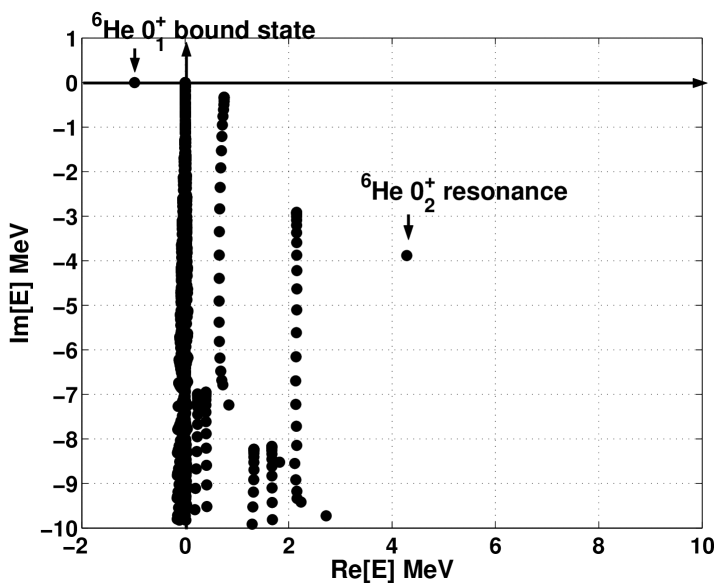
Figure 4: Plot of $0^{+}_{1}$ bound- and $0^{+}_{2}$ resonant state in ⁶He for a model space consisting of the $p_{3/2}$ and $p_{1/2}$ single-particle orbits. The bound and resonant states are well located. The remaining points represent the non-resonant continuum.

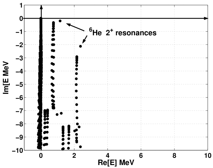
Figure 5: Plot of $2^{+}$ resonances in ⁶He for a model space consisting of the $p_{3/2}$ and $p_{1/2}$ single-particle orbits. Both resonant states are well located. The remaining points represent the non-resonant continuum.

The stability of the $0^{+}$ and $2^{+}$ results as function of the number of mesh points is demonstrated in Tables 2 and 3. Limiting first the attention to a model space consisting only of the $p_{3/2}$ orbit, we note that with $N_{R}=12$ integration points along the rotated path $C_{R}$ and $N_{T}=12$ points along the translated line $C_{T}$, convergence is satisfactory, even with a total of $300$ two-particle states.

Table 2: Convergence of the $0^{+}_{1}$ bound state energy in ⁶He in terms of the number integration points $N_{R}$ and $N_{T}$ along the rotated $C_{R}$ and the translated part $C_{T}$ of the contour, respectively. The number $N_{2p}$ gives the dimension of the two-particle anti-symmetrized basis. Here only $p_{3/2}$ single-particle orbits are included. Energies are given in units of MeV.

$N_{R}$	$N_{T}$	$N_{2p}$	Re[E]	Im[E]
12	12	300	-0.980067	-0.000759
20	20	820	-0.979508	0.000000
25	25	1275	-0.979509	0.000000

Table 3: Convergence of the $2^{+}_{1}$ resonant state energy in ⁶He as function of the number of integration points $N_{R}$ and $N_{T}$ along the rotated $C_{R}$ and the translated part $C_{T}$ of the contour, respectively. The number $N_{2p}$ gives the dimension of the two-particle anti-symmetrized basis. Here only $p_{3/2}$ single-particle orbits are included, and energies are given in units of MeV.

$N_{R}$	$N_{T}$	$N_{2p}$	Re[E]	Im[E]
12	12	300	1.215956	-0.267521
20	20	820	1.216495	-0.267745
25	25	1275	1.216496	-0.267745

Tables 4, 5 and 6 repeat the above convergence analysis, but now employing a model space consisting of the $p_{3/2}$ and $p_{1/2}$ single-particle orbits, and including also the results for the lowest-lying ⁶He state with quantum numbers $J^{\pi}=1^{+}$. Increasing the model space brings several new features. We note in Table 4 that the first excited $0^{+}_{2}$ state is a resonance. However, the stability of the results as functions of the number of mesh points is comparable to that seen in Tables 2 and 3. With approximately $12$ mesh points we obtain results close to the converged ones.

Table 4: Convergence of $0^{+}_{1}$ bound and the $0^{+}_{2}$ resonant state energy in ⁶He as function of the number of integration points $N_{R}$ and $N_{T}$ along the rotated $C_{R}$ and the translated part $C_{T}$ of the contour, respectively. The number $N_{2p}$ gives the dimension of the two-particle anti-symmetrized basis. Here the $p_{3/2}$ and $p_{1/2}$ single-particle orbits are included. Energies in units of MeV.

			$J^{\pi}=0^{+}_{1}$		$J^{\pi}=0^{+}_{2}$
$N_{R}$	$N_{T}$	$N_{2p}$	Re[E]	Im[E]	Re[E]	Im[E]
12	12	600	-0.980111	-0.000497	4.289194	-3.882119
20	20	1640	-0.979148	-0.000000	4.286186	-3.882878
25	25	2550	-0.979148	0.000000	4.286181	-3.882876

Similar conclusions apply to the $1^{+}_{1}$ resonance and the two lowest-lying $2^{+}$ resonant states, see Tables 5 and 6 for more details.

Table 5: Convergence of the $1^{+}_{1}$ resonance as function of the number of integration points $N_{R}$ and $N_{T}$ along the rotated $C_{R}$ and the translated part $C_{T}$ of the contour, respectively. The number $N_{2p}$ gives the dimension of the two-particle anti-symmetrized basis. Here the $p_{3/2}$ and $p_{1/2}$ single-particle orbits are included. Energies in units of MeV.

			$J^{\pi}=1^{+}$
$N_{R}$	$N_{T}$	$N_{2p}$	Re[E]	Im[E]
12	12	1128	1.945539	-2.920286
20	20	3160	1.940263	-2.930619
25	25	4950	1.940266	-2.930608

Table 6: Convergence of the $2^{+}_{1}$ and $2^{+}_{2}$ resonance energy in ⁶He as function of the number of integration points $N_{R}$ and $N_{T}$ along the rotated $C_{R}$ and the translated part $C_{T}$ of the contour, respectively. The number $N_{2p}$ gives the dimension of the two-particle anti-symmetrized basis. Here the $p_{3/2}$ and $p_{1/2}$ single-particle orbits are included. Energies in units of MeV.

			$J^{\pi}=2^{+}_{1}$		$J^{\pi}=2^{+}_{2}$
$N_{R}$	$N_{T}$	$N_{2p}$	Re[E]	Im[E]	Re[E]	Im[E]
12	12	876	1.149842	-0.203052	2.372295	-2.122474
20	20	2420	1.150527	-0.203060	2.372818	-2.123253
25	25	3775	1.150527	-0.203060	2.372817	-2.123254

We note that the experimental value for the width of the first excited $J^{\pi}=2^{+}_{1}$ is $\Gamma\approx 113$ KeV and the energy is $Re[E]_{2^{+}_{1}}=1797$ KeV. Our simplified nucleon-nucleon interaction gives a qualitative reproduction of the data. In a future work we plan to include a realistic nucleon-nucleon interaction for studies of such systems.

We end this subsection by analyzing the squared amplitude of the single-particle configurations ${|RR\rangle,|RC\rangle,|CC\rangle}$ of the $0^{+},1^{+}$ and $2^{+}$ bound- and resonant wave functions. The results are shown in Tables 7,8, 9, 10 and 11. The reason for doing this analysis is due to the fact that our single-particle basis consists of resonant and continuum single-particle orbits. By performing such an analysis we can disentangle the contribution from for example the non-resonant continuum. In these tables, $|RR\rangle$ stands for both single-particle orbits being a resonant single-particle orbit, $|RC\rangle$ means that one single-particle orbit is a resonant single-particle orbit and the other a non-resonant continuum single-particle orbit, while for $|CC\rangle$ both single-particle orbits are from the non-resonant single-particle continuum. All the results show that the configurations where both single-particles are resonant orbits, have the largest amplitude in the two-body wave function. It is also seen, that the configurations where both particles are in complex continuum states have a small effect on the formation of two-particle resonances in ⁶He. This is a useful result which we will exploit below when we define effective interactions for smaller spaces.

Table 7: Expansion coefficients of the $0^{+}_{1}$ bound state in ${}^{6}\mathrm{He}$. The $p_{3/2}$ and $p_{1/2}$ single-particle orbits define the model space. See text for further discussions.

	$\left({p}_{3/2}^{2}\right)$		$\left({p}_{1/2}^{2}\right)$
	Re[$\mathrm{C}^{2}$]	Im[$\mathrm{C}^{2}$]	Re[$\mathrm{C}^{2}$]	Im[$\mathrm{C}^{2}$]
$|RR\rangle$	1.10488	-0.83161	0.22620	-0.16120
$|RC\rangle$	-0.06036	0.88137	-0.19842	0.22423
$|CC\rangle$	-0.09716	-0.04974	0.02486	-0.06305

Table 8: Expansion coefficients of the $0^{+}_{2}$ resonance in ${}^{6}\mathrm{He}$. The $p_{3/2}$ and $p_{1/2}$ single-particle orbits define the model space. See text for further discussions.

	$\left({p}_{3/2}^{2}\right)$		$\left({p}_{1/2}^{2}\right)$
	Re[$\mathrm{C}^{2}$]	Im[$\mathrm{C}^{2}$]	Re[$\mathrm{C}^{2}$]	Im[$\mathrm{C}^{2}$]
$|RR\rangle$	-0.01136	-0.08003	0.90189	0.33029
$|RC\rangle$	0.04282	-0.03939	0.05966	-0.24478
$|CC\rangle$	0.00617	0.00494	0.00082	0.02896

Table 9: Expansion coefficients of the $1^{+}$ resonance in ${}^{6}\mathrm{He}$. The $p_{3/2}$ and $p_{1/2}$ single-particle orbits define the model space. See text for further discussions.

	$\left(p_{1/2}{p}_{3/2}\right)$		$\left({p}_{1/2}^{2}\right)$		$\left({p}_{3/2}^{2}\right)$
	Re[$\mathrm{C}^{2}$]	Im[$\mathrm{C}^{2}$]	Re[$\mathrm{C}^{2}$]	Im[$\mathrm{C}^{2}$]	Re[$\mathrm{C}^{2}$]	Im[$\mathrm{C}^{2}$]
$|RR\rangle$	0.71068	-0.03739
$|RC\rangle$	0.00381	-0.06948	0.00016	0.00003	0.02224	0.01171
$|CR\rangle$	0.20647	0.05208	0.00037	0.00071	0.07067	0.03807
$|CC\rangle$	-0.00984	-0.00149	-0.00031	-0.00009	-0.00424	0.00585

Table 10: Expansion coefficients of the $2^{+}_{1}$ resonance in ${}^{6}\mathrm{He}$. The $p_{3/2}$ and $p_{1/2}$ single-particle orbits define the model space. See text for further discussions.

	$\left(p_{1/2}{p}_{3/2}\right)$		$\left({p}_{3/2}^{2}\right)$
	Re[$\mathrm{C}^{2}$]	Im[$\mathrm{C}^{2}$]	Re[$\mathrm{C}^{2}$]	Im[$\mathrm{C}^{2}$]
$|RR\rangle$	0.11394	-0.00494	0.96962	0.05539
$|RC\rangle$	-0.00474	0.02531	-0.00178	-0.00018
$|CR\rangle$	-0.02776	-0.03796	-0.05069	-0.02708
$|CC\rangle$	0.00229	-0.00772	-0.00089	-0.00282

Table 11: Expansion coefficients of the $2^{+}_{2}$ resonance in ${}^{6}\mathrm{He}$. The $p_{3/2}$ and $p_{1/2}$ single-particle orbits define the model space. See text for further discussions.

	$\left({p}_{1/2}p_{3/2}\right)$		$\left({p}_{3/2}^{2}\right)$
	Re[$\mathrm{C}^{2}$]	Im[$\mathrm{C}^{2}$]	Re[$\mathrm{C}^{2}$]	Im[$\mathrm{C}^{2}$]
$|RR\rangle$	0.88847	-0.03742	0.08911	-0.03742
$|RC\rangle$	-0.04888	0.05674	-0.00104	-0.00055
$|CR\rangle$	0.06058	-0.03336	-0.00072	-0.02469
$|CC\rangle$	0.01131	-0.00447	0.00115	-0.00220

II.4 Three-Particle Resonances in ⁷He

Finally we consider the unbound nucleus ⁷He, whose ground state ($J^{\pi}={3/2}^{-}$) is located $\approx 0.5$ MeV above the ⁶He ground state, with a measured width $\Gamma\approx 160$ keV. Other continuum structures, with tentative spin assignments $J^{\pi}=1/2^{-}$, and $J^{\pi}=5/2^{-}$, have been observed, see for example Ref. jonson for an extensive review of the experimental situation. In this subsection we limit the attention to a model defined by the $p_{3/2}$ single-particle orbits only. Thus our single-particle basis from ⁵He implies that only a $J^{\pi}={3/2}^{-}$ resonance may be formed. The reason we do not include the $p_{1/2}$ single-particle orbits is that we aim at a diagonalization in the full space, taking into account all complex continuum couplings. This model calculation will serve as a later reference. In the case of $24$ mesh points in momentum space for the $p_{3/2}$ single-particle quantum numbers $lj$, the total dimension $d$ of the ($J^{\pi}={3/2}^{-}$) three-particle problem is $d=9224$, if, in addition, we were to include $24$ single-particle momenta for the $p_{1/2}$ single-particle quantum numbers $lj$, we would have roughly $d\sim 40000$ three-body configurations.

In Refs. witek1 and witek2 the dimensionality problem was circumvented by choosing a small number complex continuum states, typically of the order of five, although it was found that a larger number continuum states had to be included to obtain converged results. Our aim in this subsection is to study the full effect of a coupling to the complex continuum, and show that if one is to obtain accurate results, the effect of all particles moving in the continuum on the formation of multi-particle resonances may be important. In addition we include a larger number of continuum states, in order to achieve a satisfactory convergence. As for ⁶He, we construct a three-body wave function using the single-particle wave functions defined in ⁵He. The three-body wave function is expanded in a three-particle anti-symmetric Berggren basis

$$\Psi^{JM}_{\alpha}(1,2,3)=\sum_{a\leq b\leq c}C^{JM}_{(a,b)c}{\Phi}^{JM}_{(a,b)c}(1,2,3),$$

where the completeness relation reads

$$1=\sum_{a\leq b\leq c}|{\Phi}^{JM}_{(a,b)c}(1,2,3)\rangle\langle\tilde{\Phi}^{JM}_{(a,b)c}(1,2,3)|,$$

with

$$1=\sum_{a\leq b\leq c}(C^{JM}_{(a,b)c)})^{2}.$$

The two-body nucleon-nucleon interaction is the same as that used for ⁶He. Fig. 6 gives the energy spectrum after a full diagonalization of the three-particle shell-model equation. It is seen that the choice of contour in calculating the single-particle spectrum is again optimal if we wish to consider the fact that all physical interesting states are well separated from the dense distribution of complex scattering states. The $J^{\pi}=3/2^{-}$ resonance appears at the energy $E_{3/2^{-}}=-(0.12+0.12i)$ MeV.

The plotted energy spectrum shows that the $0^{+}$ and $2^{+}$ states in ⁶He, and the ${3/2}^{-}$ state in ⁵He, form complex thresholds in the energy spectrum of the $J^{\pi}=3/2^{-}$ spectrum in ⁷He, see Tables. 1, 2 and 3. The physical interpretation of these three-particle states is, in the case of the ⁶He thresholds, that two of the neutrons form either the $0^{+}$ ground state or the $2^{+}$ resonant state, while the third neutron is moving in a complex continuum state. A diagonalization within the reduced space, where at most two particles move in continuum states gives the resonance energy $-(0.14+0.16i)$ MeV, which shows that the effect coming from all particles moving in the continuum is not negligible, but small.

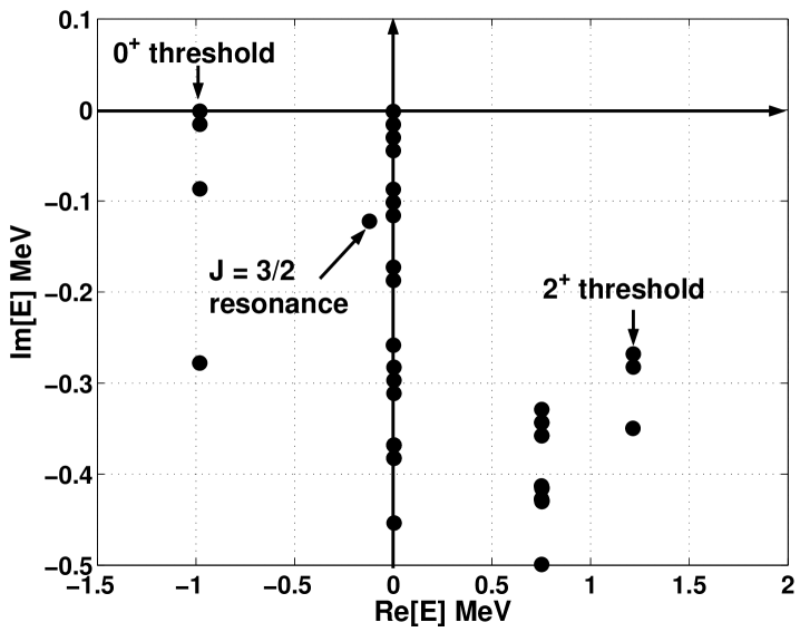
Figure 6: Plot of the ${3/2}^{-}$ complex energy spectrum of ⁷He for a model space consisting of $p_{3/2}$ single-particle orbits only. The $J^{\pi}={3/2}^{-}$ resonance is located at $E_{3/2^{-}}=-(0.120731+0.122211i)$ MeV.

Table 12 gives the squared amplitudes of the various single-particle configurations in the ⁷He ground state, $\{|RRR\rangle,|RRC\rangle,|RCC\rangle,|CCC\rangle\}$ , where $R$ again labels a single-particle resonance and $C$ a complex single-particle continuum orbit. It is seen that the most important configuration, as in the case of ⁶He, is the one where all single-particles are in the $p_{3/2}$ single-particle resonant orbit. The effect of configurations where all particles are in continuum states is small, which suggest that the coupling to configurations $|CCC\rangle$ may be taken into account perturbatively. This a feature we will exploit in Secs. III and IV.

In Fig. 6 we note that the $J^{\pi}=3/2^{-}$ ground state in ⁷He appears at energy of approximately $0.86$ MeV above the ground state in ⁶He, while the experimental value is at approximately $0.5$ MeV. This discrepancy with experiment can be understood in terms of the configuration $|RRR\rangle$, and the choice of interaction. Focusing on the first aspect and using coefficients of fractional parentage, we can rewrite the $|RRR\rangle$ configuration as

$$|(p_{3/2})^{3};\>J^{\pi}=3/2^{-}\rangle={1\over 6}|(p_{3/2})^{2}_{0}\>p_{3/2};\>J^{\pi}=3/2^{-}\rangle-\sqrt{5\over 6}|(p_{3/2})^{2}_{2}\>p_{3/2};\>J^{\pi}=3/2^{-}\rangle.$$

From the geometry one may conclude that the ground state of ⁷He bears much more resemblance with the $2^{+}_{1}$ resonance than with the $0^{+}_{1}$ ground state of ⁶He. In our calculations the $2^{+}_{1}$ resonance comes at an energy $\approx(1.2-0.26i)$ MeV, which is roughly $2.2$ MeV above the $0^{+}_{1}$ ground state of ⁶He, to be contrasted with the experimental value of $\approx 1.8$ MeV, see Fig. 6. This suggests that if we were to increase the attractive strength of the $J^{\pi}=2^{+}$ interaction in ⁶He and get a better agreement with the experimental value, the $J^{\pi}=3/2^{-}$ resonant ground state of ⁷He would get closer to the experimental results.

Table 12: Expansion coefficients of the $J^{\pi}={3/2}^{-}$ ground state in ${}^{7}\mathrm{He}$. Here only $p_{3/2}$ single-particle orbits are included.

$|{p}_{3/2}^{3}\rangle$
	Re[$\mathrm{C}^{2}$]	Im[$\mathrm{C}^{2}$]
$|RRR\rangle$	1.295549	-0.986836
$|RRC\rangle$	-0.184544	1.099729
$|RCC\rangle$	-0.115738	-0.110375
$|CCC\rangle$	0.004733	-0.002518

III Effective Interactions for the Gamow Shell Model

III.1 The Lee-Suzuki Similarity Transformation for Complex Interactions

The previous section served to introduce and motivate the application of complex scaling in studies of weakly bound nuclear systems. However, employing such a momentum space basis soon exceeds feasible dimensionalities in shell-model studies. To circumvent this problem and to be able to define effective interactions of practical use in shell-model calculations, we introduce effective two-body interactions based on similarity transformation methods. These interactions are in turn employed in Gamow shell-model calculations. We base our approach on the extensive works of Suzuki, Okamoto, Lee and collaborators, see for example Refs. suzuki1 ; suzuki2 ; suzuki3 ; suzuki4 . This similarity transformation method has been widely used in the construction of a effective two- and three-body interactions for use in the No-Core shell-model approach of Barrett, Navratil, Vary and collaborators, see for example Refs. bruce1 ; bruce2 ; bruce3 ; bruce4 and references therein. However, since the similarity transformation method has previously only been considered for real interactions, we need to extend its use to Gamow shell-model calculations, implying a generalization to complex interactions. To achieve the latter we introduce first the two-body Schrödinger equation

$$(H_{0}+V_{12})|\psi_{n}\rangle=E_{n}|\psi_{n}\rangle,$$ (9)

here $H_{0}$ includes the single-particle part of the Hamiltonian, kinetic energy and an eventual single-particle interaction. The term $V_{12}$ is the residual two-body interaction. We then expand the exact wave function $\psi_{n}$ in the anti-symmetric two-particle basis, generated by the single-particle basis of $H_{0}$, which corresponds to the basis from the ⁵He calculations of Subsec. II.2. Thereafter we choose a suitable single-particle model space $p$ and its complement space $q$. These single-particle spaces define in turn our two- and many-particle model spaces

$${P}=\sum_{\alpha_{P}}|\alpha_{P}\rangle\langle\tilde{\alpha}_{P}|,$$ (10)

and the complement space

$${Q}=\sum_{\alpha_{Q}}|\alpha_{Q}\rangle\langle\tilde{\alpha}_{Q}|,$$ (11)

where $P$ is defined by both single-particle orbits being in the $p-$space, and the complement space $Q$ is given by all two particle states where at least one particle is in the $q$-space. The anti-symmetric two-particle basis follows the Berggren metric

$$\langle\tilde{\alpha^{\prime}}|\alpha\rangle=\langle{\alpha^{\prime}}^{*}|\alpha\rangle=\delta_{\alpha^{\prime},\alpha},$$ (12)

and the projection operators fulfill the relations

$$P^{2}=P,\;\;Q^{2}=Q,\;\;P^{\mathrm{T}}=P,$$ (13)

and

$$Q^{\mathrm{T}}=Q,\;\;P+Q=1,\;\;PQ=0.$$ (14)

We wish to construct an effective two-body interaction within the model space, reproducing in the $P$-space exactly the $N_{P}$ model space eigenvalues of the full Hamiltonian. This can be accomplished by a similarity transformation

$$\tilde{H}=e^{-\omega}He^{\omega},$$ (15)

where $\omega$ is defined by $\omega=Q\omega P$. It follows that $\omega^{2}=\omega^{3}=...=0$ and $e^{\omega}=P+Q+\omega$. The two-body Schrödinger equation can then be rewritten in terms of a $2\times 2$ block structure

$$\left(\begin{array}[]{cc}P\tilde{H}P&P\tilde{H}Q\\ Q\tilde{H}P&Q\tilde{H}Q\end{array}\right)\left(\begin{array}[]{c}P\psi_{n}\\ Q\psi_{n}\end{array}\right)=E_{n}\left(\begin{array}[]{c}P\psi_{n}\\ Q\psi_{n}\end{array}\right).$$ (16)

If $P\tilde{H}P$ is to be the two-particle effective interaction, the decoupling condition $P\tilde{H}Q=0$ must be fulfilled. One may show that the decoupling condition becomes

$$QHP+QHQ\omega-\omega PHP-\omega PHQ\omega=0,$$ (17)

with $\omega$ acting as a transformation from the model space $P$ to its complement $Q$, viz.,

$$\langle\tilde{\alpha}_{Q}|\psi_{n}\rangle=\sum_{\alpha_{P}}\langle\tilde{\alpha}_{Q}|\omega|\alpha_{P}\rangle\langle\tilde{\alpha}_{P}|\psi_{n}\rangle.$$

There is however no unique solution for $\omega$. The effective interaction generated in the model space depends on the $N_{P}$ exact solutions entering Eq. (III.1). This is why the effective interaction generated by the similarity transformation method is often referred to as a state dependent effective interaction. The solution for $\omega$ may be obtained as long as the matrix $\langle\tilde{\alpha}_{P}|\psi_{n}\rangle$ is invertible and non-singular. Based on this we choose those $N_{P}$ exact solutions with the largest overlap with the two-particle model space. With the solution $\omega$, the non-symmetric effective interaction $R$ is given by

$$R=P\tilde{H}P-PH_{0}P=PV_{12}P+PV_{12}Q\omega.$$ (18)

It would be preferable to obtain a complex symmetric effective interaction, in order to take advantage of the anti-symmetrization of the two-particle basis. This may be accomplished by a complex orthogonal transformation

$$V_{\mathrm{eff}}=U^{-1}(H_{0}+V_{12})U-H_{0},$$ (19)

where $U$ is complex orthogonal and defined by

$$U=\exp(-S),\>\>S=\mathrm{arctanh}(\omega-\omega^{T}),$$ (20)

and

$$U^{T}U=UU^{T}=1,\>\>U^{T}=U^{-1}.$$ (21)

Such complex orthogonal transformations preserve the Berggren metric $x^{T}x$ of any vector $x\in\{C^{n}\}$. This feature allows us to define a complex and symmetric effective two-body interaction

$$V_{\mathrm{eff}}=(P+\omega^{\mathrm{T}}\omega)^{1/2}(PHP+PHQ\omega)(P+\omega^{\mathrm{T}}\omega)^{-1/2}-H_{0}.$$ (22)

In determining $V_{\mathrm{eff}}$, one has to find the square root of the matrix $A=(P+\omega^{\mathrm{T}}\omega)$. In the case of $A$ being real and positive definite the method based on eigenvector decomposition gives generally a stable solution. Using the eigenvector decomposition, with $Z$ representing an orthogonal matrix, $D$ being a diagonal matrix composed of the eigenvalues, using $A=ZDZ^{T}$, $Z^{T}Z=ZZ^{T}=1$, $D=(D)^{1/2}(D)^{1/2}$, and

$$A=\left(ZD^{1/2}Z^{T}\right)\left(ZD^{1/2}Z^{T}\right),$$ (23)

we can write the square root of a matrix $A$ as

$$A^{1/2}=ZD^{1/2}Z^{T}.$$ (24)

For a complex matrix $A$ the procedure based on eigenvector decomposition is generally numerically unstable. An approach suitable for complex matrices is based on properties of the matrix sign function. It can be shown that the square root of the matrix is related to the matrix sign function, see Ref. higham for more details. In the case of $A$ being complex and having all eigenvalues in the open right half complex plane, iterations based on the matrix sign function are generally more stable

$$\mathrm{sign}\left(\left[\begin{array}[]{cc}0&A\\ I&0\end{array}\right]\right)=\left[\begin{array}[]{cc}0&A^{1/2}\\ A^{-1/2}&0\end{array}\right].$$

One stable iteration scheme for the matrix sign was derived by Denman and Beavers denman , as a special case of a method for solving the algebraic Riccati equation

$$Y_{0} = A,\>\>Z_{0}=I,$$ (25)

$$Y_{k+1} = {1\over 2}(Y_{k}+Z_{k}^{-1}),$$ (26)

$$Z_{k+1} = {1\over 2}(Z_{k}+Y_{k}^{-1}),\>\>k=0,1,2,...,$$ (27)

and provided $A$ has no non-positive eigenvalues this iteration scheme exhibits a quadratic convergence rate with

$$Y_{k}\rightarrow A^{1/2},\>\>\>Z_{k}\rightarrow A^{-1/2}\>\>\>\mathrm{as}\>\>\>k\rightarrow\infty.$$ (28)

In our calculations, convergence is typically obtained after a few iterations.

III.2 Gamow Shell-Model Studies of ⁷He with the Similarity Transformation Method

Here we apply the Lee-Suzuki similarity transformation method to the Gamow shell-model calculation of the ground state of ⁷He. The first problem is to define an optimal single-particle model space, which subsequently defines the two-particle model space, where the effective interaction is constructed. In Sec. II it was shown that the $J^{\pi}=3/2^{-}$ ground state of ⁷He has the $2^{+}$ resonance in ⁶He as an important two-body configuration, see Eq. (II.4). Based on this result, a viable starting point is to study the single-particle strengths in the $2^{+}$ resonance wave function. To understand the nature of two-particle resonances and how they are formed in a shell-model framework, it is natural to study and analyze the single-particle strengths in the two-particle wave function, and how they are distributed among the single-particle resonances and the various complex continuum orbits, given on a specific contour in the complex $k$-plane. The single-particle density operator is given by

$$\hat{n}_{i}=\sum_{j}^{N}|{\psi}_{i}(j)\rangle\langle\tilde{\psi}_{i}(j)|,\>\>N=\sum_{i}\hat{n}_{i},$$ (29)

where $N$ is the total number of particles, $i=\{l_{i},j_{i}\}$ labels the single-particle quantum numbers and $i$ represents the single-particle orbit. In the case of ⁶He with an inert ⁴He core, $N=2$. Finding the probability, $n_{i}$, that either particle $1$ or particle $2$ is in the single-particle orbit $i=\{l_{i},j_{i}\}$, we calculate the matrix element of $\hat{n}_{i}$ with the two-particle resonance wave function

$$n_{i} = \langle\tilde{\Psi}_{\alpha}^{J}(1,2)|\hat{n}_{i}|{\Psi}_{\alpha}^{J}(1,2)\rangle=\sum_{a\leq b}\sum_{c\leq d}C_{a,b}^{\alpha}C_{c,d}^{\alpha}\left({1\over(1+\delta_{a,b})(1+\delta_{c,d})}\right)^{1/2}\times$$ (30)

$$\{\delta_{d,i}\>\delta_{c,i}\>\delta_{b,d}+(-1)^{j_{c}+j_{i}-J+1}\delta_{a,i}\delta_{d,i}\delta_{b,c}+\delta_{b,i}\delta_{d,i}\delta_{a,c}+(-1)^{j_{a}+j_{i}-J+1}\delta_{b,i}\delta_{c,i}\delta_{a,d}\}.$$

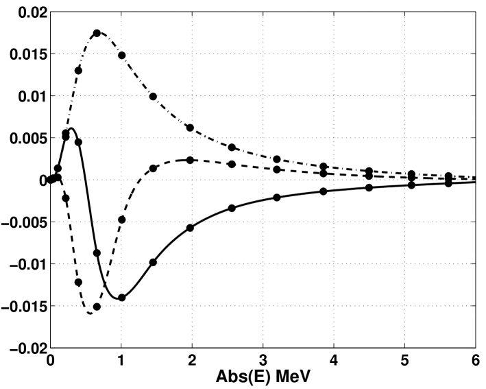
Figure 7: Plot of the $p_{3/2}$ single-particle complex continuum strength $n_{i}$ in the two-particle resonance wave function $2^{+}_{1}$ in ⁶He. The solid line gives the real part, the dotted line the imaginary and the dash-dotted line the absolute value of the strengths. The filled circles give the actual location of the complex continuum states in absolute value of energy.

Fig. 7 gives the real, imaginary and absolute values of the single-particle strengths among the complex continuum orbits, in the $2^{+}$ resonance in ⁶He. The strengths are plotted as a function of the absolute value of the complex continuum energy. Observe that the continuum states near the $2^{+}$ resonance in ⁶He have the largest strengths. This may be understood as an interference effect between the single-particle resonances and the continuum orbits located closest in energy (momentum) to the single-particle resonance. When defining a single-particle model space, we choose the single-particle resonant and complex continuum orbits with the largest absolute value of the single-particle strength. With this recipe we have a consistent way of defining a single-particle model space, which forms the basis for constructing an effective interaction in the two-particle model space.

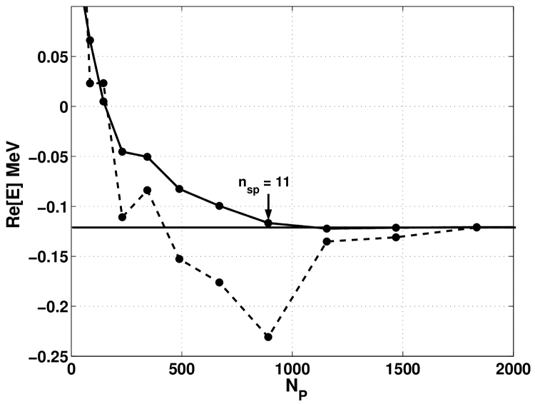
Figure 8: Convergence of the real part of the $J^{\pi}={3/2}^{-}$ resonance in ⁷He for a space defined by the $p_{3/2}$ single-particle orbits only. The abscissa represents the number of three-particle model space configurations $N_{P}$ while $n_{sp}$ represents the total number of single-particle momenta for the $p_{3/2}$ single-particle quantum numbers $lj$. The solid line represents the effective interaction generated by the Lee-Suzuki similarity transformation method, and the dashed line is obtained using the the bare interaction and the same number of three-body configurations. The ${3/2}^{-}$ resonance is located at E $=-(0.120731+0.122211i)$ MeV. The horizontal line is the real energy obtained in the full space of three-body configurations.

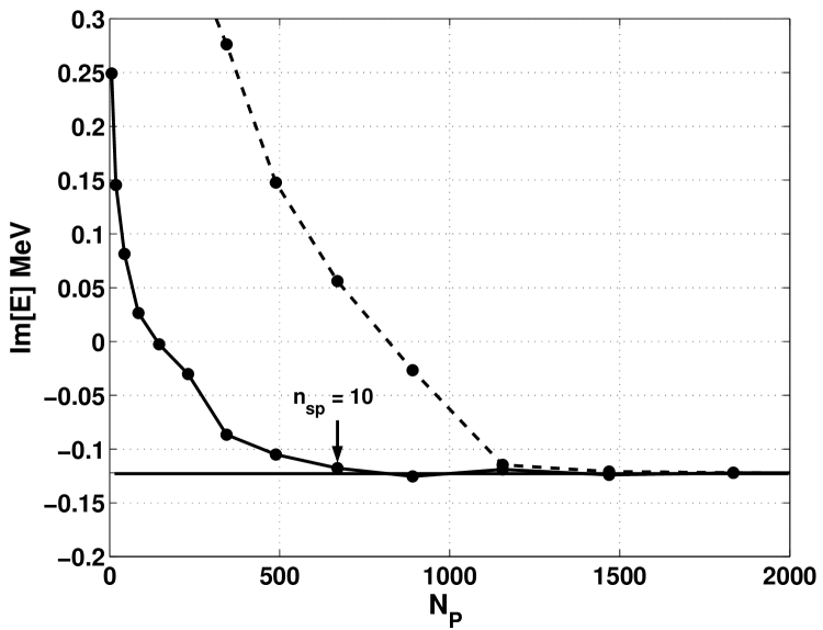
Figure 9: Convergence of imaginary part of $J^{\pi}={3/2}^{-}$ resonance in ⁷He number of three-particle model space configurations$N_{P}$ while $n_{sp}$ represents the total number of single-particle momenta for the $p_{3/2}$ single-particle quantum numbers $lj$. The solid line represents the effective interaction generated by the Lee-Suzuki similarity transformation method, and the dashed line is obtained using the the bare interaction and the same number of three-body configurations. The $J^{\pi}={3/2}^{-}$ resonance is located at E $=-(0.120731+0.122211i)$ MeV. The horizontal line is the imaginary energy obtained in the full space of three-body configurations.

In Figs. 8 and 9 we show the convergence of the real and imaginary part of the $J^{\pi}=3/2^{-}$ resonance in ⁷He, as function of an increasing single-particle model space. For comparison we plot the results for a diagonalization within the model space using the “bare” interaction. It is seen that results with the effective interaction constructed with the similarity transformation method converges much faster than results obtained with the “bare” interaction. We see that a satisfactory convergence is obtained with $10-11$ single-particle Berggren states in the single-particle model space $p$ from ⁵He, corresponding to $\approx 700-800$ three-particle states $N_{P}$. Compared with the full dimension of the three-particle problem, $9224$, we have effectively reduced the dimension to about $8\%$ of the full space. This is a considerable benefit which may allow us to extend the Gamow shell model with a complex scaled single-particle basis to heavier systems and realistic effective interactions. However, we can further improve upon this approach by considering perturbative techniques as well. That is the topic of the next Section.

IV The Multi-Reference Perturbation Method

The Möller-Plesset multi-reference perturbation method has recently been revived in quantum chemistry, see for example Refs. multi1 ; multi2 ; multi3 , with an emphasis on scattering theory and electron decays in many-body systems. Here we only give a brief outline of the method, and refer the reader to Refs. multi1 ; multi2 ; multi3 for further details.

The basic idea of the multi-reference perturbation method is to first diagonalize within a small space (reference space), and then add a perturbation to the reference states by taking into account excitations from the reference space to the complement space.

First we define a suitable $N$-particle reference (model) space $P$ which describes most of the many-body correlations of the system, and hopefully gives a weak coupling with the complement space $Q$. The $N$-body problem may then be written as a block structure

$$\left(\begin{array}[]{cc}H^{PP}&H^{PQ}\\ H^{QP}&H^{QQ}\end{array}\right)\left(\begin{array}[]{c}P\psi_{n}\\ Q\psi_{n}\end{array}\right)=E_{n}\left(\begin{array}[]{c}P\psi_{n}\\ Q\psi_{n}\end{array}\right).$$

Thereafter we divide the full Hamiltonian in two parts

$$\left(\begin{array}[]{cc}H^{PP}&H^{PQ}\\ H^{QP}&H^{QQ}\end{array}\right)=\left(\begin{array}[]{cc}H^{PP}&0\\ 0&D^{QQ}\end{array}\right)+\left(\begin{array}[]{cc}0&H^{PQ}\\ H^{QP}&\tilde{H}^{QQ}\end{array}\right)=H^{0}+H^{1}.$$ (31)

Here $D^{QQ}$ is the diagonal part and $\tilde{H}^{QQ}$ the off-diagonal part of $H^{QQ}$. In this form, we see that $H^{0}$ defines the unperturbed part while $H^{1}$ gives the perturbations to $H^{0}$. In the first step we construct the complex orthogonal matrix $\phi$ which diagonalizes $H^{PP}$. Here the columns of the matrix $\phi$ span the reference space $P$, and is a more convenient basis for perturbation expansions.

Secondly, we perform a standard perturbation expansion in energy, and define $M=\phi^{T}H^{PQ}$ which gives the orthogonal transformation of the coupling block with respect to the reference states $\phi$. Using intermediate normalization, the energy corrections up to third order for a given state $\phi_{i}$ in the reference space, may then be shown to be,

$$E_{i}^{0} = \phi_{i}^{T}H^{PP}\phi_{i},\>\>E_{i}^{1}=0,$$ (32)

$$E_{i}^{2} = \sum_{j=N_{P}+1}^{N}{M_{i,j}^{2}\over E_{i}^{0}-H^{0}_{j,j}},$$ (33)

$$E_{i}^{3} = \sum_{j,k=N_{P}+1}^{N}{M_{i,j}H^{QQ}_{j,k}M_{k,i}^{T}\over(E_{i}^{0}-H^{0}_{j,j})(E_{i}^{0}-H^{0}_{k,k})}\>j\neq k,$$ (34)

here $M_{i,j}$ is the dot product of the vector $\phi_{i}^{T}$ with column $j$ of the coupling block $H^{PQ}$. Observe that there is no first order correction in the energy, meaning that it has been accounted for by the reference states and energies.

In the application of the multi-reference perturbation method to the calculation of multi-particle resonances in Gamow shell-model calculations, we have to define a multi-particle model space which describes most of the many-body correlations. Based on our knowledge from the two-particle system, we assume a good choice for the complement space to consist of configurations where all particles move in complex continuum states. One would expect that the most important configurations of the multi-particle resonance, are configurations which include single-particle resonances. In our calculation of ⁷He, the three-particle model space is chosen by studying the squared amplitudes of the three-particle configurations given in Table 12. There we see that the amplitudes of configurations where all particles move in continuum states are small. In Refs. witek1 and witek2 , where the Helium isotopes ^6-9He were studied within the Gamow shell-model formulation, the authors reached similar conclusions. Note also that we use the bare two-body interaction of Eq. (8). This is to be contrasted to the method outlined in the next section where we use the Lee-Suzuki transformation in order to define an effective interaction.

The three-particle model space, and corresponding complement space, used in our calculations is defined by

$$P\equiv\left\{\begin{array}[]{c}|RRR\rangle,|RRC\rangle,|RCC\rangle,\\ \mathrm{Re}(e_{a}+e_{b}+e_{c})<E_{\mathrm{cut}},\\ \mathrm{Im}(e_{a}+e_{b}+e_{c})>-E_{\mathrm{cut}}\end{array}\right\}\>\>\>Q=1-P,$$ (38)

where at most two particles move in continuum states. We have also introduced a rectangular cutoff in the complex energy plane, since we assume that three-particle configurations high in the energy play a minor role on the formation of low-lying resonances. Fig. 10 gives a plot of the unperturbed three-particle spectrum where at most two particles move in complex continuum states, and three different cut-offs in energies and corresponding model spaces are shown.

Figure 10: Three choices of the model space used in the multi-configuration perturbation method. The three-particle model space states are constructed such that at most two particles move in the non-resonant continuum.

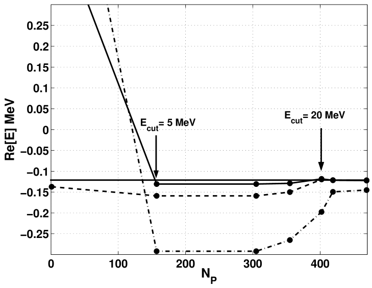
Figure 11: Convergence of the real part of the $J^{\pi}={3/2}^{-}$ resonance in ⁷He, as the dimension of three-particle model space increases with increasing cutoff in energy. The cutoff in energy is increased in steps of $5$ MeV, i.e. $E_{\mathrm{cut}}=0,5,...,30$, and given by the filled circles. The horizontal line is the real part of the $J^{\pi}={3/2}^{-}$ resonance located at E $=-(0.120731+0.122211i)$ MeV. The dashed-dotted line is the zeroth order energy, the dashed line represents the second-order energy and the solid line is the third-order energy.

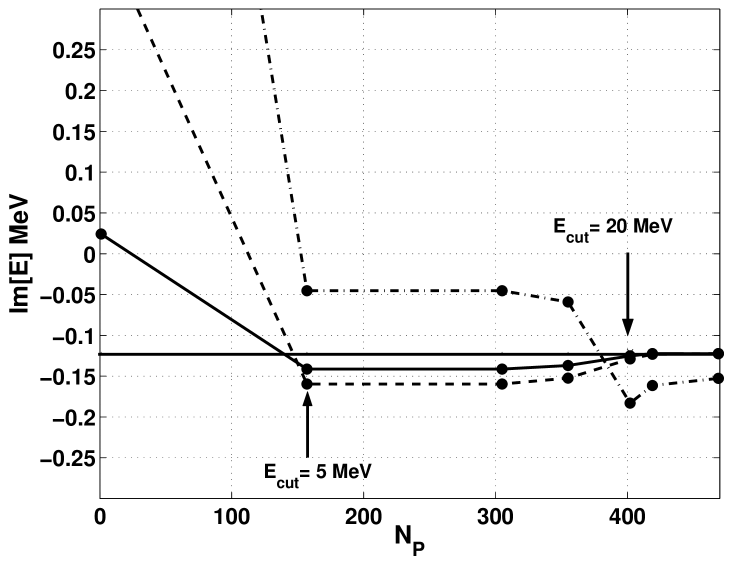
Figure 12: Convergence of the imaginary part of the $J^{\pi}={3/2}^{-}$ resonance in ⁷He, as the number of three-particle model space increases with increasing cutoff in energy. The cutoff in energy is increased in steps of $5$ MeV, i.e. $E_{\mathrm{cut}}=0,5,...,30$, and given by the filled circles. The horizontal line is the the imaginary part of the $J^{\pi}={3/2}^{-}$ resonance located at E $=-(0.120731+0.122211i)$ MeV. The dashed-dotted line is the zeroth order energy, the dashed line represents the second-order energy while the solid line is the third-order energy.

Figs. 11 and  12 show the convergence of the real and imaginary part of the three-particle resonance energy in the multi-reference perturbation method up to third order. The model space used here is given in Eq. 38, and the calculations were done for the increasing cutoffs in energy, $E_{\mathrm{cut}}=0,5,...,30$ MeV. Here the convergence is plotted with respect to the number of three-particle model-space states $N_{P}$ for each energy cutoff. We see that a satisfactory convergence is obtained with $N_{P}\approx 400$, corresponding to the energy cutoff $E_{\mathrm{cut}}=20$ MeV. As expected, we see that excitations of model space configurations located above $E_{\mathrm{cut}}\approx 5$ MeV yield small contributions to the second- and third-order corrections to the resonance energy. Observe that the second- and third-order terms converge at the same number of model space states, which indicates that second-order corrections in energy are seemingly sufficient for our applications. This is also an advantage from a numerical point of view. In second order one has to store only the diagonal part of the block $H^{QQ}$, while in third order the complete block $H^{QQ}$ has be stored, which may be extremely large in many cases. The zeroth order energy, which corresponds to diagonalization within $P$, does not saturate at the exact resonance energy with increasing $N_{P}$, which again shows that possible couplings with the $Q-$ space have to be accounted for, if one aims at accurate calculations.

Summing up these results, we see that we obtain stable results with approximately $N_{P}\approx 400$ three-body configurations within the multi-reference perturbation method, while the similarity transformation method of Sec. III gives stable results for $N_{P}\approx 800$ three-body configurations for the same problem. The question now is whether we can marry these two approaches in our quest for smaller Gamow shell-model spaces. This is the topic of the next section.

V Effective Interaction Scheme for the Gamow Shell Model

In the previous sections it was shown that the Lee-Suzuki similarity transformation and the multi-reference perturbation method may be used in the Gamow shell model in order to account for the most important correlations of for example a multi-particle resonance. Although the dimensionality of the problem derived either from the similarity transformation method or the multi-reference perturbation method was small compared to the full problem, the dimensionality may still be a severe problem when dealing with more than three particles in a big valence space.

The drawback of the multi-reference perturbation method is that one has to store extremely large matrices $H^{QQ}$ if one wishes to go beyond second order in perturbation theory. In the similarity transformation method one does not have to deal with $H^{QQ}$, as couplings with the $Q$-space states have been dealt with, in practical calculations at least at the two-body level. Going to systems with larger degrees of freedom, the $P$-space may nevertheless, at the converged level, be too large for our brute force diagonalization approach.

The aim of this section is to propose an effective interaction and perturbation theory scheme for the Gamow shell model. This approach combines the similarity transformation method and the multi-reference perturbation method, so that hopefully multi-particle resonances where several particles move in large valence spaces, may be calculated without a diagonalization in the full space. Our algorithm is as follows

1. Choose an optimal set of $n_{sp}$ single-particle orbits, which in turn define two-body $P_{2p}$ and many-body spaces. In our case these single-particle orbits are defined by selected states in ⁵He.

2. Construct a two-particle effective interaction by the Lee-Suzuki similarity transformation method within the two-particle model space $P_{2p}$. Such diagonalizations can be done for very large spaces, see for example Refs. bruce1 ; bruce2 ; bruce3 ; bruce4 .

3. The next step is to divide the multi-particle model space $P$ in two smaller spaces $P^{\prime}$ and $Q^{\prime}$, where $P=P^{\prime}+Q^{\prime}$ and $N_{P}=N_{P^{\prime}}+N_{Q^{\prime}}$. The choice of $P^{\prime}$ should be dictated by our knowledge of the physical system. As an example, one may consider those single-particle configurations within the $P-$space that play the dominant role in the formation of the multi-particle resonance. The number $N_{P}=N_{P^{\prime}}+N_{Q^{\prime}}$ represents the total number of many-body configurations within the $P-$space.

4. Now that we have divided the $P$-space in two sub-spaces $P^{\prime}$ and $Q^{\prime}$, we use for example the multi-reference perturbation method to account for excitations from the $P^{\prime}-$ space to the $Q^{\prime}-$ space to obtain energy corrections to a specific order. Increase the size of the $P^{\prime}-$space until convergence is obtained. In the case $N_{P^{\prime}}=N_{P}$ and $N_{Q^{\prime}}=N_{P}-N_{P^{\prime}}=0$ the multi-reference perturbation expansion terminates at zeroth order, and corresponds to a full diagonalization within the $P-$space. Another option is to use for example the coupled cluster method as exposed in Refs. cc1 ; cc2 .

5. Start from top again with a larger set of single-particle orbits, and continue until a convergence criterion is reached.

We illustrate these various choices of model spaces in the following two figures. Fig. 14 defines our model space for the Lee-Suzuki similarity transformation at the two-body level. This corresponds to steps one and two in the above algorithm. The set of single-particle orbits defines the last single-particle orbit in the model space $n_{sp}$. Note that we could have chosen a model space defined by a cut in energy, as done by the No-Core collaboration, see for example Refs. bruce1 ; bruce2 ; bruce3 ; bruce4 . These examples serve just to illustrate the algorithm.

Figure 13: Possible definition of the two-body exclusion operator $Q_{2p}=1-P_{2p}$ used to compute the Lee-Suzuki similarity transformation and its effective interaction at the two-body level. The border of the model space is defined by the last single-particle orbit $n_{sp}$.

Figure 14: Possible definition of many-body space $N_{P}$ and reduced space $N_{P}^{\prime}$.

Fig. 14 demonstrates again a possible division of the space into the full model space $N_{P}$ and a smaller space $N_{P^{\prime}}$. Again, this figure serves only the purpose of illustrating the method. In our actual calculations we define the smaller space $N_{P^{\prime}}$ via an energy cut in the real and imaginary eigenvalues and selected many-body configurations.

In summary, defining a set of single-particle orbits in order to construct the two-body and many-body model spaces, we obtain first an effective two-body interaction in the space $P_{2p}$ by performing the Lee-Suzuki suzuki1 ; suzuki2 ; suzuki3 ; suzuki4 transformation. This interaction and the pertinent single-particle orbits are then used to define a large many-body space. It is therefore of interest to see if we can reduce this dimensionality through the definition of smaller spaces and perturbative corrections.

We present here as a test case, the calculation of the $J^{\pi}=3/2^{-}$ three-particle resonance within the perturbation scheme outlined above. $24$ single-particle orbits for the $lj$ configuration $p_{3/2}$ are included, giving a total dimension of $d=9224$ for the $J={3/2}$ three-particle basis.

We define five different model spaces $P$, given by the total number of three-body configurations $N_{P}$. The number of single-particle orbits and three-body states are listed in Table. 13. The single-particle model space, defining $P$, is constructed according to the prescription outlined in section III. The reference space $P^{\prime}$ which defines a $propersubset$ of each model space $P$, is again defined by

$${P^{\prime}}_{i}\equiv\left\{\begin{array}[]{c}|RRR\rangle,|RRC\rangle,|RCC\rangle\\ \mathrm{Re}(e_{a}+e_{b}+e_{c})<E_{\mathrm{cut}}\\ \mathrm{Im}(e_{a}+e_{b}+e_{c})>-E_{\mathrm{cut}}\end{array}\right\}\>\>\subset P_{i}.$$ (42)

Table 13: Five different $P-$spaces defined for increasing number of single-particle model space orbits $n_{sp}$ consisting of the $lj$ configuration $p_{3/2}$. The number $N_{P}$ gives the dimension of the three-particle model space $P$ for $J^{\pi}=3/2^{-}$ with a full dimensionality with $n_{sp}=24$ of $N_{P}=9224$.

$P$	$P_{1}$	$P_{2}$	$P_{3}$	$P_{4}$	$P_{5}$
$n_{sp}$	8	10	12	14	16
$N_{P}$	344	670	1156	1834	2736

The reader should note that for each space $P_{1}$, $P_{2}$ and so forth listed in Table 13, we can compare the results from this perturbative analysis with those from the exact diagonalization done in these spaces. This is shown in Tables 14,15, 16, 17 and 18.

Table 14: Resonance energy to second (E²) and third order (E³) in the multi-reference perturbation expansion, for the model space $P_{1}$ given in Table  13. The subspaces ${P^{\prime}}_{1}$ are defined for different energy cutoffs, increased in steps of $10$ MeV. In the last line we give the exact energy within $P_{1}$. Energies are given in units of MeV.

	$N_{P_{1}}=344$			$N_{{P^{\prime}_{1}}_{\mathrm{max}}}=113$
$N_{{P^{\prime}}_{1}}$	$N_{Q^{\prime}_{1}}$	$E_{\mathrm{cut}}$	Re[E2]	Im[E2]	Re[E3]	Im[E3]
1	343	0	0.066	0.322	0.606	0.088
113	231	10	0.041	-0.075	0.041	-0.076
Exact within $P_{1}$:			0.042	-0.076

Table 15: Resonance energy to second (E²) and third order (E³) in the multi-reference perturbation expansion, for the model space $P_{2}$ given in Table  13. The subspaces ${P^{\prime}}_{2}$ are defined for different energy cutoffs, increased in steps of $10$ MeV. In the last line we give the exact energy within $P_{2}$. Energies are given in units of MeV.

	$N_{P_{2}}=670$			$N_{{P^{\prime}_{2}}_{\mathrm{max}}}=181$
$N_{P^{\prime}_{2}}$	$N_{Q^{\prime}_{2}}$	$E_{\mathrm{cut}}$	Re[E2]	Im[E2]	Re[E3]	Im[E3]
1	669	0	-0.053	0.357	0.562	0.059
157	513	10	-0.078	-0.110	-0.079	-0.110
181	489	20	-0.082	-0.110	-0.083	-0.110
Exact within $P_{2}$:			-0.081	-0.110

Table 16: Resonance energy to second (E²) and third order (E³) in the multi-reference perturbation expansion, for the model space $P_{3}$ given in Table  13. The subspaces ${P^{\prime}}_{3}$ are defined for different energy cutoffs, increased in steps of $10$ MeV. In the last line we give the exact energy within $P_{3}$. Energies are given in units of MeV.

	$N_{P_{3}}=1156$			$N_{{P^{\prime}_{3}}_{\mathrm{max}}}=265$
$N_{P^{\prime}_{3}}$	$N_{Q^{\prime}_{3}}$	$E_{\mathrm{cut}}$	Re[E2]	Im[E2]	Re[E3]	Im[E3]
1	1155	0	-0.099	0.378	0.561	0.050
205	951	10	-0.114	-0.134	-0.114	-0.133
265	891	20	-0.117	-0.130	-0.118	-0.130
Exact within $P_{3}$:			-0.116	-0.130

Table 17: Resonance energy to second (E²) and third order (E³) in the multi-reference perturbation expansion, for the model space $P_{4}$ given in Table  13. The subspaces ${P^{\prime}}_{4}$ are defined for different energy cutoffs, increased in steps of $10$ MeV. In the last line we give the exact energy within $P_{4}$. Energies are given in units of MeV.

	$N_{P_{4}}=1834$			$N_{{P^{\prime}_{4}}_{\mathrm{max}}}=365$
$N_{P^{\prime}_{4}}$	$N_{Q^{\prime}_{4}}$	$E_{\mathrm{cut}}$	Re[E2]	Im[E2]	Re[E3]	Im[E3]
1	1833	0	-0.134	0.397	0.532	0.026
253	1581	10	-0.155	-0.160	-0.130	-0.141
347	1487	20	-0.119	-0.127	-0.120	-0.126
365	1469	30	-0.122	-0.123	-0.123	-0.124
Exact within $P_{4}$:			-0.121	-0.124

Table 18: Resonance energy to second (E²) and third order (E³) in the multi-reference perturbation expansion, for the model space $P_{5}$ given in Table  13. The subspaces ${P^{\prime}}_{5}$ are defined for different energy cutoffs, increased in steps of $10$ MeV. In the last line we give the exact energy within $P_{5}$. Energies are given in units of MeV.

	$N_{P_{5}}=2736$			$N_{{P^{\prime}_{5}}_{\mathrm{max}}}=419$
$N_{P^{\prime}_{5}}$	$N_{Q^{\prime}_{5}}$	$E_{\mathrm{cut}}$	Re[E2]	Im[E2]	Re[E3]	Im[E3]
1	2735	0	-0.137	0.399	0.530	0.024
253	2483	10	-0.159	-0.160	-0.131	-0.141
347	2389	20	-0.120	-0.129	-0.118	-0.125
409	2327	30	-0.122	-0.122	-0.122	-0.122
419	2317	40	-0.122	-0.122	-0.123	-0.122
Exact within $P_{5}$:			-0.121	-0.122

As the number of reference states $N_{P^{\prime}}$ increases with increasing cutoff in energy $E_{\mathrm{cut}}$, one reaches a maximum of reference states $N_{{P^{\prime}}_{\mathrm{max}}}$ within each $P-$space. From the definition of the reference space $P^{\prime}$ in Eq. (42), it will never coincide with the $P-$space as one exhausts the number of configurations $|RRR\rangle,|RRC\rangle,|RCC\rangle$ within $P$, since one by definition never includes the configurations $|CCC\rangle$, i.e. $\{|P^{\prime}\rangle\}\subset\{|P\rangle\}$. The perturbation scheme for a reference space $P^{\prime}$ given by Eq. (42), will therefore only yield convergent results as long as our assumption that the configurations $|CCC\rangle$ play a minor role compared to the reference states. Although the configurations $|CCC\rangle$ turn out to play a minor role for the states we have considered in this work, there is no a priori reason for this to be the case when considering other multi-particle resonances. If no convergence is observed, one should simply choose another reference space $P^{\prime}$, based for example on the single-particle model space, see Figs. 14 and  14.

Figs. 15 and 16 gives plots of the real and imaginary part of the resonance energy to third order in the multi-reference perturbation expansion for the different model spaces considered above. From the plot one concludes that convergence is obtained for a small number of reference states $N_{P^{\prime}}\sim 350-400$.

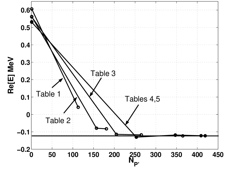
Figure 15: Convergence of the real part of the $J^{\pi}=3/2^{-}$ resonance energy in ⁷He within the perturbative scheme outlined in the text, for the different model spaces $P$ given in Table 13. The open circles along the different solid lines gives the calculations within each $P_{i}$. $N_{P^{\prime}}$ gives the number of reference states in $P^{\prime}$, which is a subspace of $P$. The horizontal line is the the real part of the $J^{\pi}={3/2}^{-}$ resonance located at E $=-(0.120731+0.122211i)$ MeV.

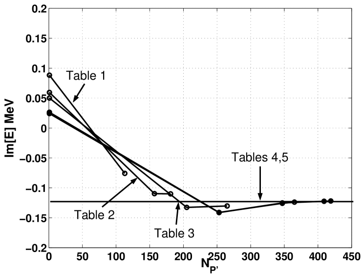
Figure 16: Convergence of the imaginary part of the $J^{\pi}=3/2^{-}$ resonance energy in ⁷He within the perturbative scheme outlined in the text, for the different model spaces $P$ given in Table 13. The open circles along the different solid lines gives the calculations within each $P_{i}$. $N_{P^{\prime}}$ gives the number of reference states in $P^{\prime}$, which is a subspace of $P$. The horizontal line is the the imaginary part of the $J^{\pi}={3/2}^{-}$ resonance located at E $=-(0.120731+0.122211i)$ MeV.

In the approach considered above, the dimension of the $Q^{\prime}-$space is considerably smaller than the dimension of the complement space $Q=1-P$, which makes it much less time and memory consuming to compute the matrix elements of $H^{Q^{\prime}Q^{\prime}}$. We have seen from the above calculations that a termination of the perturbation expansion at second order compares well with the rate of convergence for the third-order expansion. This makes it numerically feasible to treat systems where several particles move in a large valence space, within perturbative scheme outlined above.

We conclude this work by applying our scheme to the calculation of the three-particle resonances in ⁷He, where $24$ single particle states for each of the $lj$ single-particle states $p_{1/2}$ and $p_{3/2}$ are included. The Hamiltonian for the $J^{\pi}=1/2^{-},3/2^{-}$ and $J^{\pi}=5/2^{-}$ states for ⁷He has dimensions $N_{P}=29648,38896$ and $N_{P}=27072$, respectively. The main component of the resonant wave functions turns out to be the $|RRR\rangle$ configuration, which gives the allowed couplings and corresponding unperturbed energies and wave functions $|\left(p_{3/2}\right)^{3};J^{\pi}={3/2}^{-}_{1}\rangle$ with energy $E_{0}=\left(2.2560-0.9840i\right)$ MeV, $|p_{1/2}\>\left(p_{3/2}\right)^{2}_{0};\>J^{\pi}={1/2}^{-}_{1}\>\rangle$ with energy $E_{0}=\left(3.6581-3.5681i\right)$ MeV, $|p_{1/2}\>\left(p_{3/2}\right)^{2}_{2};\>J^{\pi}={3/2}^{-}_{2},\>{5/2}^{-}_{1}\>\rangle$ with energy $E_{0}=\left(3.6581-3.5681i\right)$ MeV and $|\left(p_{1/2}\right)^{2}_{0}\>p_{3/2};J^{\pi}={3/2}^{-}_{3}\rangle$ and energy $E_{0}=\left(5.0602-6.1522i\right)$. We report here only the converged results for the lowest-lying ⁷He resonances. They are $E({3/2}_{1}^{-})=(0.02-0.08i)$ MeV, $E({1/2}_{1}^{-})=(0.39-3.98i)$ MeV, $E({3/2}_{2}^{-})=(2.43-1.95i)$ MeV, $E({5/2}_{1}^{-})=(2.75-0.89i)$MeV, and $E({3/2}_{3}^{-})=(3.85-3.06i)$ MeV. Using our combination of the Lee-Suzuki similarity transformation and the multi-reference perturbation method, results close to the exact ones where obtained with approximately $N_{P^{\prime}}\sim 1400-2000$ three-particle configurations. This is a considerable reduction compared with the full dimensionalities listed above.

Fig. 17 displays the calculated energy levels for the nuclei ^5-7He within our model. The unperturbed energy levels for ⁶He and ⁷He are also shown, and serve to illustrate how the two- and three-particle resonances develop when the nucleon-nucleon interaction from Eq. (8) is included.

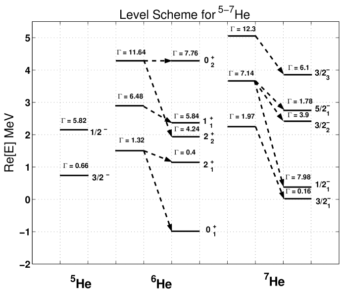
Figure 17: Energy levels for the nuclei ^5,6,7He for model space consisting of the $lj$ single-particle states $p_{1/2}$ and $p_{3/2}$. The unperturbed energy levels for ⁶He and ⁷He are shown to the left in each case.

There are several interesting features which can be seen from Fig. 17. The $0^{+}$- and $2^{+}$-states in ⁶He are formed within our model due to a strong pairing effect between the two neutrons moving in equivalent orbits. When the nucleon-nucleon interaction is included, we observe that the $0^{+}$ and $2^{+}$ unperturbed energies gain an additional attraction. On the other hand, the $1^{+}$ state in ⁶He exhibits weak pairing effects, the main component of the $1^{+}$ wave function is still the configuration $|RR\rangle$, but here the dominant contribution comes from a coupling between the $p_{1/2}$ and $p_{3/2}$ single-particle resonances in ⁵He. Adding the nucleon-nucleon interaction, does not change the unperturbed energy level significantly, see Fig. 17. The calculations done within our crude model of ⁷He, may suggest that this unbound nucleus has an even richer continuum structure than proposed in the recent review of Jonson, see Ref jonson . In Ref. jonson two excited states with tentative spins $J^{\pi}={1/2}^{-}$ and $J^{\pi}={5/2}^{-}$ where reported to exist above the ground state in ⁷He. The level spacings relative to the ⁷He ground state were reported to be $0.57$ MeV and $2.87$ MeV for the $J^{\pi}={1/2}^{-}$ and $J^{\pi}={5/2}^{-}$ states, respectively. The main decay channel of the $J^{\pi}={5/2}^{-}$ resonance at $2.87$ Mev is $\alpha+3n$. From this decay channel, Jonson Ref. jonson concluded that the configuration $|p_{1/2}\>\left(p_{3/2}\right)^{2}_{2};J^{\pi}={5/2}^{-}\rangle$ is the most probable one. In our calculations we find a rich continuum structure in the energy region $\mathrm{Re}[E]\approx 3$ MeV above threshold. From Fig. 17 it is seen that the resonant three-particle states $J^{\pi}={3/2}^{+}_{2},{5/2}^{+}_{2}$ and $J^{\pi}={3/2}^{+}_{3}$ are located rather close in real energy. Although the widths vary from $2-6$ MeV, this observation raises the question of whether these structures may be observed, and which spin assignements and the nature of the experimentally observed structures around $2.87$ MeV in ⁷He are. Further it is seen that the real part of the $J^{\pi}={1/2}^{-}$ resonance changes strongly, and moves towards the threshold when the nucleon-nucleon interaction is included. However, these results must be gauged with the fact that we are using a purely phenomenological nucleon-nucleon interaction model. The inclusion of a realistic interaction is the topic for a future work. The main issue here was to demonstrate how to derive effective interactions for the Gamow shell model, with a considerable reduction in dimensionality.

VI Conclusion and future perspectives.

In this work we have applied the contour deformation method in momentum space, with a single-particle basis in momentum space serving as a starting point for Gamow shell-model calculations. The resonant spectra of the drip-line nuclei ^5-7He have been studied and described using phenomenologically derived nucleon-nucleon interactions. It was illustrated that the choice of contour gives a good convergence for various resonant states, and in addition allows for a clear distinction between all physical states and the remaining complex continuum states. The main purpose of this work was to propose an effective interaction scheme for Gamow shell-model calculations. One of the most severe difficulties regarding Gamow shell-model calculations is the dramatic growth of the shell-model dimension when dealing with several valence particles moving in a large shell-model space. This dimensionality problem is even more severe than the harmonic oscillator representation used in traditional shell-model equation studies, In the Berggren representation a large number of complex-continuum states has to be included as well. The clear distinction of the unperturbed resonances from the dense distribution of complex continuum states, allows for a perturbation treatment, when configuration mixing is taken into account. For perturbation expansions to converge, the unperturbed states have to be well separated from the $Q$-space states, or else the propagators will contain poles which make a perturbative treatment difficult. It has been shown that the Lee-Suzuki similarity transformation combined with the multi-reference perturbation method, reduces the full problem to about $3-4\%$.

Treating the many-particle problem in some perturbation scheme, we need to define a reference (model) space which describes most of the many-body correlations. The method and scheme outlined here, allows for a perturbative treatment of many-body states in which anti-bound states may play an important role, such as in the drip-line nuclei ¹¹Li.

As has been pointed out, the location of multi-particle resonances depends on the effective interaction used between valence nucleons. The next step is to derive a realistic effective interaction for Gamow shell-model calculations, and self-consistent Hartree-Fock single-particle energies for loosely bound nuclei, starting from a realistic nucleon-nucleon force. Using the Berggren representation may give an underlying understanding of many-body resonances from a microscopic point of view. Moreover, in our algorithm of Sec. V we employed the multi-reference perturbation method. Our future plans involve replacing this method by the Coupled Cluster approaches, as discussed in Refs. cc1 ; cc2 .

References

- (1) N. Michel, W. Nazarewicz, and M. Płoszajczak, nucl-th/0407110
- (2) N. Michel, W. Nazarewicz, M. Płoszajczak, and J. Rotureau, nucl-th/0401036
- (3) J. Dobaczewski, N. Michel, W. Nazarewicz, M. Płoszajczak, and M. V. Stoitsov, nucl-th/0401034
- (4) R. J. Liotta, E. Maglione, N. Sandulescu, and T. Vertse, Phys. Lett. B367, 1 (1996).
- (5) R. Id Betan, R. J. Liotta, N. Sandulescu, and T. Vertse, Phys. Rev. C 67, 014322 (2003).
- (6) N. Michel, W. Nazarewicz, M. Płoszajczak, and K. Bennaceur, Phys. Rev. Lett. 89, 042502 (2002).
- (7) N. Michel, W. Nazarewicz, M. Płoszajczak, and J. Okołowicz, Phys. Rev. C 67, 054311 (2003).
- (8) R. Id Betan, R. J. Liotta, N. Sandulescu, and T. Vertse, Phys. Rev. Lett. 89, 042501 (2002).
- (9) R. Id Betan, R. J. Liotta, N. Sandulescu, and T. Vertse, Phys. Lett. B584, 48 (2004).
- (10) A. Volya and V. Zelevinsky, Phys. Rev. C 67, 054322 (2003).
- (11) T. Berggren, Nucl. Phys. A 109, 265 (1968).
- (12) T. Berggren, Nucl. Phys. A 169, 353 (1971).
- (13) T. Berggren, Phys. Lett. B73, 389 (1978).
- (14) T. Berggren, Phys. Lett. B373, 1 (1996).
- (15) P. Lind, Phys. Rev. C 47, 1903 (1993).
- (16) G. Hagen, J. S. Vaagen, and M. Hjorth-Jensen, J. Phys. A: Math. Gen. 37, 8991 (2004).
- (17) B. Jonson, Phys. Rep. 389, 1 (2004).
- (18) N. Moiseyev, Phys. Rep. 302, 211 (1998).
- (19) R. R. Whitehead, A. Watt, B. J. Cole, and I. Morrison, Adv. Nucl. Phys. 9, 123 (1977).
- (20) K. Suzuki and S. Y. Lee, Progr. Theor. Phys. 64, 2091 (1980).
- (21) K. Suzuki, Prog. Theor. Phys. 68, 246 (1982);
- (22) K. Suzuki and R. Okamoto, Prog. Theor. Phys. 92, 1045 (1994); ibid. 93, 905 (1995).
- (23) S. Fujii, E. Epelbaum, H. Kamada, R. Okamoto, K. Suzuki, and W. Göckle, Phys. Rev. C 70, 024003 (2004).
- (24) C. Buth, R. Santra, and L. S. Cederbaum, Phys. Rev. A 69, (2004) 032505.
- (25) F. Chen, E. R. Davidson, and S. Iwata, Int. J. Quantum Chem. 86, (2002) 256.
- (26) R. Santra and L. S. Cederbaum, Phys. Rep. 368, 1 (2002).
- (27) S. Sack, L. C. Biedenharn, and G. Breit, Phys. Rev. 93, 321 (1954).
- (28) P. Navrátil and B. R. Barrett, Phys. Rev. C 57, 562 (1998).
- (29) P. Navrátil, J. P. Vary, and B. R. Barrett, Phys. Rev. Lett. 84, 5728 (2000).
- (30) P. Navrátil, J. P. Vary, and B. R. Barrett, Phys. Rev. C 62 , 054311 (2000).
- (31) P. Navrátil, G. P. Kamuntavicius, and B. R. Barrett, Phys. Rev. C 61 , 044001 (2000).
- (32) N. J. Higham, Num. Algorithms 15, (1997) 227.
- (33) E. D. Denman and A. N. Beavers, Appl. Math. Comput. 2, (1976) 63.
- (34) D. J. Dean and M. Hjorth-Jensen, Phys. Rev. C69, 054320 (2004).
- (35) K. Kowalski, D. J. Dean, M. Hjorth-Jensen, T. Papenbrock, and P. Piecuch, Phys. Rev. Lett. 92, 132501 (2004).