Quantum Monte Carlo Calculations of Light Nuclei

Abstract

Variational Monte Carlo and Green’s function Monte Carlo are powerful tools for calculations of properties of light nuclei using realistic two-nucleon ($N\!N$) and three-nucleon ($N\!N\!N$) potentials. Recently the GFMC method has been extended to multiple states with the same quantum numbers. The combination of the Argonne $v_{18}$ two-nucleon and Illinois-2 three-nucleon potentials gives a good prediction of many energies of nuclei up to ¹²C. A number of other recent results are presented: comparison of binding energies with those obtained by the no-core shell model; the incompatibility of modern nuclear Hamiltonians with a bound tetra-neutron; difficulties in computing RMS radii of very weakly bound nuclei, such as ⁶He; center-of-mass effects on spectroscopic factors; and the possible use of an artificial external well in calculations of neutron-rich isotopes.

1 INTRODUCTION

In the last decade, the Green’s function Monte Carlo (GFMC) method has been developed into a powerful tool for calculations of light nuclei (so far up to $A$ = 12) using realistic two-nucleon ($N\!N$) and three-nucleon ($N\!N\!N$) potentials. GFMC starts with a trial wave function that is obtained via variational Monte Carlo (VMC) and projects out excited state contamination to, in principle, obtain the true ground-state wave function for the given Hamiltonian. In practice the method obtains ground and low-lying excited state energies with an accuracy of 1–2%. A review of the nuclear VMC and GFMC methods up to $A$ = 8 may be found in Ref. [1]; $A$ = 9,10 results are in Ref. [2]. By using the Argonne $v_{18}$ $N\!N$ potential (AV18) and including two- and three-pion exchange $N\!N\!N$ potentials, a series of model Hamiltonians (the Illinois models) were constructed [3] that give a good reproduction of energies for $A$ = 3 to 12. Recently GFMC has been extended to the calculation of multiple excited states with the same quantum numbers [4].

This paper reviews some of these results and compares GFMC energies to No-core Shell Model (NCSM) results [5] for several cases. A recent study showing that an experimental claim of a bound tetraneutron is very unlikely to be valid [6] is also reprised. Finally some on-going work involving spectroscopic factors, neutron-rich oxygen isotopes, and difficulties in GFMC computation of RMS radii is presented.

2 HAMILTONIANS

Our Hamiltonian includes a nonrelativistic one-body kinetic energy, the Argonne $v_{18}$ (AV18) two-nucleon potential [7] and various three-nucleon potentials,

$$H=\sum_{i}(-\frac{\hbar^{2}}{2m}\nabla^{2}_{i})+\sum_{i<j}v_{ij}+\sum_{i<j<k}V_{ijk}\ .$$ (1)

The difference between proton and neutron masses is included in our calculations, but ignored above. The Argonne $v_{18}$ potential is one of a number of accurate $NN$ potential models developed since 1990. It can be written as a sum of electromagnetic and one-pion-exchange terms and a shorter-range phenomenological part. The electromagnetic terms include one- and two-photon-exchange Coulomb interactions, vacuum polarization, Darwin-Foldy, and magnetic moment terms, with appropriate proton and neutron form factors.

The one-pion-exchange part contains the normal Yukawa and tensor functions with a short-range cutoff. This and the remaining phenomenological part of the potential can be written as a sum of eighteen operators, which is where the name $v_{18}$ comes from. The first fourteen are charge-independent, and include spin-spin, tensor, $L\cdot S$, and quadratic-$L$ terms, each with a dependence on isospin. The last four operators break charge independence. The radial forms associated with each operator are determined by fitting $N\!N$ scattering data. The potential was fit directly to the Nijmegen $N\!N$ scattering data base [8], which contains 1787 $pp$ and 2514 $np$ data in the range $0-350$ MeV, with a $\chi^{2}$ per datum of 1.09. It was also fit to the $nn$ scattering length measured in $d(\pi^{-},\gamma)nn$ experiments and the deuteron binding energy.

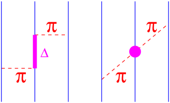
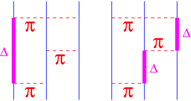
Figure 1: Terms in the Illinois three-nucleon potentials.

The Urbana series of three-nucleon potentials were developed to compute properties of $A=3,4$ nuclei and nuclear matter; the current (ninth) model is designated UIX [9]. These potentials are written as sums of two-pion-exchange with intermediate excitation of an isobar (left panel of Fig. 1) and shorter-range phenomenological terms. The two-pion-exchange term is that of the original Fujita-Miyazawa model [10] and contains both spin (tensor) and isospin dependence. The shorter-range phenomenological term is purely central and repulsive. Our recent work has shown the need for additional binding for $p$-shell nuclei and for further increased binding as $|N-Z|$ increases. This led to the development of the Illinois models [3] which, in addition to the Urbana terms, contain the two-pion $s$-wave scattering term (second panel of Fig. 1) and three-pion exchange ring terms (last two panels of Fig. 1). The latter can involve the excitation of one or two sequential isobars, so that each energy denominator contains only one $\Delta$ mass.

In light nuclei we find that the three-nucleon potential contributes only 2-9% (increasing with $A$) of the total potential energy. However, due to the large cancellation of potential and kinetic energy, this amounts to 15-50% (increasing mostly with $N-Z$) of the binding energy. We expect a similar ratio for the four-body potential, which implies that it contributes only a few percent of the binding energy; such contributions are close to our computational accuracy and would be absorbed in fit of the $N\!N\!N$ potential parameters.

3 QUANTUM MONTE CARLO METHODS

3.1 Variational Monte Carlo

Variational Monte Carlo finds an upper bound, $E_{T}$, to an eigenenergy of $H$ by evaluating the expectation value of $H$ in a trial wave function, $\Psi_{T}$. The parameters in $\Psi_{T}$ are varied to minimize $E_{T}$, and the lowest value is taken as the approximate energy. Over the years, we have developed rather sophisticated $\Psi_{T}$ for light nuclei [11, 12]. A good variational trial function has the form

$$|\Psi_{T}\rangle=\left[1+\sum_{i<j<k}U^{TNI}_{ijk}\right]\left[{\mathcal{S}}\prod_{i<j}(1+U_{ij})\right]|\Psi_{J}\rangle\ .$$ (2)

The $U_{ij}$ and $U^{TNI}_{ijk}$ are non-commuting two- and three-nucleon correlation operators (the most important being the tensor-isospin correlation corresponding to the pion-exchange potential); ${\mathcal{S}}$ indicates a symmetric sum over all possible orderings; and $\Psi_{J}$ is a fully antisymmetric Jastrow wave function which determines the quantum numbers of the state being computed.

The Jastrow wave function, $\Psi_{J}$, for $p$-shell nuclei starts with a sum over independent-particle terms, $\Phi_{A}$, that have 4 nucleons in an $\alpha$-like core and $(A-4)$ nucleons in $p$-shell orbitals. These orbitals are coupled in a $LS[n]$ basis to obtain the desired $JM$ value of a given state, where $n$ specifies the spatial symmetry $[n]$ of the angular momentum coupling of the $p$-shell nucleons. Different possible $LS[n]$ combinations lead to multiple components in the Jastrow wave function. This independent-particle basis is acted on by products of central pair and triplet correlation functions:

$$|\Psi_{J}\rangle = {\mathcal{A}}\left\{\Big{[}\prod_{i<j<k}f^{c}_{ijk}\Big{]}\Big{[}\prod_{i<j\leq 4}f_{ss}(r_{ij})\Big{]}\sum_{LS[n]}\Big{(}\beta_{LS[n]}\Big{[}\prod_{k\leq 4<l\leq A}f^{LS[n]}_{sp}(r_{kl})\Big{]}\right.$$ (3)

$$\times \left.\Big{[}\prod_{4<l<m\leq A}f^{LS[n]}_{pp}(r_{lm})\Big{]}|\Phi_{A}(LS[n]JMTT_{3})_{1234:5\ldots A}\rangle\Big{)}\right\}\ .$$

The operator ${\mathcal{A}}$ indicates an antisymmetric sum over all possible partitions of the $A$ particles into 4 $s$-shell and $(A-4)$ $p$-shell ones. The pair correlation for both particles within the $s$-shell, $f_{ss}$, is similar to that in an $\alpha$-particle. The pair correlations for both particles in the $p$-shell, $f^{LS[n]}_{pp}$, and for mixed pairs, $f^{LS[n]}_{sp}$, are similar to $f_{ss}$ at short distance, but their long-range structure is adjusted to give appropriate clustering behavior, and they may vary with $LS[n]$.

The single-particle wave functions $\Phi_{A}$ are given by:

$$|\Phi_{A}(LS[n]JMTT_{3})_{1234:5\ldots A}\rangle=|\Phi_{4}(0000)_{1234}\Big{[}\prod_{4<l\leq A}\phi^{LS[n]}_{p}(R_{\alpha l})\Big{]}$$ (4)

$$\times\left\{\Big{[}\prod_{4<l\leq A}Y_{1m_{l}}(\Omega_{\alpha l})\Big{]}_{LM_{L}[n]}\Big{[}\prod_{4<l\leq A}\chi_{l}(\frac{1}{2}m_{s})\Big{]}_{SM_{S}}\right\}_{JM}\Big{[}\prod_{4<l\leq A}\nu_{l}(\frac{1}{2}t_{3})\Big{]}_{TT_{3}}\rangle\ .$$

The $\phi^{LS[n]}_{p}(R_{\alpha l})$ are $p$-wave solutions of a particle in an effective $\alpha-N$ potential that has Woods-Saxon and Coulomb parts. They are functions of the distance between the center of mass of the $\alpha$ core and nucleon $l$, and may vary with $LS[n]$. The depth, width, and surface thickness of the single-particle potential are additional variational parameters of the trial function. The overall wave function is translationally invariant, so there is no spurious center of mass motion.

The $\beta_{LS[n]}$ mixing parameters of Eq. (3) are determined by a diagonalization procedure, in which matrix elements

$$E_{T,ij} = \langle\Psi_{T}(\beta_{i})|H|\Psi_{T}(\beta_{j})\rangle\ ,$$ (5)

$$N_{T,ij} = \langle\Psi_{T}(\beta_{i})|\Psi_{T}(\beta_{j})\rangle\ ,$$ (6)

are evaluated using trial functions $\Psi_{T}(\beta_{i})\equiv\Psi_{T}(\beta_{i}=1,\beta_{j\neq i}=0)$. Although the $\Phi_{A}(LS[n]JMTT_{3})$ are orthogonal due to spatial symmetry, the pair and triplet correlations in $\Psi_{T}$ make the different $LS[n]$ components nonorthogonal, so a generalized eigenvalue routine is necessary to carry out the diagonalization.

3.2 Green’s Function Monte Carlo

GFMC projects out the lowest-energy ground state from the VMC $\Psi_{T}$ by using

$$\Psi(\tau) = e^{-({H}-E_{0})\tau}\Psi_{T}~{};$$ (7)

$$\Psi_{0} = \lim_{\tau\rightarrow\infty}\Psi(\tau).$$ (8)

If sufficiently large $\tau$ is reached, the eigenvalue $E_{0}$ is calculated exactly while other expectation values are generally calculated neglecting terms of order $|\Psi_{0}-\Psi_{T}|^{2}$ and higher. In contrast, the error in the variational energy, $E_{T}$, is of order $|\Psi_{0}-\Psi_{T}|^{2}$, and other expectation values calculated with $\Psi_{T}$ have errors of order $|\Psi_{0}-\Psi_{T}|$. Here I present a simplified overview of nuclear GFMC; a rather complete discussion may be found in [11, 12].

Introducing a small time step, $\triangle\tau$, $\tau=n\triangle\tau$, gives (typically $\triangle\tau=0.5$ GeV^-1)

$$\Psi(\tau)=\left[e^{-({H}-E_{0})\triangle\tau}\right]^{n}\Psi_{T}=G^{n}\Psi_{T}\ .$$ (9)

where $G$ is the short-time Green’s function. The $\Psi(\tau)$ is represented by a vector function of $\bf R$, and the Green’s function, $G_{\alpha\beta}({\bf R}^{\prime},{\bf R})$ is a matrix function of $\bf R^{\prime}$ and ${\bf R}$ in spin-isospin space (labeled by the subscripts $\alpha,\beta$), defined as

$$G_{\alpha\beta}({\bf R}^{\prime},{\bf R})=\langle{\bf R}^{\prime},\alpha|e^{-({H}-E_{0})\triangle\tau}|{\bf R},\beta\rangle.$$ (10)

Omitting spin-isospin indices for brevity, $\Psi({\bf R}_{n},\tau)$ is given by

$$\Psi({\bf R}_{n},\tau)=\int G({\bf R}_{n},{\bf R}_{n-1})\cdots G({\bf R}_{1},{\bf R}_{0})\Psi_{T}({\bf R}_{0})d{\bf R}_{n-1}\cdots d{\bf R}_{1}d{\bf R}_{0},$$ (11)

and the integration is done by Monte Carlo. We approximate the short-time propagator as a symmetrized product of exact two-body propagators and include the $V_{ijk}$ to first-order. In recent benchmark calculations [13] of ⁴He using an eight-operator NN potential, the GFMC energy had a statistical error of only 20 keV and agreed with the other best results to this accuracy ($<$ 0.1%).

For more than four nucleons, GFMC calculations suffer significantly from the well-known Fermion sign problem. This results in exponential growth of the statistical errors as one propagates to larger $\tau$, or as $A$ is increased. For $A\geq 8$ the resulting limit on $\tau$ is too small to allow convergence of the energy. In the last few years we have developed and extensively tested a constrained-path algorithm for nuclear GFMC [12] to solve this problem. In this method configurations with small or negative $\Psi(\tau)^{\dagger}\!\cdot\!\Psi_{T}$ are discarded such that the average over all discarded configurations of $\Psi(\tau)^{\dagger}\cdot\Psi_{T}$ is 0. This means that, if $\Psi_{T}$ were the true eigenstate, the discarded configurations would contribute nothing but noise to $\langle H\rangle$. This constrained propagation completely controls the growth of the statistical errors and in most cases produces a result that is statistically the same as unconstrained propagation (the accuracy of the comparison may be limited by the statistical errors in the unconstrained result). However we have demonstrated some cases for which constrained propagation leads to a wrong result, and in fact for which the approximate $\langle H\rangle$ is not even an upper bound to the correct eigenvalue. In all cases the correct result can be obtained by making a few (10 to 20) unconstrained steps before evaluating the energy. Our calculations for $A\geq 5$ are now all made using constrained-path propagation with 10 to 20 unconstrained steps.

The number of spin-isospin components in $\Psi_{T}$ grows rapidly with the number of nucleons. Thus a calculation of a state in ⁸Be involves about 30 times more floating-point operations than one for ⁶Li, and ¹⁰Be requires 50 times more than ⁸Be. Calculations of the sort being described here are currently feasible up to only $A=12$; for $A$=10, these require $\sim$8,000 processor hours on the NERSC IBM SP (Seaborg) running at 390 MFLOPS/processor ($10^{16}$ operations) and $\sim$150,000 processor hours for ¹²C on the Los Alamos qsc computer running at 360 MFLOPS/processor ($2\times 10^{17}$ operations).

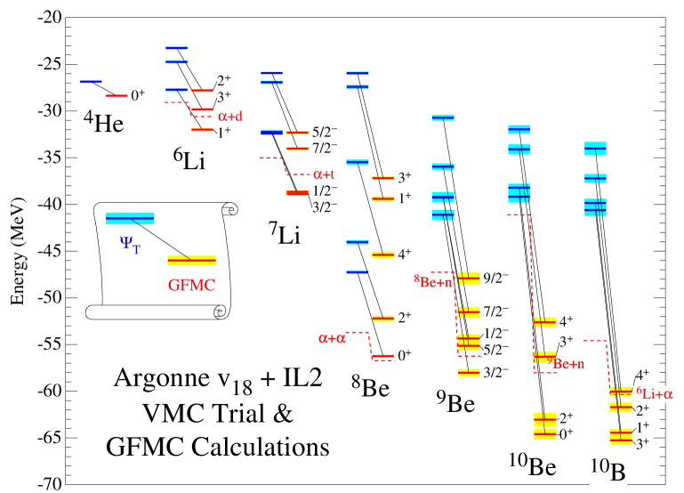
Figure 2: Comparison of $\Psi_{T}$ and GFMC energies for several nuclei

Figure 2 compares the VMC and GFMC energies of several nuclei for the AV18+IL2 Hamiltonian. We see that the variational wave functions for the $s$-shell nuclei are quite accurate–the GFMC improves our best VMC energy of ⁴He by only 1.5 MeV or 5%. (These $\Psi_{T}$ do not contain explicit correlations for the new terms in the Illinois $N\!N\!N$ potential; the corresponding error for the AV18+UIX Hamiltonian is only 2%.) However, the $p$-shell variational wave functions are much less accurate; compared to the GFMC energies, they result in underbindings of 4.3 MeV (13%) for ⁶Li to 25 MeV (38%) for ¹⁰B. In fact the $\Psi_{T}$ fail to give particle-stable energies for any of the $A\geq 6$ nuclei and give maximum binding energies for ⁸Be. On the other hand, the excitation spectra from VMC and GFMC calculations are generally quite similar, except when there is a change in the dominant symmetry.

3.3 GFMC Evaluation of Excited States

It is possible to treat at least a few excited states with the same quantum numbers using VMC and GFMC methods [4]. The VMC calculations have been described above, and essentially involve solving a generalized eigenvalue problem, Eqs. (5) and (6). The same basic method can be applied in GFMC calculations, though the implementation is slightly more involved. In this section, $\Psi_{T,i}$ represents the trial wave function for the $i^{th}$ state of specified $(J^{\pi},T)$ and $\Psi_{i}(\tau)$ is the GFMC wave function propagated from it. By construction $\langle\Psi_{T,i}|\Psi_{T,j}\rangle=0$ for $i\neq j$. We would like to calculate the Hamiltonian and normalization matrix elements as a function of $\tau$:

$$H_{ij}(\tau) = \frac{\langle\Psi_{i}(\tau/2)|\ H\ |\Psi_{j}(\tau/2)\rangle}{|\Psi_{i}(\tau/2)||\Psi_{j}(\tau/2)|},$$ (12)

$$N_{ij}(\tau) = \frac{\langle\Psi_{i}(\tau/2)|\Psi_{j}(\tau/2)\rangle}{|\Psi_{i}(\tau/2)||\Psi_{j}(\tau/2)|},$$ (13)

where $|\Psi_{i}|=|\langle\Psi_{i}|\Psi_{i}\rangle|^{1/2}$. Solving the generalized eigenvalue problem with these Hamiltonian and normalization matrix elements would yield improved upper bounds for the ground and low-lying excited states of the system. In the limit $\tau\rightarrow\infty$ the solutions would be exact.

In GFMC we can compute mixed expectation values such as

$$\tilde{O}_{ij}(\tau)=\frac{\langle\Psi_{i}(\tau)|\ O\ |\Psi_{T,j}\rangle}{\langle\Psi_{i}(\tau)|\Psi_{T,i}\rangle},$$ (14)

where the denominator involves just state $i$. Since the propagator commutes with the Hamiltonian, the desired matrix elements can be computed as:

$$H_{ij}(\tau) = [\tilde{H}_{ij}\tilde{H}_{ji}]^{\mbox{$\textstyle{1\over 2}$}},$$ (15)

$$N_{ij}(\tau) = [\tilde{N}_{ij}\tilde{N}_{ji}]^{\mbox{$\textstyle{1\over 2}$}},$$ (16)

where we use expectation values computed from separately propagated $\Psi_{i}(\tau)$ and $\Psi_{j}(\tau)$. For $i=j$ these equations reduce to the standard GFMC calculation described above.

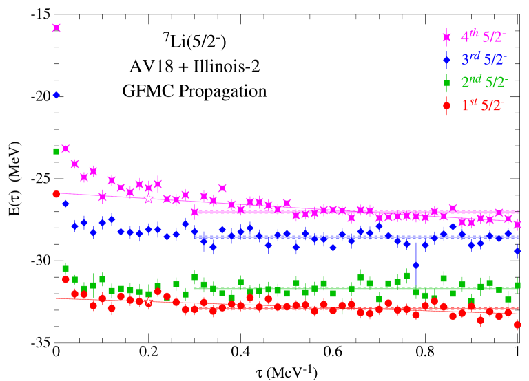
Figure 3: GFMC energies of four $\frac{5}{2}^{-}$ states in ⁷Li versus imaginary time, $\tau$.

As an example, Fig. 3 shows the computation of the energies of four $\mbox{$\textstyle{5\over 2}$}^{-}$ states in ⁷Li. The lowest state has mainly [43] symmetry and can easily decay to the $\alpha$+t channel; it has a large experimental width (918 keV) and its computed energy is slowly decreasing to the energy of the separated clusters. The remaining states are mainly of [421] symmetry and so are principally connected to the ⁶Li+n channel. The second $\mbox{$\textstyle{5\over 2}$}^{-}$ state is experimentally just above the ⁶Li+n threshold and has a small width (80 keV); its computed energy becomes constant with increasing $\tau$. The last two $\mbox{$\textstyle{5\over 2}$}^{-}$ states are not experimentally known, but the very slow decrease with $\tau$ of the energy of the third state suggests that this state may also be narrow. The off-diagonal overlaps $N_{i1}(\tau)$ are small and do not show signs of steadily increasing with increasing $\tau$. The solutions of generalized eigenvalue problems using the $E_{ij}(\tau)$ and $N_{ij}(\tau)$ are not significantly different from the $E_{ii}(\tau)$ shown in the figure. These results show that the (constrained) GFMC propagation largely retains the orthogonality of the starting $\Psi_{T,i}$. Contrary to what might have been expected, the propagation of the higher states does not quickly collapse to the lowest state.

4 ENERGIES OF NUCLEAR STATES

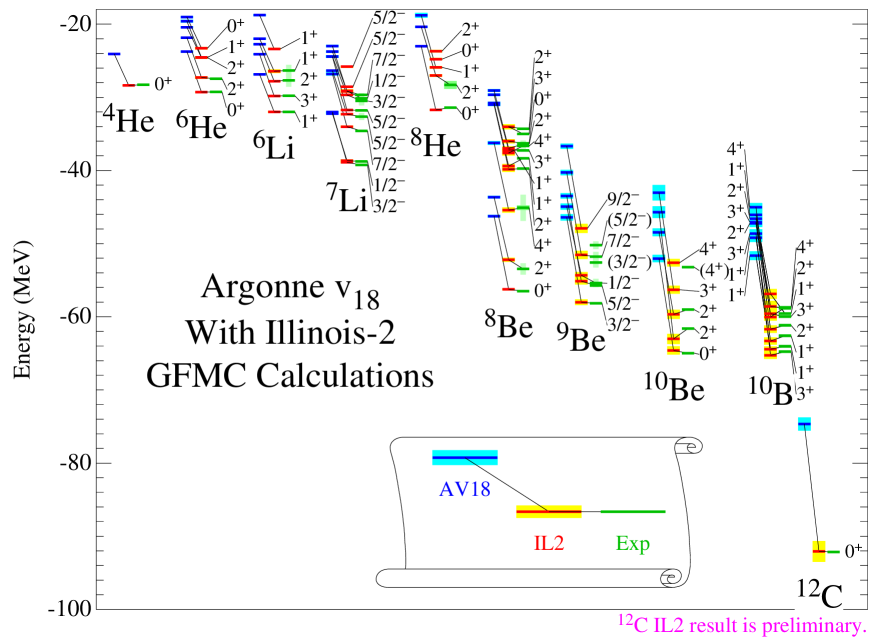
Figure 4: Energies of nuclear states computed with just the AV18 $N\!N$ potential, and with the addition of the IL2 $N\!N\!N$ potential, compared to experiment.

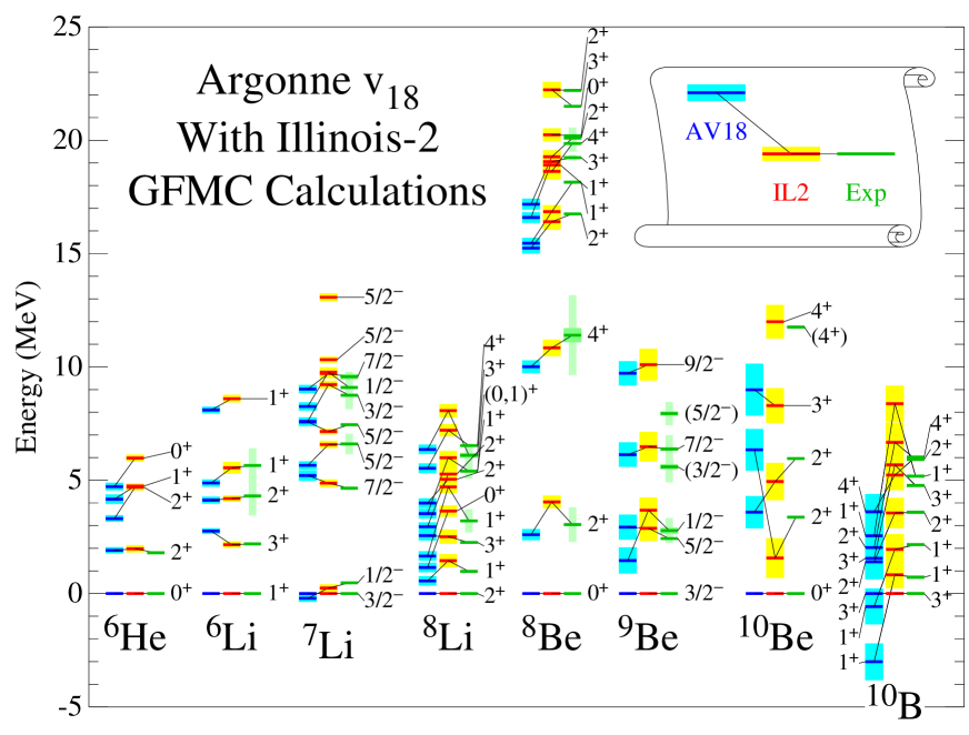
Figure 5: Excitation energies of nuclear states.

Figure 4 compares energies computed with the AV18 (no $V_{ijk}$) and AV18+IL2 Hamiltonians to experimental values. The AV18+IL2 result shown for ¹²C was made using a simplified $\Psi_{T}$ and an approximate treatment of $V_{ijk}$ in the GFMC propagation; for these reasons it is marked preliminary. We see that using just a $N\!N$ potential underbinds ⁴He by 4 MeV; this underbinding increases to 18 MeV for ¹²C. The parameters of the Illinois-2 $N\!N\!N$ potential were adjusted to reproduce the energies of 17 narrow states for $3\leq A\leq 8$ [3]. As can be seen the potential provides an excellent overall reproduction of the energies of many states up to the ground state of ¹²C; the RMS error in reproducing the experimental energies of the 39 states with width $<0.2$ MeV is 0.7 MeV.

Figure 5 shows excitation spectra of nuclei. One again sees a generally good reproduction using AV18+IL2 of the experimental values. The $N\!N\!N$ potential increases the predicted splittings of several spin-orbit partners, such as the $3^{+}$,$2^{+}$,$1^{+}$ triplet in ⁶Li and the first $\mbox{$\textstyle{7\over 2}$}^{-}$ and $\mbox{$\textstyle{5\over 2}$}^{-}$ levels in ⁷Li which significantly improves the agreement with experiment. A variational study of ¹⁵N also showed that a large part of the spin-orbit splitting in that nucleus is a result of the $N\!N\!N$ potential [14]. However the most dramatic effect of the $N\!N\!N$ potential on levels appears in ¹⁰B. The AV18 Hamiltonian results in two $1^{+}$ levels being below the $3^{+}$ state which is the experimental ground state; the AV18+IL2 Hamiltonian gives the correct order. A similar inversion of levels occurs for the $\mbox{$\textstyle{5\over 2}$}^{-}$ and $\mbox{$\textstyle{1\over 2}$}^{-}$ states in ⁹Be. These inversions are also due to increased spin-orbit strength from the $N\!N\!N$ potential; in 1956 Kurath showed that the position of the ¹⁰B(3⁺) state depends sensitively on spin-orbit strength [15]. Another level ordering that is correct only with the $N\!N\!N$ potential is shown in ¹⁰Be. Here, as can be inferred from the experimental $BE(2)$’s to the ground state, the first $2^{+}$ level should have a large negative quadrupole moment and the second should have a positive quadrupole moment. This is the case for the full AV18+IL2 Hamiltonian but without IL2 the energies of these states are reversed.

5 OTHER RESULTS

5.1 Comparison of GFMC and No-core Shell Model Calculations

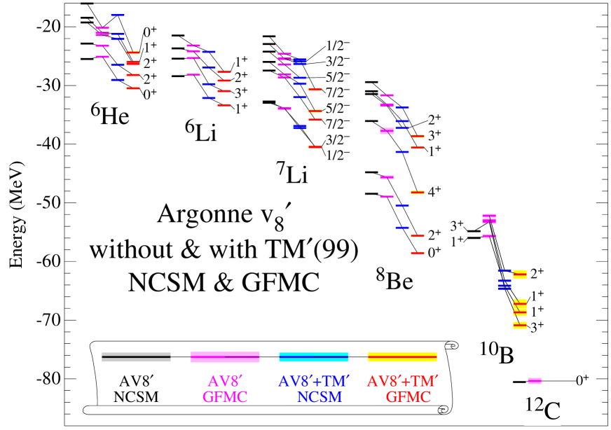
Figure 6: Comparison of NCSM and GFMC energies for the AV8^′ and AV8^′+TM^′ Hamiltonians.

The no-core shell model (NCSM) is an alternative many-body method that uses realistic $N\!N$ and $N\!N\!N$ potentials for light nuclei. It uses an expansion in a large harmonic-oscillator basis for all $A$ nucleons. Effective two- and three-body interactions are constructed from the bare $v_{ij}$; bare $V_{ijk}$ can also be included in the three-body effective interactions. The construction of the effective interactions also gives a unique prescription for constructing effective operators from bare operators. The size of the harmonic-oscillator basis for a specified order of expansion grows rapidly with $A$. At present 16$\hbar\Omega$ can be used for $A=6$ with just two-body effective interactions; this results in well-converged calculations. However only 8$\hbar\Omega$ can be used for $A=12,16$ and two-body effective interactions and these calculations are not fully converged. Calculations with three-body effective interactions are limited to 6$\hbar\Omega$ and are generally not converged. For a complete description of this method see [5] and references therein.

The NCSM is much faster than GFMC but because of these limits on the basis size appears to be less accurate than GFMC, especially when a $N\!N\!N$ potential is being used. This is shown in Fig. 6 in which NCSM and GFMC calculations of several nuclei are compared. The left-hand two bars for each state show, respectively, NCSM and GFMC calculations for the AV8^′ potential [11] with no $N\!N\!N$ potential; there is good agreement between both methods. The right-hand two bars shows results with the TM^′(99) $N\!N\!N$ potential [16] added to AV8^′. In this case the NCSM results are significantly above those from GFMC; that is the NCSM appears to not get the full additional attraction provided by TM^′(99). This is probably because of the limitation to only 6$\hbar\Omega$ when using the three-body effective interaction.

5.2 Can Modern Nuclear Hamiltonians Tolerate a Bound Tetraneutron?

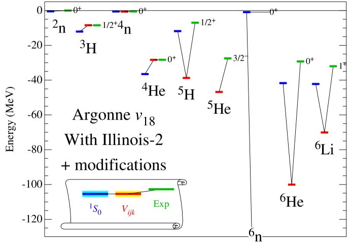
Figure 7: Predictions of Hamiltonians that have been modified to bind a tetraneutron.

An experimental claim of the existence of a bound tetraneutron cluster (⁴n) was made recently [17]. This prompted our study [6] of the theoretical possibility of such a state; the conclusion was that a bound tetraneutron is strongly excluded by modern nuclear Hamiltonians. As a first step, negative-energy ⁴n solutions using the AV18+IL2 model were searched for; GFMC calculations, using propagation to very large imaginary time ($\tau=1.6$ MeV^-1), produced only positive energies that steadily decreased as the RMS radius of the system increased. Adding artificial external wells to the Hamiltonian can, of course, produce negative energies. By varying the well depth, one can extrapolate to zero-well depth. Such calculations suggest that there might be a ⁴n resonance near +2 MeV, but since the GFMC calculation with no external well shows no indication of stabilizing at that energy, the resonance, if it exists at all, must be very broad.

To study the possibility that a minor modification of the AV18+IL2 model could result in binding of ⁴n, a number of modifications to the AV18+IL2 model were made. In each case the modification was adjusted to bind ⁴n with an energy of approximately $-0.5$ MeV; the consequences of this modification for other nuclei were then computed. Figure 7 shows some of these results. In the first such modification, the AV1^′ potential [18] was used in just the ${}^{1}\!S_{0}$ partial wave (and AV18 in the other partial waves); this results in a ⁴n energy of $-0.52$ MeV. However, as is shown by the bars labeled ${}^{1}\!S_{0}$ in the figure, this results in substantial overbinding of ³H, ⁴He and all other nuclei that were computed. In addition it results in a bound dineutron; in fact the ⁴n is not really bound as it can decay into two dineutrons.

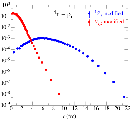
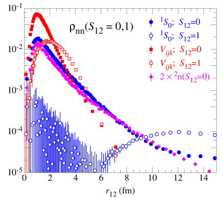
Figure 8: One- and two-body densities of ⁴n bound with either a modified ${}^{1}\!S_{0}$ (circles) or $T=3/2$ $N\!N\!N$ potential (squares). The diamonds show twice the two-body density of ²n. Two-body densities are shown projected into total spin 0 or 1 channels.

Modifications to the $N\!N\!N$ or $N\!N\!N\!N$ potentials, which are experimentally much less constrained than the $N\!N$ potential, could be used to bind ⁴n. A $N\!N\!N$ potential that acts only in $T=\mbox{$\textstyle{3\over 2}$}$ triples would have the same effect on ⁴n as one with no isospin dependence, but would have no effect on ³H and ⁴He because they contain only $T=\mbox{$\textstyle{1\over 2}$}$ triples. Such a potential was added to the AV18+IL2 Hamiltonian, and the coupling constant chosen to produce ⁴n with $\sim-0.5$ MeV energy. It turns out that the coupling must be quite large to produce the minimally bound ⁴n.

This can be understood as follows. If a modified $N\!N$ potential is used to bind ⁴n, the pairs can sequentially come close enough to feel the attraction; this allows the four neutrons to be in a diffuse, large radius, distribution. However a $N\!N\!N$ potential requires three neutrons to simultaneously be relatively close and thus the density of the system must be much higher. Indeed the RMS radii of the ⁴n for the modified $N\!N\!N$ potential is only 1.9 fm while the RMS radius for ${}^{4}n$ produced by the modified $N\!N$ potential is 10 fm. The left panel of Fig. 8 shows the corresponding densities. The right panel compares the pair distributions for the two different ⁴n systems with that of the dineutron made by the modified $N\!N$ potential. The $S=0$ pairs in the ⁴n made by the modified $N\!N$ potential are basically undisturbed ²n pairs, while the modified $N\!N\!N$ potential results in very different ²n pairs.

The small radius of the ⁴n bound by the modified $N\!N\!N$ potential results in a kinetic energy that is an order of magnitude more than for the ⁴n bound by the modified ${}^{1}\!S_{0}$ potential. This large kinetic energy must be overcome by a large $N\!N\!N$ potential energy, and hence a large coupling constant is required.

The very large coupling constant for the extra $N\!N\!N$ term means that it has a large, even catastrophic, effect on any nuclear system in which it can act. This is shown in Fig. 7 by the bars labeled $V_{ijk}$; for example the binding energy of ⁶Li is doubled and that of ⁶He is tripled. As stated above, this potential has no effect on ³H or ⁴He. However the most dramatic result of this potential is that every investigated pure neutron system with $A>4$ is extremely bound and in fact is the most stable “nucleus” of that A; the ⁶n energy is off the scale of the figure at -650 MeV!

A four-nucleon potential that acts in only $T=2$ quadruples was also constructed to weakly bind ⁴; it has even more devastating consequences for nuclei in which it can act than the $N\!N\!N$ potential. Thus an experimental observation of a bound tetraneutron would not be a minor perturbation to our understanding of nuclei; the experimental evidence for such a claim should be very strong before it is taken seriously.

5.3 RMS radii of helium isotopes

Recently a group at Argonne has measured the RMS charge radius of the radioactive nucleus ⁶He ($\beta$-decay halflife 0.8 sec.) with the remarkable accuracy of 0.7% [19]. This prompted us to revisit our already published [3] proton RMS radius for ⁶He. That calculation had been made with our standard propagation to $\tau=0.2$ MeV^-1 and had produced a value in excellent agreement with the new experimental value. We made new calculations to much larger $\tau$ and found that there are very slow fluctuations of the RMS radius with $\tau$. These are shown in Fig. 9 which contains a GFMC propagation to $\tau=7.25$MeV^-1 for ⁶He using the AV18+IL2 Hamiltonian. The upper panel shows the energy on a highly magnified scale; the results show just Monte Carlo statistical fluctuations with no long-term correlations. The standard error of the mean that is extracted from these numbers is thus reliable. However the RMS point proton radius shown in the lower panel has extremely long-range correlations making the error of the mean a useless number. We do not understand the origin of these fluctuations and have been unable to reduce them by using different importance sampling methods in the GFMC propagation. At the moment all we can do is report the average shown in the figure and use the extrema of the fluctuations as an estimate of the error; after folding in the proton and neutron RMS radii, this is reported in Table 1 as a charge radius. As can be seen our computed value is significantly above the experimental value. We have also made a large-$\tau$ calculations of the RMS radii of ⁴He and ⁸He. The ⁴He calculation shows no long-term fluctuations and that of ⁸He shows substantially smaller fluctuations than for ⁶He. These results are also reported in the table.

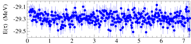
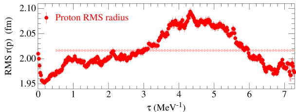
Figure 9: GFMC propagation of ⁶He energy (top panel) and RMS point proton radius (bottom panel).

Table 1: Computed and experimental RMS charge radii (in fm) of helium isotopes

	AV18+IL2	Expt.
4He	1.660(10)	1.673(1)
6He	2.15(7)	2.054(14)
8He	1.98(4)

5.4 Center of Mass Effects on Spectroscopic Factors

Spectroscopic factors are a measure of probability of finding subcluster structure in a nucleus. For the case of a specific $A$-1 nuclear state in an $A$-body nucleus they are defined by computing the quasi-hole wave function for nucleon removal:

$$\chi(r)=\langle[\Psi_{A-1}(J^{\prime})\times N(\ell_{j})]_{{}_{J}}|a(r)|\Psi_{A}(J)\rangle~{}~{}~{}.$$ (17)

The spectroscopic factor is then

$$\mathcal{S}=\int drr^{2}|\chi(r)|^{2}~{}~{}~{}.$$ (18)

It is straightforward to compute $\mathcal{S}$ from shell-model wave functions. Conventional shell model calculations are done in a fixed center (FC) with harmonic oscillator wave functions. Dieperink and de Forest [20] showed how to convert such $\mathcal{S}$ to the desired translationally invariant (TI) ones. For the case of removing a single nucleon from the $p$ shell, their formula becomes

$$\mathcal{S}_{\mathtt{TI}}=\frac{A}{A-1}\mathcal{S}_{\mathtt{FC}}~{}~{}~{}.$$ (19)

This increase of $\mathcal{S}$ arises from the center of mass acquiring a $L=1$ component from the $p$-shell nucleons. This means that the nominally $s$-shell core nucleons have some $p$-wave component and thus contribute to the $p$-wave spectroscopic factors; $s$-wave spectroscopic factors are reduced to conserve the total number of nucleons.

This theorem assumes that the same oscillator parameter is being used for $s$- and $p$-shell nucleons. However, this is not a realistic assumption; if the oscillator parameter is chosen to give a good RMS radius for the $s$-shell core (⁴He) then very small RMS radii will be obtained for the $p$-shell nuclei. An example is shown in Table 2 which shows several calculations of spectroscopic factors for removing a proton from the ground state of ⁷Li. The rows show various cases from an uncorrelated shell model to experimental values. The columns show the point RMS radii of ⁷Li and the spectroscopic factors computed in a fixed center and with translationally-invariant wave functions. For each case the spectroscopic factors to the ground state (0⁺) of ⁶He and the sum of the factors for the 0⁺ and 2⁺ states are shown. The final column shows the ratio of the TI to FC sums.

Table 2: Spectroscopic factors for ⁷Li($\mbox{$\textstyle{3\over 2}$}^{-}$) $\rightarrow$ ⁶He + $p$: $0^{+}+p_{\mbox{$\textstyle{3\over 2}$}}$, $~{}~{}2^{+}+p_{\mbox{$\textstyle{1\over 2}$}}$, and $~{}~{}2^{+}+p_{\mbox{$\textstyle{3\over 2}$}}$ computed in a fixed center (FC) and with translational invariance (TI).

$a_{\mathtt{osc}}$	7Li $\langle r^{2}\rangle^{\mbox{$\textstyle{1\over 2}$}}$	$\mathcal{S}_{\mathtt{FC}}$	$\mathcal{S}_{\mathtt{TI}}$	$\mathtt{TI}/\mathtt{FC}$
$S~{}~{}~{}~{}P$	$p~{}~{}~{}~{}~{}n$	0+  $\Sigma$	0+  $\Sigma$
1.95 1.95	1.76  1.84	.56   1.	.65  1.17	$\textstyle{7\over 6}$
1.95 2.5	1.99  2.16	.56   1.	.63  1.13	1.13
1.95 3.0	2.22  2.47	.56   1.	.59  1.04	1.04
Correlated	2.27  2.48	.31   0.56	.33  0.60	1.07
Correlated	2.41  2.50	.32   0.61	.30  0.54	0.89
VMC	2.33  2.48	$-$  $-$	.36  0.61	$-$
Expt	2.26 “2.51”	$-$  $-$	.42  0.58	$-$

The first three rows are for one-body harmonic-oscillator wave functions with no pair or triplet correlations; thus the FC results correspond to standard shell-model wave functions. The TI wave functions were made by expressing the oscillator wave functions in terms of $r_{i}-R_{\mathrm{CM}}$ where $r_{i}$ is a nucleon coordinate and $R_{\mathrm{CM}}$ is the center of mass of all $A$ or $A$-1 nucleons. The oscillator parameter for the $s$-shell gives a good RMS radius for ⁴He. This same parameter is used for the $p$-shell in the first line and results in very small ⁷Li RMS radii. In this case the full $A/(A-1)$ ratio of TI to FC spectroscopic factors is observed, as is required by Eq. (19). In the next two lines, the $p$-shell oscillator parameter is increased until reasonable ⁷Li radii are achieved; this results in significantly reduced TI/FC ratios. The two lines labeled “Correlated” report results from modified VMC wave functions which can be expressed in either the FC or TI. These have the structure of Eqn. (2-3.1) but also include one-body wave functions for the $\alpha$-core nucleons. Here we see TI/FC ratios near 1 or even less than 1. The line labeled “VMC” shows the TI results for our full variational wave function; this wave function has no useful FC form. Based on these results it seems better to make no conversion of a FC spectroscopic factor computed with just a $p$-shell shell model, rather than increase it by $A/(A-1)$. We are continuing to study this.

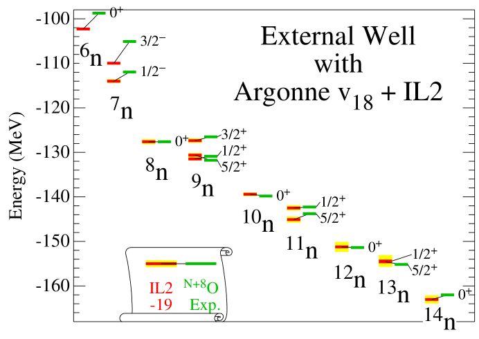
Figure 10: Energies of neutron drops compared to the corresponding oxygen isotope experimental energies.

5.5 Mimicking Oxygen Isotopes as Neutron Drops

Although GFMC is limited to light nuclei, it can be used to indirectly study large, neutron-rich, nuclei by computing neutron drops. These are collections of neutrons interacting via a realistic Hamiltonian, such as AV18+IL2, with the addition of an artificial external one-body well. The well provides the additional attraction necessary to produce a bound state of the $N$ neutrons; it can be thought of as the average effect of the protons which are not explicitly included in the calculation. Note that the $N$ neutrons occupy all shells from 0$s$ up; the well does not represent any omitted neutrons.

Figure 10 shows results for one such study in which we attempt to mimic the neutron-rich isotopes of oxygen. Here we consider that the $N$-neutron drop represents ^8+NO. The external well is of the Woods-Saxon form with parameters $R=3.0$ fm, $a=1.1$ fm, and $V=-35.5$ MeV; these were chosen in an attempt to get the correct separation energies for ^17,18O. Since the energy of the 8 protons is not included in the calculation, the energies of all the neutron drops are shifted (by 19 MeV) to match the 8-neutron drop with the experimental ¹⁶O energy. The Woods-Saxon well binds 0$s$ and 0$p$ nucleons but does not have 0$d$ or 1$s$ bound states; thus the binding of neutrons in the $sd$ shell arises from the combination of the well and the intrinsic AV18+IL2 potentials.

We see that the energies of the neutron-rich oxygen isotopes up to ²²O are reasonably well reproduced by this model. However the 9-neutron drop has a $\mbox{$\textstyle{1\over 2}$}^{+}$ ground state rather than the desired $\mbox{$\textstyle{5\over 2}$}^{+}$. It appears necessary to add a spin-orbit term to the well to achieve the correct ground state. Once a satisfactory model has been produced, the densities and other properties of these model oxygen isotopes can be studied.

6 Conclusions

Calculations with errors of only 1 to 2% of energies for nuclei from $A$ = 6 to 12 for a given Hamiltonian are now possible. The AV18+IL2 Hamiltonian gives average binding-energy errors $<0.7$ MeV for $A=3-12$. A three-nucleon potential is required to obtain sufficient binding in the $p$-shell; it is also required to reproduce many experimental spin-orbit splittings and several level orderings. The GFMC and VMC wave functions can be used to study many other nuclear properties.

References

- [1] S. C. Pieper and R. B. Wiringa, Annu. Rev. Nucl. Part. Sci. 51 (2001) 53.
- [2] S. C. Pieper, K. Varga, and R. B. Wiringa Phys. Rev. C 66 (2002) 044310.
- [3] S. C. Pieper, V. R. Pandharipande, R. B. Wiringa, and J. Carlson, Phys. Rev. C 64 (2001) 014001.
- [4] S. C. Pieper, R. B. Wiringa, and J. Carlson, Phys. Rev. C, in press.
- [5] P. Navrátil and W. E. Ormand, Phys. Rev. C 68 (2003) 034305.
- [6] S. C. Pieper, Phys. Rev. Lett. 90 (2003) 252501.
- [7] R. B. Wiringa, V. G. J. Stoks, and R. Schiavilla, Phys. Rev. C 51 (1995) 38.
- [8] J. R. Bergervoet, et al. Phys. Rev. C 41 (1990) 1435; V. G. J. Stoks., et al. Phys. Rev. C 48 (1993) 792.
- [9] B. S. Pudliner, V. R. Pandharipande, J. Carlson, and R. B. Wiringa, Phys. Rev. Lett. 74 (1995) 4396.
- [10] J. Fujita and H Miyazawa, Prog. Theor. Phys. 17 (1957) 360.
- [11] B. S. Pudliner et al., Phys. Rev. C 56 (1997) 1720.
- [12] R. B. Wiringa, S. C. Pieper, J. Carlson, and V. R. Pandharipande, Phys. Rev. C 62 (2000) 014001.
- [13] H. Kamada, et al. Phys. Rev. C 64 (2001) 044001.
- [14] S. C. Pieper and V. R. Pandharipande, Phys. Rev. Lett. 70 (1993) 2541.
- [15] D. Kurath, Phys. Rev. 101 (1956) 216.
- [16] S. A. Coon and H. K. Han, Few-Body Syst. 30 (2001) 131.
- [17] F. M. Marqués et al., Phys. Rev. C 65 (2002) 044006.
- [18] R. B. Wiringa and S. C. Pieper, Phys. Rev. Lett. 89, (2002)182501.
- [19] L.-B. Wang et al., Phys. Rev. Lett. 93 (2004) 142501.
- [20] A. E. L. Dieperink and T. de Forest, Jr., Phys. Rev. C 10 (1974) 543.