Nodal Lines in the Cranked HFB Overlap Kernels

Abstract

Norm overlap kernels of the cranked Hartree-Fock-Bogoliubov states are studied in the context of angular momentum projection. In particular, the geometrical distribution of nodal lines, i.e., one dimensional structures where the overlap kernels possess null value, is investigated in the three dimensional space defined by the Euler angles. It is important to know the distribution of these nodal lines when one attempts to determine the phase of norm overlap kernels.

The mean field approximation (MFA) is successful in the description of nuclear systems BHR03 ; Fr01 ; RS80 , to which the independent particle motion picture can be applied RS80 ; Br54 ; BG57 . Deformation and superfluidity (superconductivity) in nuclei are good examples RS80 that are explained by MFA. Although some essential correlations are taken into account through MFA in an efficient manner, it fails to incorporate other important features such as symmetries and relevant higher order correlations, which may be necessary for studying nuclear structures further BHR03 ; RS80 .

Within MFA, physical quantities such as energy and quadrupole moment are calculated as expectation values, but there is room for further quantisations. For example, angular momentum is not conserved when the rotational symmetry is spontaneously broken by deformed mean fields. As a consequence, the corresponding many-body state has the form of a wave packet IMR79 . In the cranking model Ing56 , which describes a rotating mean field in a semi-classical manner, the mean field state is written as

$$|\psi_{\rm MFA}(\omega)\rangle=\sum_{IM}C^{I}_{M}(\omega)|IM\rangle.$$ (1)

(The rotational frequency of the deformed mean field is denoted by $\omega$, while the quantum numbers for total angular momentum and its magnetic quantum number are expressed as $I$ and $M$, respectively .) $|\psi_{\rm MFA}(\omega)\rangle$ usually has large fluctuations in its probability distribution $|C^{I}_{M}|^{2}$. The width of the fluctuations becomes larger at higher spin IMR79 , which means $|\Psi_{\rm MFA}(\omega)\rangle$ possesses a more averaged character. As a consequence, a simple application of the cranking model faces difficulty, for instance, in the description of the mixture of two different states in band crossing regions Ham76 .

A quantum mechanical description of collective rotation is given in the generator coordinate method (GCM) HW52 with a choice of the Euler angles ($\Omega\equiv(\alpha,\beta,\gamma$)) as generator coordinates. This method corresponds to angular momentum projection (AMP) PY57 . Rotational symmetry spontaneously broken by the deformed mean field can be restored by superposing the states that point various orientations $|\psi(\Omega)\rangle\equiv\hat{R}(\Omega)|\psi_{\rm MFA}\rangle$ . ( $\hat{R}(\Omega)$ is a rotational operator in the three dimensional space. See Eq.(13) below.) A state with symmetry restoration $|\Phi\rangle$ is schematically expressed as

$$|\Phi\rangle=\int d\Omega f(\Omega)|\psi(\Omega)\rangle,$$ (2)

with $f(\Omega)$ being the weight function that is determined by the variational principle. This state $|\Phi\rangle$, a superposition of the infinite number of degenerate states, corresponds to a Nambu-Goldstone mode NG60 in a finite system.

In our previous works, we have numerically performed AMP in attempts to describe high-spin states, such as tilted rotation for high-$K$ states in ¹⁷⁸W OWA02 and the wobbling motion in the multi-band crossing region in ¹⁸²Os OAHO00 . Through these works, we found it difficult to perform numerical calculations of AMP in some situations. Such situations are observed to occur, for example, in the calculations of AMP applied to cranked HFB states at high spin (angular momentum ranging from $10$ to $20\hbar$). A typical problem is negative values of the probability $|C^{I}_{M}|^{2}$ for $I$ being odd integer, although the probabilities for even $I$ seem reasonably calculated . (See Fig.1.)

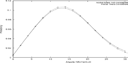
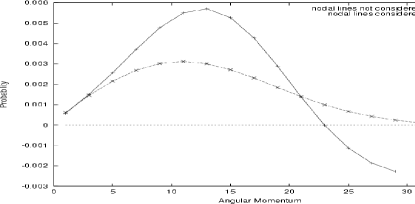
Even-$I$	Odd-$I$.

Figure 1: Probability distributions of angular momentum using two types of prescription to determine the sign of the norm overlap kernels. The solid line represents the probability obtained by the old method while the dashed line is by the new method. The constraint value on angular momentum is $J=14\hbar$. The left (right) panel shows even-$I$ (odd-$I$) components. Note the different scales in the first and second panels.

We first suspected the coarse mesh employed in the numerical integration causes this difficulty, because the integration in the AMP formula (See Eq.(9) below) is discretised in numerical calculations with respect to the Euler angles. The appropriate mesh size can be estimated by using the uncertainty principle $\Delta I\Delta\Omega\simeq\hbar$. The constraint value $\langle\hat{J}_{1}\rangle=J$ and the fluctuation $\Delta I$ are roughly related as $\Delta I\simeq J/2$ at high spin IMR79 ; OOTH98 . Then, $\Delta\Omega=2\hbar/J$. For example, $\Delta\Omega\simeq 6^{\circ}$ for $J=20\hbar$. The appropriate number of mesh points are therefore about 60 for $\alpha,\gamma,$ and 30 for $\beta$. Even with this mesh size, however, the problem was observed to occur in performing AMP when high spin states are considered (i.e.,$J>10\hbar$). On the other hand, when the angular momentum is low ($J\leq 10\hbar$), AMP is successfully performed, as expected.

We then suspect that the poor determination of the sign of the norm overlap kernels, which will be given in Eq.(14), may cause this problem. These kernels are necessary in the AMP procedure, in which the state in the projected space is expressed as

$$|\Psi^{I}_{M}\rangle=\sum_{K}g^{I}_{K}\hat{P}^{I}_{MK}|\psi_{\rm MFA}\rangle.$$ (3)

The coefficients $g^{I}_{K}$ are determined by a variational equation

$$\sum_{K}\left(H^{I}_{MK}-E^{I}N^{I}_{MK}\right)g^{I}_{K}=0.$$ (4)

Here, $\hat{P}^{I}_{MK}$ denotes the AMP operator, and matrices $N^{I}_{MK}$ and $H^{I}_{MK}$ are defined as,

$$\left(\begin{array}[]{c}N^{I}_{MK}\\ H^{I}_{MK}\end{array}\right)=\langle\psi_{\rm MFA}|\left(\begin{array}[]{c}\hat{P}^{I}_{MK}\\ \hat{H}\hat{P}^{I}_{MK}\end{array}\right)|\psi_{\rm MFA}\rangle$$ (9)

$$= \!\!\frac{2I+1}{8\pi^{2}}\!\!\int\!\!d\Omega D^{I*}_{MK}(\Omega)\langle\psi_{\rm MFA}|\left(\begin{array}[]{c}\hat{R}(\Omega)\\ \hat{H}\hat{R}(\Omega)\end{array}\right)|\psi_{\rm MFA}\rangle.$$ (12)

A useful relation to note here is $|C^{I}_{M}|^{2}=N^{I}_{MM}$. The measure in the three-dimensional Euler space $d\Omega$ is defined as $d\alpha\sin\beta d\beta d\gamma$, and the integration intervals are $\left[0,2\pi\right]$ for $\alpha$ and $\gamma$, and $\left[0,\pi\right]$ for $\beta$. The rotational operator $\hat{R}(\Omega)$ is given as

$$\hat{R}(\Omega)=\exp(-i\alpha\hat{J}_{z})\exp(-i\beta\hat{J}_{y})\exp(-i\gamma\hat{J}_{z}).$$ (13)

The quantities $\langle\psi_{\rm MFA}|\hat{R}(\Omega)|\psi_{\rm MFA}\rangle$ and $\langle\psi_{\rm MFA}|\hat{H}\hat{R}(\Omega)|\psi_{\rm MFA}\rangle$ in Eq.(9) are called norm and energy overlap kernels, respectively. They are calculated through formulae derived by Onishi et al OY65 ; OH80 . By utilising the Onishi formulae, one can calculate the norm overlap kernel as

$$N(\Omega)=\langle\psi_{\rm MFA}|\hat{R}(\Omega)|\psi_{\rm MFA}\rangle=\sigma(\Omega)\sqrt{{\rm det}P(\Omega)},$$ (14)

where $\sigma(\Omega)$ has values $\pm 1$. This ambiguity in sign comes from the square root operation. We will come back to this point shortly. The matrix $P(\Omega)$ is written OH80 ,

$$P(\Omega)=U^{{\dagger}}D^{{\dagger}}(\Omega)U+V^{{\dagger}}D^{T}(\Omega)V,$$ (15)

where $U$ and $V$ are matrices defined in the general Bogoliubov transformation RS80 between canonical ($c_{\mu}\ c^{{\dagger}}_{\mu}$) and quasi-particle annihilation and creation operators $(\beta_{i}\ \beta^{{\dagger}}_{i}$):

$$\left(\begin{array}[]{c}\beta_{i}\\ \beta_{i}^{{\dagger}}\end{array}\right) = \left(\begin{array}[]{cc}U_{\mu i}^{*}&V_{\mu i}^{*}\\ V_{\mu i}&U_{\mu i}\end{array}\right)\left(\begin{array}[]{c}c_{\mu}\\ c_{\mu}^{{\dagger}}\end{array}\right).$$ (22)

The presence of $\sigma(\Omega)$ implies that ${N}(\Omega)$ is a two-valued function of $\Omega$ although it should be physically well-defined and single-valued. Therefore, it is necessary to choose an appropriate sign for given $\Omega$. Two methods have been proposed HHR82 ; NW83 to determine the sign of $\sigma(\Omega)$, but due to its numerical feasibility the method of Hara, Hayashi and Ring HHR82 is widely used. It makes use of the continuity of the norm overlap kernel as a function of the Euler angles $\Omega$. Our calculations are based on this method, and the procedure is explained below.

First of all, the origin in the Euler space is assumed to have some certain phase. (In our case, $\sigma(0)=+1$.) Then, by analytical continuation, the well-defined region is extended until the whole Euler space is covered. To achieve this, the Euler space is divided into domains defined as follows: Writing $N(\Omega)=r(\Omega){\rm e}^{i\theta(\Omega)}$, the argument $\theta(\Omega)$ and the norm $r(\Omega)$ are supposed to be continuous with respect to $\Omega$. Then, a point $\Omega=\Omega(\alpha,\beta,\gamma)$ belongs to a domain $D_{n}\ (n=0,\pm 1,\pm 2,\cdots)$ when $(n-\frac{1}{2})\pi<\theta(\Omega)\leq(n+\frac{1}{2})\pi$. Inside each domain, $\sigma(\Omega)$ is determined to be $+1$ for even $|n|$ and $-1$ for odd $|n|$. The boundary between $D_{n}$ and $D_{n+1}$ is determined by tracking the continuity of $\theta(\Omega)$ through the derivative information. In this way, ${N}(\Omega)$ becomes well-defined as a single-valued function in the entire domain $D\equiv\bigcup_{n}D_{n}$ (i.e., the whole Euler space) .

As mentioned above, derivatives of the norm overlap kernels are used to check the continuity of $\theta(\Omega)$. A set of formula derived by Onishi et al. is again useful to calculate these derivatives OH80 , which are now given in the form of logarithmic derivatives,

$$\frac{\partial}{\partial\Omega}\ln\langle\psi_{\rm MFA}|\hat{R}(\Omega)|\psi_{\rm MFA}\rangle=\frac{1}{2}\frac{1}{{\rm det}P(\Omega)}\frac{\partial}{\partial\Omega}{\det}P(\Omega).$$ (23)

Detailed forms for the formulae are given in Ref.OH80 . (Sometimes the formulae are called generalised Wick’s theorem RS80 .) Because the argument of the norm overlap kernel is written as,

$$\theta(\Omega)={\rm Im}\left[\ln\langle\psi_{\rm MFA}|\hat{R}(\Omega)|\psi_{\rm MFA}\rangle\right],$$ (24)

the derivatives of $\theta(\Omega)$ can be computed through Eq.(23). Note that the derivative of the argument, $\theta^{\prime}=\frac{\partial\theta}{\partial\Omega}$, is uniquely evaluated , i.e., being free from the sign ambiguity, because these formulae essentially make use of the square of the norm overlap kernels (${N}(\Omega)^{2}$) to eliminate the ambiguity coming from $\sigma(\Omega)$.

To specify the domain $D_{n}$, we consider the following two quantities that can be calculated from a pair of neighbouring mesh points displaced by small distance $\Delta\Omega$, that is, (i) the difference between the two points, corresponding to the approximate derivative of the argument $\theta(\Omega)$ obtained by the two-point formula, which is

$$a(\Omega)\equiv\frac{\theta(\Omega+\Delta\Omega)-\theta(\Omega)}{\Delta\Omega}$$ (25)

and (ii) the average of $\theta^{\prime}$ obtained through Eq.(23) between the two points, which is

$$b(\Omega)\equiv\frac{\theta^{\prime}(\Omega+\Delta\Omega)+\theta^{\prime}(\Omega)}{2}.$$ (26)

Note that only $a(\Omega)$ suffers from the sign ambiguity, but $b(\Omega)$ does not. We can now determine the relative sign of the kernel between the points $\Omega$ and $\Omega+\Delta\Omega$ by checking the magnitude of the residue $\delta\theta(\Omega)\equiv a(\Omega)-b(\Omega)$. When the value of the residue is small, or behaves as $\delta\theta(\Omega)\simeq-\frac{\theta^{(3)}(\bar{\Omega})}{12}\Delta\Omega^{2}$ with $\Omega<\bar{\Omega}<\Omega+\Delta\Omega$, the neighbouring point $\Omega+\Delta\Omega$ is judged to be in the same domain $D_{n}$ as the reference point $\Omega$. On the contrary, the point $\Omega+\Delta\Omega$ belongs to the different domain if the following two conditions are satisfied: (i) $\delta\theta$ returns a significant deviation from the behaviour of $-\frac{\theta^{(3)}(\bar{\Omega})}{12}\Delta\Omega^{2}$; and (ii) the deviation is removed after the sign $\sigma(\Omega+\Delta\Omega)$ is inverted and the resultant residue follows the behaviour of $-\frac{\theta^{(3)}(\bar{\Omega})}{12}\Delta\Omega^{2}$.

According to the results in our calculations, the above naive approach works for $J\leq 10\hbar$, but it seems to fail when high spin states are considered ($J>10\hbar$). A typical symptom of the failure is seen as violation of the positive definite nature in probability, as illustrated in the right portion of Fig.1. In Fig.1, angular momentum components in the cranked HFB states at $J=14\hbar$ are plotted, that is,

$$W^{I}\equiv\text{Tr}(N^{I})=\sum_{M=-I}^{I}|C^{I}_{M}(\langle\hat{J}_{1}\rangle=14\hbar)|^{2},$$ (27)

where the matrix $N^{I}$ is defined in Eq.(9) and the trace is taken with respect to the magnetic quantum number $M$. With the above method to determine the sign (solid lines in the figure), AMP seems to work properly when the even-$I$ distribution of $W^{I}$ is concerned (i.e., the left portion in the figure), while in the right portion the positive definite nature of $W^{I}$ is violated slightly to an order of magnitude of $10^{-3}$. One may say that such small numerical errors can be neglected when proper physics is extracted from the results. In fact, as far as the ground state rotational bands are concerned (which consist of only even-$I$ components), it may be justified to ignore these small errors. However, we would like to investigate the cause of the errors in this paper because high-spin physics involving odd-$I$ states (e.g., high-$K$ bands) becomes more and more important today.

The above problem (i.e., negative probability) implies that the resultant norm overlap kernels do not satisfy proper features as a physical quantity. A possible reason for this defect is the assumption of the continuity of $\theta(\Omega)$. It is, in fact, singular on a nodal line, i.e., a set of points where the norm overlap kernel becomes zero ($r(\Omega)=0$). The analytical continuation approach assumes the continuity of norm overlap kernels (more precisely, of the argument $\theta(\Omega)$), so that the method fails to work in the neighbourhood of nodal lines.

To deal with the nodal lines in the context of the sign determination, there are basically two approaches. One is to find out all the nodal lines in the Euler space (from the information of $r(\Omega)=0$). Once the locations of the nodal lines are known, one can determine $\sigma(\Omega)$ without any ambiguity because we can avoid the calculations of the residue $\delta\theta$ between two points sandwiching the nodal lines. The other is to calculate the residues for all the possible directions (that is, $\Delta\Omega=$$\pm\Delta\alpha$, $\pm\Delta\beta$, and $\pm\Delta\gamma$) no matter where the nodal lines are. In this case, optimisation regarding to the values of the residues is made by fixing $\sigma(\Omega+\Delta\Omega)$ in a manner of trial-and-error. In this paper, the second approach is chosen for the sake of simplicity in numerical calculations.

Although there is no need to know explicit information about the geometry and topology of the nodal lines in the present approach, we realise that such information are very useful to clarify the nature and source of the problem. Therefore, in this paper, we try to pin down the locations of nodal lines, and succeed to find them for the first time. (Figs.2 and 3).

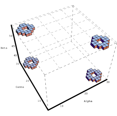
(A) $\Delta\alpha=\Delta\gamma=10^{\circ}$, and $\Delta\beta=2^{\circ}$.

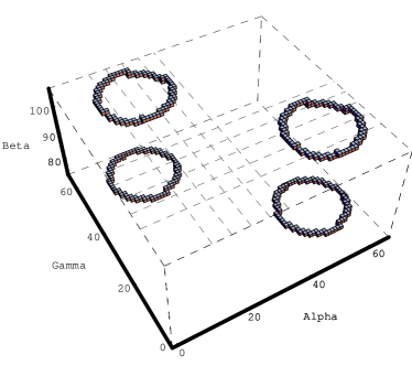
(B)$\Delta\alpha=\Delta\gamma=5^{\circ}$, and $\Delta\beta=1^{\circ}$.

Figure 2: Nodal lines at $J=12\hbar$ with low and high resolutions for the mesh size.

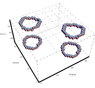
(A) $\Delta\alpha=\Delta\gamma=10^{\circ}$, and $\Delta\beta=2^{\circ}$.

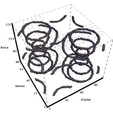
(B) $\Delta\alpha=\Delta\gamma=5^{\circ}$, and $\Delta\beta=1^{\circ}$.

Figure 3: Nodal lines at $J=14\hbar$ with low and high resolutions for the mesh size. The detailed structure of (B) is shown in Fig.4.

Let us first discuss the nodal lines we found, before the detailed explanation is given on the new method to determine the sign $\sigma$. To obtain norm overlap kernels, we first perform principal axis cranked HFB calculations with a constraint on angular momentum $\langle\hat{J}_{1}\rangle\equiv J$ (as well as constraints on particle numbers). The pairing-plus-Q$\cdot$Q force is employed with the standard choices for the force parameters and model space BK65 . This HFB calculation is performed in a fully self-consistent manner, so that the gamma (triaxial) deformation is self-consistently handled. The details of the method used for this calculation are explained in Ref.HO96 . Then, as already mentioned above, the overlap kernels are obtained by means of the Onishi formulae such as Eqs. (14) and (23). The modified method for the phase determination, which will be explained later, is employed to calculate the norm overlap kernels. ¹⁷⁰Dy is chosen in this study, as a well-deformed rare-earth nucleus. ($\beta=0.295,\Delta_{p}=0.867$ (MeV), $\Delta_{n}=0.652$ (MeV) at $J=0$ MN .) The yrast line of this nucleus does not show any crossings at high spin ($\leq 20\hbar$) in our calculation. (The more complicated structure of nodal lines may appear in the cranked HFB states in band-crossing regions. Such states are planned to be studied in future.)

Figs.2 and 3 present the nodal lines found in cranked HFB states at $J=12\hbar$ and $14\hbar$, respectively. In the figures, cubes are used to show and cover the regions where nodal lines exist, for graphical convenience. The size of the cubes is the same as the mesh size used in AMP. It is given by $\Delta\Omega=L_{\Omega}/N_{\Omega}$, where $L_{\alpha}=L_{\gamma}=2\pi$ and $L_{\beta}=\pi$. The number of the mesh points are $N_{\alpha}=N_{\gamma}=36\ (72)$ and $N_{\beta}=90\ (180)$ for the low (high) resolution calculations.

The positions of nodal lines are determined in the following approximation: on each face of the cube, after the phase determination, the norm kernels are linearly interpolated with respect to the Euler angles, that is,

$${N}_{\text{linear}}(\Omega)\simeq c_{1}\alpha+c_{2}\beta+c_{3}\gamma+c_{4}.$$ (28)

The coefficients $c_{i}$ are determined by the exact values of ${N}(\Omega)$ at the four vertices on the face. The position of the nodal line on the face is obtained by solving the simultaneous equations of

$$\text{Re}[{N}_{\text{linear}}]=\text{Im}[{N}_{\text{linear}}]=0.$$ (29)

In the present study, no nodal lines are found in $0\leq J\leq 10\hbar$. Nodal lines are found in $12\hbar\leq J\leq 20\hbar$ and form a simple topology of closed loops (rings) without knots. Their geometrical distributions seem to become more complicated as the value of $J$ becomes larger. It is seen in Fig.3 that some of the nodal lines are missing in the low resolution calculation but this result is due to the simple linear approximation, Eq.(28), for the complicated geometrical distribution of the nodal lines.

Symmetries seen in Figs.2 and 3, are expressed by

$$\langle\hat{R}(\alpha,\beta,\gamma)\rangle=\langle\hat{R}(\gamma,\beta,\alpha)\rangle^{*}$$ (30)

$$= \!\!\langle\hat{R}(\pi-\alpha,\pi-\beta,\gamma)\rangle^{*}\!\!=\!\!\langle\hat{R}(\alpha,\pi-\beta,\pi-\gamma)\rangle^{*}$$ (31)

$$= \langle\hat{R}(\alpha+2\pi,\beta,\alpha)\rangle=\langle\hat{R}(\alpha,\beta,\gamma+2\pi)\rangle.$$ (32)

and are attributed to the properties possessed by the principal-axis cranked HFB states HHR82 such as the signature.

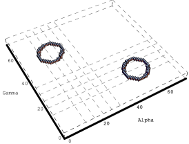
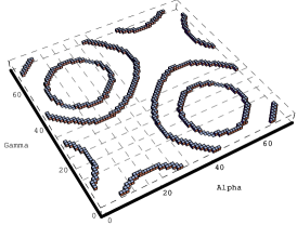
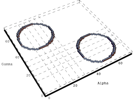
(a)  $\beta\simeq 100^{\circ}$	(b)  $\beta\simeq 110^{\circ}$	(c)  $\beta\simeq 120^{\circ}$

Figure 4: Detailed pictures of the essential nodal rings in Fig.3(B) with respect to $\beta$.

As a result of these symmetries (especially, Eqs. (30) and (31)), there are four identical sets of nodal lines in Figs.2 and 3. In other words, there is essentially only one nodal line (ring) out of the four shown in Figs.2 and 3(A), while there are sixteen nodal rings in Figs.3(B) but just four of them are essential. Two out of these four essential rings form a concentric circles, as shown in the second portion of Fig.4(b). (Note the symmetry on the boundary is given in Eqs.(32).) Although these rings look to be completely two-dimensional, that is, confined in the constant $\beta$ plane, one can tell their three-dimensional structure with a careful look at the figures.

Let us now explain the details of the new approach to determine the sign $\sigma(\Omega)$ below. First of all, the third order derivatives of the norm overlap kernels are chosen to be a measure of the “smoothness” of the kernels. In fact, such a quantity is practically easily computed in our calculations where the norm overlap kernel and its first order derivatives are already obtained. Using the Taylor expansions for $N(\Omega+\Delta\Omega)$ and $\frac{\partial N(\Omega+\Delta\Omega)}{\partial\Omega}$, the third derivative between two points $\Omega$ and $\Omega^{\prime}=\Omega+\Delta\Omega$ is approximately obtained up to an order of ${\cal O}(\Delta\Omega)$, which is denoted here as $D_{3}(\Omega^{\prime},\Omega)$,

$$D_{3}(\Omega^{\prime},\Omega) = \frac{6}{(\Delta\alpha)^{2}}\left\{\frac{\partial N}{\partial\alpha}(\Omega^{\prime})+\frac{\partial N}{\partial\alpha}(\Omega)\right\}$$

$$- \frac{12}{(\Delta\alpha)^{3}}\left\{N(\Omega^{\prime})-N(\Omega)\right\}.$$

The above expression corresponds to a case when two points are displaced along the $\alpha$ coordinate, i.e., $\Omega=(\alpha,\beta,\gamma)$ and $\Omega^{\prime}=(\alpha+\Delta\alpha,\beta,\gamma)$. Similar expressions hold for a pair of adjacent points displaced in the $\beta$ or $\gamma$ direction. Note that $D_{3}$ is a complex quantity in contrast to the residue $\delta\theta$, which is a real quantity. An advantage to extend the residue $\delta\theta$ to the complex $D_{3}$ is that the continuity is checked not only by $\theta(\Omega)$ but also by $r(\Omega)$. $D_{3}$ is particularly useful in the vicinity of the nodal lines where $\ln r(\Omega)$ diverges so quickly. In this case, $\delta\theta$ can also change rapidly to return the large value as if the boundary of domains appeared to be detected. With all the available information on the continuity both in the norm and argument, the boundary between domains $D_{n}$ and $D_{n+1}$ is determined with more certainty even in the vicinity of the nodal lines. Next, starting from $\Omega=(0,0,0)$, where $\sigma=1$ is assumed, we determine one by one the sign of $\sigma$ for the adjacent mesh points so that $|D_{3}|$ takes a smaller value. As we proceed, conflicting assignments in sign are seen for a point $\Omega=(\alpha,\beta,\gamma)$. In other words, when $D_{3}$ is evaluated along two different links, say links between $\Omega$ and $\Omega+\Delta\Omega=(\alpha\pm\Delta\alpha,\beta,\gamma)$, the signs at $\Omega$ are sometimes inconsistent. In this case, we use “reliability” to decide which sign assignment has priority. Although there is no unique way to define the “reliability”, our choice for the definition is the ratio of $|D_{3}|$ between the sign-flipped and unflipped cases (the smaller value should be in the denominator): larger values of this ratio indicate more reliability. This procedure is performed for all the links and optimisation on $D_{3}$ is carried out. The whole optimisation procedure is repeated many times until the average reliability is converged. The essential point in this new method is that we attempt to proceed with the analytical continuation through the only links where a reliable determination of the relative sign seems possible. With this requirement, many problematic points like those near the nodal lines are circumvented or isolated from the analytical continuation procedure.

Figure 5: Probability distributions for $J=12\hbar$ - $20\hbar$ with the modified phase determination method. The upper (lower) panel shows the profile for even-$I$ (odd-$I$) components.

This new method is quite powerful especially when one attempts to determine the sign of norm overlap kernels in the presence of the nodal lines. An advantage of the method is that we do not need to find the nodal lines explicitly. To confirm the advantage, we analysed where the disagreements in the sign determination happen between the previous naive method (in which the signs are determined one by one in a scheduled simple order along straight lines) and the present new method. We then found that the discrepancies are concentrated in the vicinity of regions where nodal lines exist. The improvement in the sign determination by the new method is clearly demonstrated in Fig.1 as the recovery of the positive definiteness of the probability in the odd-$I$ distributions of $W^{I}$. A disadvantage of this new method is that it is more time-consuming than the previous method. However, we found that the computation time has been greatly improved with the combination of the two methods: the initial sign determination is made by the first naive approach and subsequently the new optimisation method is carried out.

In the case of ¹⁷⁰Dy, we have checked that this newly developed method improves the sign determination up to $J=14\hbar$. Although several doubtful sign assignments start to occur at $J=16\hbar$ even for the higher resolution, these potential mistakes do not seem to affect positive definiteness in probabilities ($|C^{I}_{M}|^{2}\geq 0$) and the sum rule,

$$\sum_{I=0}W^{I}=1,$$ (34)

up to $J=20\hbar$. In Fig.5, the results of the modified probability distributions are plotted. The integrals of each probability distribution curve, i.e., the probability sum rule, are presented in Table 1.

$J\equiv\langle\hat{J}_{1}\rangle_{\rm HFB}$	$12\hbar$	$14\hbar$	$16\hbar$	$18\hbar$	$20\hbar$
$P$	0.998	0.991	0.981	0.965	0.939

Table 1: The total probability sum $\displaystyle P=\sum_{I<35\hbar}W^{I}$ shown in Fig.5.

$W^{I}$ satisfies the sum rule quite well up to $I=34\hbar$. The problem of negative probability does not appear until $I=31\hbar$. Beyond $I=31\hbar$ for the odd-$I$ components (and beyond $I=34\hbar$ for the even-$I$), all $W^{I}$ become negative. The reason for this behaviour is attributed to the discretisation approximation in the integration. With $\Delta\alpha=\Delta\gamma=5^{\circ}$ and $\Delta\beta=1^{\circ}$, the integration in angular momentum projection manages to be valid up to

$$I\simeq\frac{1}{3}\left(\frac{2\hbar}{\Delta\alpha}+\frac{2\hbar}{\Delta\beta}+\frac{2\hbar}{\Delta\gamma}\right)=32\hbar.$$ (35)

The divergence in the curves of $J=12\hbar$ (beyond $I>34\hbar$ for the even-$I$ graph and $I>33\hbar$ for odd-$I$) comes from the same reason. To overcome even these difficulties, a finer mesh size should be employed. Such a line of investigation is now in progress.

In conclusion, we have studied the distribution of zeros of norm overlap kernels of cranked HFB states. Such zeros form one dimensional structure in the three-dimensional space defined by the Euler angles, so that we call it a “nodal line”. The existence of nodal lines is numerically demonstrated for the first time, and we have found they emerge as spin increases and their structure becomes more complicated as angular momentum becomes larger ($J>10\hbar$). We have shown that it is important to know the distributions in order to correct wrong assignments for the sign of norm overlap kernels. The correction is essential for angular momentum projection to be performed with high accuracy for cranked mean-field states.

- (1) M. Bender, P.-H. Heenen, P.-G. Reinhard, Rev. Mod. Phys. 75, 121 (2003).
- (2) S. Frauendorf, Rev. Mod. Phys. 73, 463 (2001).
- (3) P. Ring, P. Schuck, The Nuclear Many-body Problem (Springer-Verlarg, Berlin, 1980).
- (4) K. A. Brueckner, Phys. Rev. 97, 1353 (1955).
- (5) H. A. Bethe, J. Goldstone, Proc. Roy. Soc. A238, 551 (1957).
- (6) S.Islam, H.J.Mang, P.Ring, Nucl. Phys. A326, 161 (1979); p.483 in Ref. RS80 .
- (7) D. R. Inglis, Phys. Rev. 103, 1786 (1956); p.126 in Ref. RS80 .
- (8) I. Hamamoto, Nucl. Phys. A271, 15 (1976).
- (9) D. L. Hill, J. A. Wheeler, Phys. Rev. 89, 106 (1952); p.398 in Ref. RS80 .
- (10) R. E. Peierls and J. Yoccoz, Proc. Phys. Soc. A70, 381 (1957); p.473 in Ref. RS80 .
- (11) Y. Nambu, Phys. Rev. Lett. 4, (1960) 380; Y. Nambu and G. Jona-Lasinio, Phys. Rev. 122, (1961) 345; J. Goldstone, Nuovo cimento 19, (1961) 154.
- (12) M. Oi, P.M.Walker, A.Ansari, Phys. Lett. B525, 255 (2002).
- (13) M. Oi, A.Ansari, T.Horibata, N.Onishi, Phys. Lett. B480, 53 (2000).
- (14) M. Oi, N. Onishi, N. Tajima, T. Horibata, Phys. Lett. B418, 1 (1998).
- (15) N. Onishi and S. Yoshida, Nucl. Phys. 80, 367 (1966); or see p.618 in Ref.RS80 .
- (16) N. Onishi, T. Horibata, Prog. Theor. Phys. 64, 1650 (1980).
- (17) K. Hara, A. Hayashi, P. Ring, Nucl. Phys. A385, 14 (1982).
- (18) K.Neergård, E.Wüst, Nucl. Phys. A402, 311 (1983).
- (19) M. Baranger, K. Kumar, Nucl. Phys. 62, 113 (1965); K. Kumar, M. Baranger, Nucl. Phys. A110, 529 (1968).
- (20) T. Horibata, N. Onishi, Nucl. Phys. A 596, 251 (1996).
- (21) P. Möller, J. R. Nix, W. D. Myers, and W. J. Swiatecki, Atomic Data Nucl. Data Tables 59, 185 (1995).