Abstract

The productions of muon pairs from the decay of heavy quarkonia have been evaluated for different centrality of the nuclear collisions at LHC energies. The effects of the various comover scenarios on the survival probability of the heavy quarkonia have been considered. The effects of shadowing and comover suppressions on the dilepton spectra originating from the decays of $J/\psi$ is found to be substantial. The dilepton yield from the thermal $J/\psi$ has also been estimated and found to be small.


Charmonium at LHC: Production, Propagation and Decay

Pradip Roya111Part of the work has been done at CERN Theory Division, CERN, Geneva, Abhee K. Dutt-Mazumdera, Jane Alamb, and Bikash Sinhaa,b a) Saha Institute of Nuclear Physics, 1/AF Bidhan Nagar, Kolkata, India

b) Variable Energy Cyclotron Centre, 1/AF Bidhan Nagar, Kolkata, India

I. Introduction

Ever since the possibility of creating quark gluon plasma (QGP) in relativistic heavy ion collision was envisaged, numerous signals were proposed to probe the properties of such an exotic state of matter. In this context Satz and MatsuiΒ [1] had suggested that the production of heavy quark resonances ($J/\psi$) will be suppressed as a result of colour Debye screening in a hot and dense system of quarks, anti-quarks and gluons. This suppression could be detected experimentally through the dileptonic decay mode of these resonances. ALICE dimuon spectrometerΒ [2] is dedicated to look for this type of signal. However, it is a daunting task to disentangle the contributions of the heavy quarkonium states to muon spectrum due to the background from several other sources, e.g. Drell-Yan, semileptonic decay of open heavy flavoured mesons ($D{\bar{D}},B{\bar{B}}$) etc. Low energy muons from kaons and pions also constitute a large background.

In this work we shall estimate the dimuon production from the decay of both hard (i.e. $J/\psi$ produced from initial hard process, will be called hard $J/\psi$ hereafter) and thermal $J/\psi$’s. In heavy ion collisions the production and decay of hard $J/\psi$ or $\Upsilon$ proceeds through the following three steps: (i) the production of pair of heavy quarks (perturbative), (ii) their resonance interactions to form the bound state (non-perturbative) and (iii) the propagation of the quarkonia through the medium and their subsequent decay to dileptonic modes with certain branching ratios.

The initial state in relativistic heavy ion collisions consists of either hadronic matter or QGP depending on the incident energies of the colliding nuclei. At LHC energies the formation of QGP is almost unavoidable. Even if the system is formed in QGP phase it will revert back to hadronic phase due to the cooling of the expanding QGP system and hence the interaction of the $J/\psi$ formed in initial hard collision with the hadronic matter is inevitable. Therefore,, we need to consider the survival probability of those $J/\psi$ due to its interactions with the hadronic medium.

At high temperatures a non-negligible number of $J/\psi$ mesons is expected in the thermal medium, which decay to lepton pair. The dilepton spectra originating from these thermal $J/\psi$ is also estimated here.

The paper is organized as follows. In section II we shall describe the formalism for the production, propagation and decay of hard and thermal $J/\psi$’s. In section III results of our calculations will be presented followed by summary and discussion in section IV.

II. Production, Propagation and Decay of Hard and Thermal $J/\psi$

a. Production

In this section we shall consider the hard $J/\psi$ production in the colour evaporation model (CEM)Β [3] and their decays to lepton pairs. As mentioned before this consists of two stages: (i) production of a $c{\bar{c}}$ pair (perturbative process) and (ii) subsequent non-perturbative evolution into asymptotic states. We have considered those hard processes which can contribute to $c\bar{c}$ productions irrespective of their colour and spin-parity. The colour neutralization occurs by the interactions (one or more soft gluon emission) with the surrounding colour fields and this step is considered to be non-perturbative. In CEM quarkonium production is treated identically to open heavy flavour production with the exception that in the case of quarkonium, the invariant mass of the heavy quark pair is restricted below the open meson threshold, which is twice the mass of the lowest meson mass that can be formed with the heavy quark. Depending on the quantum numbers of the initial $Q{\bar{Q}}$ pair and the final state quarkonium, a different matrix element is needed for the resonance production. The effects of these non-perturbative matrix elements are combined into the universal factor $F[nJ^{PC}]$ which is a process and kinematics independent quantityΒ [4]. It describes the probability that the $Q{\bar{Q}}$ pair forms a quarkonium of given spin ($J$), parity ($P$) and charge conjugation ($C$). The production cross section for a $J/\psi$ or $\Upsilon$ is therefore given byΒ [4]

$$\sigma[R(nJ^{PC})]=F[nJ^{PC}]\,{\tilde{\sigma}}[Q{\bar{Q}}],$$ (1)

where the non-perturbative (long distance) factor can be written in terms of the probability to have colour singlet state (1/9) and the fraction $\rho_{R}$ of each specific charmonium state. The perturbative contribution (short distance) is given by

$${\tilde{\sigma}}[Q{\bar{Q}}]=\int_{2m_{Q}}^{2m_{D/B}}\,dM_{Q{\bar{Q}}}^{2}\,\frac{d\sigma[Q{\bar{Q}}]}{dM_{Q{\bar{Q}}}^{2}}.$$ (2)

The contributions to heavy quark production in leading order come from $q\,{\bar{q}}\,\rightarrow\,Q\,{\bar{Q}}$ and $g\,g\,\rightarrow\,Q\,{\bar{Q}}$. The differential cross-section for heavy flavour production in hadron-hadron collision is given byΒ [5]

$$\frac{d\sigma}{dM_{Q{\bar{Q}}}^{2}dy}[h_{A}h_{B}\rightarrow Q{\bar{Q}}X]=\frac{H(x_{a},x_{b},Q^{2})}{s},$$ (3)

where

$\displaystyle H(x_{a},x_{b},Q^{2})$ $\displaystyle=$ $\displaystyle\sum_{f}\,\left[\frac{}{}q_{f}^{h_{A}}(x_{a},Q^{2}){\bar{q}}_{f}^{h_{B}}(x_{b}.Q^{2})+\frac{}{}{\bar{q}}_{f}^{h_{A}}(x_{a},Q^{2})q_{f}^{h_{B}}(x_{b},Q^{2}){\hat{\sigma}}_{q{\bar{q}}\rightarrow Q{\bar{Q}}}\right]$ (4)
$\displaystyle+g^{h_{A}}(x_{a},Q^{2})g^{h_{B}}(x_{b},Q^{2}){\hat{\sigma}}_{gg\rightarrow Q{\bar{Q}}}.$

$x_{a,b}=M\,e^{\pm y}/\sqrt{s}$, $\sqrt{s}$ being the centre of mass energy of the hadronic system. $q_{f}$’s and $g$’s are the parton distribution functions (PDF) to be taken from CTEQ, MRST or GRVΒ [6]. Combining eqs.(1),(2) and (3) we obtain the cross-section for resonance production per unit rapidity as,

$$\frac{d\sigma}{dy}[h_{A}h_{B}\rightarrow RX]=\frac{\rho_{R}}{9}\,\int_{2m_{Q}}^{2m_{D/B}}\,dM_{Q{\bar{Q}}}^{2}\frac{H(x_{a},x_{b},M_{Q{\bar{Q}}}^{2})}{s}.$$ (5)

We take $\rho_{R}$ = 0.5 (0.207) for $J/\psi$ ($\Upsilon$).

Next we consider $J/\psi(\Upsilon)$ production in $p-A$ and $A-B$ collisions. To this end we first briefly mention the necessary formulae in Glauber modelΒ [7, 8] The total inelastic cross-section in $A-B$ collisions at an impact parameter $b$ is given by

$$\frac{d\sigma_{\mathrm{in}}^{AB}}{d\vec{b}}=1-\left[\frac{}{}1-T_{AB}(\vec{b})\,\sigma_{\mathrm{in}}^{NN}\right]^{AB}\equiv\,1-P_{0}(b),$$ (6)

where $T_{AB}(b)$ is the nuclear overlap function given by

$$T_{AB}(b)=\int\,d^{2}s\,T_{A}(b)\,T_{B}(|\vec{b}-\vec{s}|)$$ (7)

The nuclear thickness functions are normalized to unity, i. e. $\int\,d^{2}b\,T_{A}(b)=\int\,d^{2}b\,dz\,\rho_{A}(b,z)=1$

Generally we are interested in the cross-sections for a set of events in a given centrality range defined by the trigger settings. Centrality selection corresponds to a cut on the impact parameter $b$ of the collisions. The sample of events in a given centrality range $0\leq b\leq b_{m}$, contains a fraction of the total inelastic cross-section. This fraction is defined by

$\displaystyle f(b_{m})$ $\displaystyle=$ $\displaystyle\frac{\int_{0}^{b_{m}}d{\vec{b}}\,\frac{d\sigma_{\mathrm{in}}^{AB}}{d\vec{b}}}{\int_{0}^{\infty}\,d\vec{b}\,\frac{d\sigma_{\mathrm{in}}^{AB}}{d\vec{b}}}$ (8)

Now we discuss the $J/\psi$ survival probability when it propagates through the hot hadronic medium produced in nucleus-nucleus collisions. After creation the $J/\psi$ meson can interact with other nucleons in the target and the projectile and may get destroyed mainly due to $J/\psi-N$ interactions. The cross-section for $J/\psi(\Upsilon)$ production in $p-A$ collisions can be written as

$$\sigma_{J/\psi}^{pA}(b_{m})=A\int_{0}^{b_{m}}\,d{\vec{b}}\,dz\,\rho({\vec{b}},z)\,\exp{\left[-(A-1)\int_{z}^{\infty}\,\sigma_{\mathrm{abs}}\,\rho({\vec{b}},{z^{\prime}})\,d{z^{\prime}}\right]}\,{{\sigma}}_{J/\psi}^{NN},$$ (9)

where ${\bar{\sigma}}_{J/\psi}^{NN}$ is obtained from eq.(5). The interpretation of the above equation is as follows. The resonance is formed at ${\vec{r}}=({\vec{b}},z)$ where the density of the target nucleus is $\rho({\vec{r}})$. It can travel in forward direction ($z$) at constant impact parameter and its intensity is attenuated due to $J/\psi-N$ inelastic collisions. The exponential factor accounts for this attenuation loss.

The generalization of eq.(9) in nucleus-nucleus collisions is straightforward. The $J/\psi(\Upsilon)$ production cross-section in $A-B$ collisions in the impact parameter range $0\leq b\leq b_{m}$ can be written as

$\displaystyle\frac{d\sigma_{J/\psi(\Upsilon)}^{AB}}{d^{2}bdy}(b)$ $\displaystyle=$ d​σJ/Οˆβ€‹(Ξ₯)N​Nd​y​A​Bβ€‹βˆ«π‘‘s→​𝑑z1​𝑑z2​ρA​(s,z1)​ρB​(|bβ†’βˆ’sβ†’|,z2)𝑑superscriptsubscriptπœŽπ½πœ“Ξ₯𝑁𝑁𝑑𝑦𝐴𝐡differential-d→𝑠differential-dsubscript𝑧1differential-dsubscript𝑧2subscriptπœŒπ΄π‘ subscript𝑧1subscriptπœŒπ΅β†’π‘β†’π‘ subscript𝑧2\displaystyle\frac{d{{\sigma}}_{J/\psi(\Upsilon)}^{NN}}{dy}\,AB\,\int\,d{\vec{s}}\,dz_{1}\,dz_{2}\,\rho_{A}(s,z_{1})\,\rho_{B}(|{\vec{b}}-{\vec{s}}|,z_{2}) (10)
Γ—exp⁑(βˆ’(Aβˆ’1)β€‹βˆ«z1βˆžΟƒabs​ρA​(sβ†’,zβ€²)​𝑑zβ€²)absent𝐴1superscriptsubscriptsubscript𝑧1subscript𝜎abssubscriptπœŒπ΄β†’π‘ superscript𝑧′differential-dsuperscript𝑧′\displaystyle\times\,\exp{\left(-(A-1)\int_{z_{1}}^{\infty}\,\sigma_{\mathrm{abs}}\,\rho_{A}({\vec{s}},{z^{\prime}})\,d{z^{\prime}}\right)}\,
Γ—exp⁑(βˆ’(Bβˆ’1)β€‹βˆ«z2βˆžΟƒabs​ρB​(|bβ†’βˆ’sβ†’|,zβ€²)​𝑑zβ€²)absent𝐡1superscriptsubscriptsubscript𝑧2subscript𝜎abssubscriptπœŒπ΅β†’π‘β†’π‘ superscript𝑧′differential-dsuperscript𝑧′\displaystyle\times\,\exp{\left(-(B-1)\int_{z_{2}}^{\infty}\,\sigma_{\mathrm{abs}}\,\rho_{B}(|{\vec{b}}-{\vec{s}}|,{z^{\prime}})\,d{z^{\prime}}\right)}

where ${{\sigma}}_{J/\psi(\Upsilon)}^{NN}$ is obtained using the nuclear parton distribution functions (PDF) containing shadowing effects.

b. Propagation

The experimental data suggest that besides the absorption due to $J/\psi$-nucleon interactions, there are additional sources of $J/\psi$ absorption in nuclear collisions. The produced $J/\psi$ particles can interact with the relatively heavier mesons (such as $\rho$, $\eta$ etc.) expected to be produced at a proper time $\tau_{0}$. Such interactions can lead to the disappearance of $J/\psi$. Not all the hadrons produced in nucleus-nucleus collisions (co)move with the $J/\psi$. So the number density of comoving hadrons is given by $n_{\mathrm{c}o}=f_{c}\,n_{h}$, where $n_{h}$ is density of produced hadrons and $f_{c}$ is the fraction that (co)moves with the $J/\psi$ . In the following sections we shall discuss three different β€˜comoving’ scenarios.

Scenario I

In this section we outline the comoving scenario of Ref.Β [8]. We consider that a hadronic matter is formed at a proper time $\tau_{0}$ with density $n_{h}(\tau_{0})$ and evolves hydrodynamically. If we assume Bjorken’s scalingΒ [10] solution, then at a later time ($\tau$) the density of hadron ($n_{h}(\tau)$) is given by

$$n_{h}(\tau)=\frac{n_{h}(\tau_{0})\,\tau_{0}}{\tau}$$ (11)

During the time span from $\tau_{0}$ to $\tau_{F}$ (the freeze-out time) the $J/\psi$ particles interact with the comoving fluid. The survival probability $S_{\mathrm{c}o}$ is given byΒ [11]

$$S_{\mathrm{c}o}=\exp[{-\int_{\tau_{0}}^{\tau_{F}}\,d\tau\langle\,\sigma_{\mathrm{c}o}\,v_{\mathrm{r}el}\,f_{c}\,n_{h}(\tau)\rangle}]$$ (12)

Using eqs.(11) and (12) we get

$$S_{\mathrm{c}o}=\exp[-\langle\,\sigma_{\mathrm{c}o}\,v_{\mathrm{r}el}\,\rangle\,\tau_{0}\,f_{c}\,n_{h}(\tau_{0})\,\ln\frac{\tau_{F}}{\tau_{0}}],$$ (13)

where $\sigma_{\mathrm{c}o}$ is the $J/\psi$-comover cross-section leading to the breakup of $J/\psi$ particle, $v_{\mathrm{r}el}$ is the relative velocity between the $J/\psi$ and the comover. We have used a constant value for $\sigma_{\mathrm{c}o}$ in our calculation.

The hadron density $n_{h}$ can be related to the multiplicity of produced hadrons at $\tau_{0}$ from the row-on-row collisions of the projectile and the target nucleons. The volume of the row is $\sigma_{\mathrm{i}n}^{\mathrm{N}N}\,\tau_{0}\,dy$ at proper time $\tau_{0}$. The hadron density of this row is therefore:

$$n_{h}(\tau_{0},{\vec{b}},{\vec{s}})=\frac{1}{\sigma_{\mathrm{i}n}^{\mathrm{N}N}\,\tau_{0}}\,\frac{dN_{AB}}{dy}({\vec{b}},{\vec{s}}),$$ (14)

where $dN_{AB}/dy({\vec{b}},{\vec{s}})$ is the hadron rapidity density which can be calculated from the participant density, $n_{w}^{\prime}({\vec{b}},{\vec{s}})$. For a row-on-row collision, it is given by

$$n_{w}^{\prime}({\vec{b}},{\vec{s}})=\sigma_{\mathrm{i}n}^{\mathrm{N}N}\,\left[A\,T_{A}({\vec{b}})+B\,T_{B}({\vec{b}}-{\vec{s}})\right],$$ (15)

and the multiplicity is obtained as

$$\frac{dN_{AB}}{dy}({\vec{b}},{\vec{s}})\sim\frac{1}{2}\,\frac{dN_{NN}}{dy}\,\sigma_{\mathrm{i}n}^{\mathrm{N}N}\,\left[A\,T_{A}({\vec{b}})+B\,T_{B}({\vec{b}}-{\vec{s}})\right],$$ (16)

where $\frac{dN_{NN}}{dy}$ is the multiplicity in nucleon-nucleon collisions. Combining eqs.(12)-(16) we obtain the $J/\psi$ survival probability, $S_{\mathrm{c}o}$ in a comoving scenario as

Sc​o​(bβ†’,sβ†’)=exp⁑(βˆ’c0​[A​TA​(bβ†’)+B​TB​(bβ†’βˆ’sβ†’)]),subscript𝑆cπ‘œβ†’π‘β†’π‘ subscript𝑐0delimited-[]𝐴subscript𝑇𝐴→𝑏𝐡subscript𝑇𝐡→𝑏→𝑠S_{\mathrm{c}o}({\vec{b}},{\vec{s}})=\exp{\left(-c_{0}\,\left[A\,T_{A}({\vec{b}})+B\,T_{B}({\vec{b}}-{\vec{s}})\right]\right)}, (17)

where $c_{0}$ is given by

$$c_{0}=\langle\sigma_{\mathrm{c}o}\,v_{\mathrm{r}el}\,\rangle\,\ln\frac{\tau_{F}}{\tau_{0}}\,f_{c}\,\frac{1}{2}\frac{dN_{NN}}{dy}.$$ (18)

For hadron rapidity density in nucleon-nucleon collision we use the following formΒ [13]: $dN_{NN}/dy=2.5-0.25\,\ln(s)+0.023\,\ln^{2}(s)$.

Scenario II

In Ref.Β [5] it is assumed that all the comoving hadrons are generated from the participating nucleons, which might be a reasonable assumption at SPS energies. However, at higher energies it needs modifications, as discussed below. One would expect that the total multiplicity in nucleus-nucleus collisions at RHIC and LHC energies will come from both soft ($\sim N_{\mathrm{p}art}$) as well as hard ($\sim N_{\mathrm{c}oll}$) collisions. It has been shown recently inΒ [13] that about 10 % of the total multiplicity at RHIC energies comes from hard collisions, Δ±.e. the total hadron multiplicity in nucleus-nucleus collisions at a given $b$ can be written as

$$\frac{dN_{AB}}{dy}(b)=\left[(1-x)\,\frac{N_{\mathrm{p}art}(b)}{2}+x\,N_{\mathrm{c}oll}(b)\right]\,\frac{dN_{NN}}{dy},$$ (19)

where

$\displaystyle N_{\mathrm{p}art}(b)$ $\displaystyle=$ $\displaystyle\int\,d{\vec{s}}\,n_{w}({\vec{b}},{\vec{s}})$
$\displaystyle N_{\mathrm{c}oll}(b)$ $\displaystyle=$ $\displaystyle AB\,\sigma_{\mathrm{i}n}^{\mathrm{NN}}\,T_{AB}({\vec{b}})$ (20)

The participant density $n_{w}({\vec{b}},{\vec{s}})$ in this case is given by

$\displaystyle n_{w}({\vec{b}},{\vec{s}})$ $\displaystyle=$ $\displaystyle AT_{A}({\vec{s}})\left\{1-\left[1-\sigma_{\mathrm{i}n}^{\mathrm{NN}}T_{B}({\vec{b}}-{\vec{s}})\right]^{A}\right\}$ (21)
$\displaystyle+$ $\displaystyle BT_{B}({\vec{b}}-{\vec{s}})\left\{1-\left[1-\sigma_{\mathrm{i}n}^{\mathrm{NN}}T_{A}({\vec{s}})\right]^{B}\right\}$

The initial density of the comoving hadrons in this scenario is:

$$n_{\mathrm{c}o}(\tau_{0})=n_{h}(\tau_{0})\,f_{c}=f_{c}\,\frac{dN_{AB}}{dy}\,\frac{1}{\pi R_{A}^{2}\tau_{0}}.$$ (22)

Thus the comoving survival probability is given by

$$S_{\mathrm{c}o}(b)=\exp[-\langle\,\sigma_{\mathrm{c}o}\,v_{\mathrm{r}el}\,\rangle\,\frac{dN_{AB}(b)}{dy}\,\frac{f_{c}}{\pi R_{A}^{2}}\,\ln\frac{\tau_{F}}{\tau_{0}}],$$ (23)

Scenario III

We assume that the comoving density is proportional to the final $dN_{AB}/dy$ which is a function of centrality. In this scenario it is also assumed that the final multiplicity of the produced hadrons depends on both $\langle N_{\mathrm{p}art}\rangle$ and $\langle N_{\mathrm{c}oll}\rangle$ (two component model). In this scenario $S_{\mathrm{c}o}$ can be estimated asΒ [5]

Sc​o​(bβ†’,sβ†’)=exp⁑[βˆ’βŸ¨Οƒc​o​vr​e​lβŸ©β€‹nw​(bβ†’,sβ†’)​ln⁑τFΟ„0],subscript𝑆cπ‘œβ†’π‘β†’π‘ delimited-⟨⟩subscript𝜎cπ‘œsubscript𝑣r𝑒𝑙subscript𝑛𝑀→𝑏→𝑠subscript𝜏𝐹subscript𝜏0S_{\mathrm{c}o}({\vec{b}},{\vec{s}})=\exp[-\langle\,\sigma_{\mathrm{c}o}\,v_{\mathrm{r}el}\,\rangle\,n_{w}({\vec{b}},{\vec{s}})\,\ln\frac{\tau_{F}}{\tau_{0}}], (24)

where it has been assumed that the number of comoving hadrons is proportional to the number of participants. At low energies (e.g. SPS) this might be a valid assumption. However, at higher energies a certain fraction of comoving hadrons may come from the hard collisions ($\propto N_{\mathrm{c}oll}$). To take into account this fact we modify the above equation to obtain

Sc​o​(bβ†’,sβ†’)=exp⁑{βˆ’βŸ¨Οƒc​o​vr​e​lβŸ©β€‹[(1βˆ’x)​nw​(bβ†’,sβ†’)2+x​nc​(bβ†’,sβ†’)]​ln⁑τFΟ„0},subscript𝑆cπ‘œβ†’π‘β†’π‘ delimited-⟨⟩subscript𝜎cπ‘œsubscript𝑣r𝑒𝑙delimited-[]1π‘₯subscript𝑛𝑀→𝑏→𝑠2π‘₯subscript𝑛𝑐→𝑏→𝑠subscript𝜏𝐹subscript𝜏0S_{\mathrm{c}o}({\vec{b}},{\vec{s}})=\exp\left\{-\langle\,\sigma_{\mathrm{c}o}\,v_{\mathrm{r}el}\,\rangle\,\left[(1-x)\,\frac{n_{w}({\vec{b}},{\vec{s}})}{2}+x\,n_{c}({\vec{b}},{\vec{s}})\right]\,\ln\frac{\tau_{F}}{\tau_{0}}\right\}, (25)

where $n_{w}({\vec{b}},{\vec{s}})$ is given by eq.(21) and $n_{c}({\vec{b}},{\vec{s}})=AB\,\sigma_{\mathrm{i}n}^{\mathrm{N}N}\,T_{A}({\vec{b}})\,T_{B}({\vec{b}}-{\vec{s}})$.

In relativistic heavy ion collisions the yield is the relevant quantity rather than the cross-section. In order to obtain the differential number distribution from the cross-section one has to resort to Glauber model of nucleus-nucleus scatteringΒ [8]. Incorporating the comoving survival probability in eq.(10) we obtain the $J/\psi$ production cross-section in $A-B$ collisions as

$\displaystyle\frac{d\sigma_{J/\psi(\Upsilon)}^{AB}}{dy}(b_{m})$ $\displaystyle=$ d​σJ/Οˆβ€‹(Ξ₯)N​Nd​y​A​Bβ€‹βˆ«π‘‘s→​𝑑z1​𝑑z2​ρA​(s,z1)​ρB​(|bβ†’βˆ’sβ†’|,z2)​Sc​o​(bβ†’,sβ†’)𝑑superscriptsubscriptπœŽπ½πœ“Ξ₯𝑁𝑁𝑑𝑦𝐴𝐡differential-d→𝑠differential-dsubscript𝑧1differential-dsubscript𝑧2subscriptπœŒπ΄π‘ subscript𝑧1subscriptπœŒπ΅β†’π‘β†’π‘ subscript𝑧2subscript𝑆cπ‘œβ†’π‘β†’π‘ \displaystyle\frac{d{{\sigma}}_{J/\psi(\Upsilon)}^{NN}}{dy}\,AB\,\int\,d{\vec{s}}\,dz_{1}\,dz_{2}\,\rho_{A}(s,z_{1})\,\rho_{B}(|{\vec{b}}-{\vec{s}}|,z_{2})\,S_{\mathrm{c}o}({\vec{b}},{\vec{s}}) (26)
Γ—exp⁑(βˆ’(Aβˆ’1)β€‹βˆ«z1βˆžΟƒabs​ρA​(sβ†’,zβ€²)​𝑑zβ€²)absent𝐴1superscriptsubscriptsubscript𝑧1subscript𝜎abssubscriptπœŒπ΄β†’π‘ superscript𝑧′differential-dsuperscript𝑧′\displaystyle\times\,\exp{\left(-(A-1)\int_{z_{1}}^{\infty}\,\sigma_{\mathrm{abs}}\,\rho_{A}({\vec{s}},{z^{\prime}})\,d{z^{\prime}}\right)}\,
Γ—exp⁑(βˆ’(Bβˆ’1)β€‹βˆ«z2βˆžΟƒabs​ρB​(|bβ†’βˆ’sβ†’|,zβ€²)​𝑑zβ€²)absent𝐡1superscriptsubscriptsubscript𝑧2subscript𝜎abssubscriptπœŒπ΅β†’π‘β†’π‘ superscript𝑧′differential-dsuperscript𝑧′\displaystyle\times\,\exp{\left(-(B-1)\int_{z_{2}}^{\infty}\,\sigma_{\mathrm{abs}}\,\rho_{B}(|{\vec{b}}-{\vec{s}}|,{z^{\prime}})\,d{z^{\prime}}\right)}
$\displaystyle\equiv$ $\displaystyle\,AB{\cal F}(b_{m})\,\frac{d{{\sigma}}_{J/\psi(\Upsilon)}^{NN}}{dy}$

The total number of $J/\psi(\Upsilon)$ produced in $A-B$ collisions can now be written as

$$\frac{dN_{J/\psi(\Upsilon)}^{AB}}{dy}(b_{m})=\frac{AB{\cal F}(b_{m})\,}{\sigma_{\mathrm{in}}^{AB}(b_{m})}\frac{d{\bar{\sigma}}_{J/\psi(\Upsilon)}^{NN}}{dy}\,$$ (27)

c. Decay of $J/\psi$ to lepton pairs

To calculate $h_{A}\,h_{B}\,\rightarrow\,R\,X\,\rightarrow\,l^{+}\,l^{-}\,X$ from hard processes we proceed as follows. Symbolically we can write

$$\frac{d\sigma}{dy}[h_{A}h_{B}\rightarrow R(l^{+}l^{-})X]=\frac{\Gamma_{R\rightarrow l^{+}l^{-}}}{\Gamma_{R}}\frac{d\sigma}{dy}[h_{A}h_{B}\rightarrow RX]$$ (28)

After production the quarkonia propagate in the medium before decaying to lepton pairs with certain branching ratio. The finite width of the quarkonia may be taken into account by folding Eq.Β 28 with the spectral function ($A_{R}(M)$) of the quarkonia,

$$\frac{d\sigma}{dy}[h_{A}h_{B}\rightarrow R(l^{+}l^{-})X]=\int\,dM^{2}\,\frac{d\sigma}{dy}[h_{A}h_{B}\rightarrow RX]\,\frac{\Gamma_{R\rightarrow l^{+}l^{-}}}{\Gamma_{R}}\,A_{R}(M)$$ (29)

where $A_{R}(M)$ is given by,

$$A_{R}(M)=\frac{1}{\pi}\,\frac{M\Gamma_{R}}{(M^{2}-m_{R}^{2})^{2}+M^{2}\Gamma_{R}^{2}},$$ (30)

Using the above set of equations we obtain the differential cross-section for the lepton pair production from hard heavy quark resonance decay as

$\displaystyle\frac{d\sigma}{dM^{2}dy}[h_{A}h_{B}\rightarrow R(l^{+}l^{-})X]$ $\displaystyle=$ $\displaystyle\frac{1}{\pi}\,\frac{M\Gamma_{R\rightarrow l^{+}l^{-}}}{(M^{2}-m_{R}^{2})^{2}+M^{2}\Gamma_{R}^{2}}$ (31)
$\displaystyle\times\,\frac{\rho_{R}}{9}\,\int_{2m_{Q}}^{2m_{D/B}}\,dM_{Q{\bar{Q}}}^{2}\frac{H(x_{a},x_{b},M_{Q{\bar{Q}}}^{2})}{s},$

Now the dilepton yield from hard $J/\psi(\Upsilon)$ decay in a given centrality range $0\,\leq\,b\,\leq\,b_{m}$ can be written as

$$\frac{dN}{dM^{2}dy}[AB\rightarrow R(l^{+}l^{-})X]=\frac{1}{\pi}\,\frac{M\Gamma_{R\rightarrow l^{+}l^{-}}}{(M^{2}-m_{R}^{2})^{2}+M^{2}\Gamma_{R}^{2}}\,\frac{dN_{J/\psi(\Upsilon)}^{AB}}{dy}(b_{m})$$ (32)

In a similar way one can also calculate the the total number of heavy quark pairs, in a given centrality range. These are:

$\displaystyle N_{Q{\bar{Q}}}^{AB}(b_{m})$ $\displaystyle=$ $\displaystyle{\cal R}\,{\bar{\sigma}}_{J/\psi(\Upsilon)}^{NN}$ (33)

where ${\cal R}$ is given by

$\displaystyle{\cal R}$ $\displaystyle=$ $\displaystyle\frac{\langle N_{\mathrm{binary}}\rangle(b_{m})}{\sigma_{\mathrm{in}}^{NN}}$ (34)
$\displaystyle=$ $\displaystyle\frac{\int_{0}^{b_{m}}\,d{\vec{b}}\,AB\,T_{AB}(b)}{\int_{0}^{b_{m}}\,d{\vec{b}}\,[1-\{1-T_{AB}(b)\sigma_{\mathrm{in}}^{NN}\}^{AB}]}$

d. Thermal $J/\psi$ Decay

The muon yields from thermal $J/\psi$ decay during the life time of the fire ball is expected to be small due two reasons: (i) less abundance of the $J/\psi$ in the thermal system of temperature $\sim$ of few hundred MeV and (ii) the probability of the $J/\psi$ to decay within the lifetime of the hadronic system is a very small due to tiny width of the $J/\psi$. However, for the sake of completeness we give the thermal spectra below:

$\displaystyle\frac{dN}{dM^{2}dy}$ $\displaystyle=$ $\displaystyle\frac{2J+1}{(2\pi)^{2}}\,\pi\,R_{A}^{2}\,3T_{i}^{6}\,\tau_{i}^{2}\,M\,\Gamma_{J/\psi\rightarrow\,l^{+}l^{-}}\,$ (35)
$\displaystyle\times\,\frac{1}{\pi}\left[\frac{M\Gamma_{\mathrm{tot}}}{(M^{2}-m_{J/\psi}^{2})^{2}+(M\Gamma_{\mathrm{tot}})^{2}}\right]\,\int_{T_{f}}^{T_{i}}\,\frac{dT}{T^{5}}$
$\displaystyle\times\,\int_{M/T}^{\infty}\,z\,dz\,\int_{\eta_{1}}^{\eta_{2}}\,\frac{1}{\exp(z\cosh(y-\eta))-1}$

where $z=M_{T}/T$.

As mentioned above due to the small width of the $J/\psi$ most of them will decay after the fireball freeze-out. The yield from these $J/\psi$ have also been estimated using Cooper-Frye formulaΒ [14] and added to the thermal contributions. The expression for this contribution is given below:

$\displaystyle\frac{dN}{dM^{2}dy}$ $\displaystyle=$ $\displaystyle\frac{g\,R_{A}^{2}\,\tau_{F}}{4\pi^{2}}\,\frac{1}{\pi}\left[\frac{M\Gamma_{R\rightarrow\,l^{+}l^{-}}}{(M^{2}-m_{J/\psi}^{2})^{2}+(M\Gamma_{\mathrm{tot}})^{2}}\right]$ (36)
$\displaystyle\times\,\sum_{n=1}^{\infty}\,(+)^{n+1}\,\int\,K_{1}(n\,m_{T}/T)\,m_{T}\,d^{2}p_{T}$

III. Results

The variation of ${\cal F}(b_{m})$, which is the ratio of $J/\psi$ production cross-section in $A-B$ collisions (scaled to $p-p$) to that in nucleon-nucleon collision as a function of centrality ($b_{m}$) is shown in fig.Β (1). Here we have assumed that there is no suppression due to comoving hadrons. In presence of comovers ${\cal F}(b_{m})$ will decrease further. However, in the evaluation of dilepton yield we have incorporated the suppression due to comover in three different scenarios as discussed earlier.
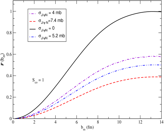
Refer to caption

Figure 1: The centrality dependence of the suppression factor.

In fig.Β (2) we show the centrality dependence of the total $J/\psi$ production cross-section in nucleus-nucleus collisions. It is seen that the survival probability is very sensitive to the choice of $\sigma_{J/\psi N}$ cross-section as well as to the comoving scenario adopted.

Refer to caption

Figure 2: Total $J/\psi$ cross-section in different comoving scenarios (see text) as function of centrality at LHC energies.

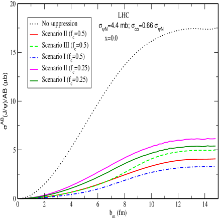
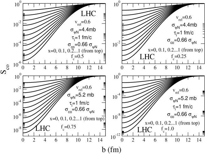
In the second scenario of comoving absorption the survival probability becomes function of $b$ only. So in fig.Β (3) we plot $S_{\mathrm{c}o}$ as a function of impact parameter. The suppression depends on two factors: (i) what fraction ($x$) of produced hadrons come from hard processes and (ii) what fraction ($f_{c}$) of these hadrons (co)move with the $J/\psi$. To show the sensitivity on these two factors we have chosen various combinations of $x$ and $f_{c}$. It is seen that for a given $f_{c}$ as $x$ increases (which is possible as the beam energy increases) the survival probability goes down.

Refer to caption

Figure 3: Comoving survival probability in the scenario II as a function of impact parameter.

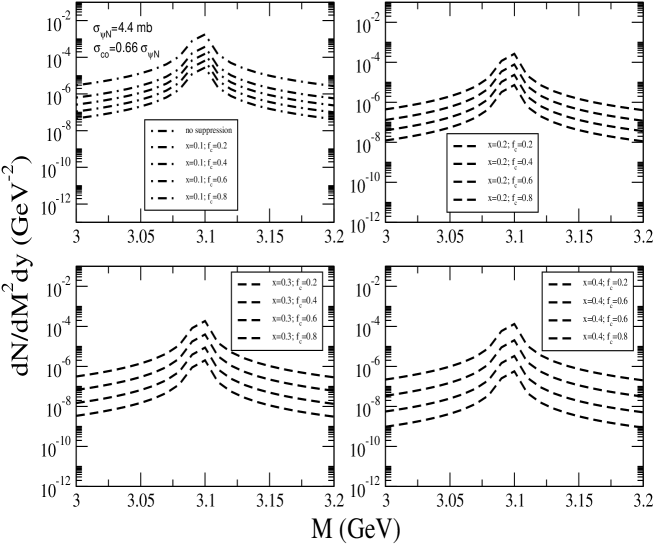
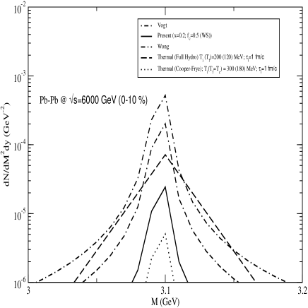
Now let us turn to the lepton pair yield from $J/\psi$ decay. In fig.Β (4) we compare the lepton pair yield from $Pb-Pb$ collisions at $\sqrt{s}=6000$ GeV for 0 - 10 % centrality. We have chosen different combinations of $x$ and $f_{c}$ to show the sensitivity of the results in second scenario of comoving suppression. However, we have checked that for very small values of $x$ and $f_{c}$ the three scenarios for comoving suppression coincide. But for higher value of both $x$ and $f_{c}$ these are quite different. Past (SPS) and present (RHIC) experiments suggest that the value of $x$ may not be very high even at LHC energies. To see the effects of $x$ and $f_{c}$ on the dilepton yield we show in fig.Β (4) the invariant mass distribution for various combinations of these two parameters in the invariant mass range 3 GeV$\,\leq M\,\leq\,$ 3.2 GeV. We notice that for the combination in which both $x$ and $f_{c}$ are large, the yield is less, indicating more suppression as the beam energy increases (since in that case $x$ will be different from zero).

Refer to caption

Figure 4: Dilepton yield in $Pb-Pb$ collisions at $\sqrt{s}=$ 6000 GeV, for various combinations of ($x,f_{c}$) in the second case of comoving absorption.

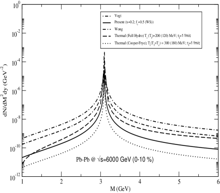
Now we compare the hard contribution with the thermal one in fig.Β (5). For the thermal part we use simple Bjorken cooling law. We assume a hadronic matter initial state with initial temperature of the order of 300 MeV at proper time $\tau_{i}$ = 1 fm. We realise that at $T$ = 300 MeV the hadronic matter the hadronic matter may dissolve to QGP, however, we take such a high temperature to show that the hard contribution is larger than the thermal even for such a large initial temperature. For the hard production we choose a centrality cut of 10 %. For nuclear shadowing EKSΒ [9] parametrization has been used together with CTEQ PDFΒ [6]. We have included a $K$ factor $\sim$ 2.5 to account for higher order processes.

Refer to caption

Figure 5: Dilepton yield in $Pb-Pb$ collisions at $\sqrt{s}=$ 6000 GeV, $x=0.2$ and $f_{c}=0.5$ in different comoving scenarios . Thermal contributions are also included.

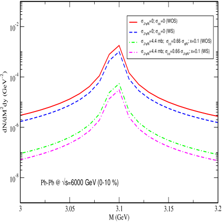
As the beam energy increases the shadowing effect in hard scattering processes becomes important. We have checked that at RHIC energies the lepton pair yields with and without shadowing are not very different. However, there is a substantial difference in the yields at LHC energies (see fig.Β (6)).

Refer to caption

Figure 6: Dilepton yield in $Pb-Pb$ collisions at $\sqrt{s}=$ 6000 GeV, with (WS) and without (WOS) shadowing for two values of absorption cross-sections.

The effects of different comoving scenarios on the dilepton yield is clearly seen in fig.Β (7) in the invariant mass window 3 GeV$\,\leq\,M\,\leq\,$3.2 GeV. We see that the second scenario of the comoving absorption gives the maximum suppression for the given set of parameters. Even, the thermal contribution is larger than the hard contribution. The yield of lepton pairs (hard part) from the experiment at LHC energies might lie between these yields.

Refer to caption

Figure 7: Same as fig.Β (5) with 3 GeV$\,\leq\,M\,\leq\,$3.2 GeV.

IV. Summary and discussions

In this work we have calculated the lepton pairs yield from thermal and hard $J/\psi$ decays. The effects of the various comover scenarios on the survival probability of the heavy quarkonia, nuclear shadowing on the production cross sections of the heavy quarks and the centrality of the collisions have been considered. The effects of shadowing and comover suppressions on the dilepton spectra resulting from the decays of $J/\psi$ is found to be large. The dilepton yield from the thermal $J/\psi$ is found to be smaller than the contributions from hard $J/\psi$.

The fraction of the comover is treated as a parameter here and the lepton pair yields from the heavy quarkonia have been evaluated for various values of this parameter. The increase of $J/\psi$ yield from the decays of higher charmonium states have been neglected here, however the yield with the inclusion of such processes may be realized within the parameters ($x$, the fraction of hard component and $f_{c}$, the fraction of the comoving hadrons) range considered here.

Acknowledgment: One of us (P.R) is grateful to Theory Division, CERN PH-TH for hospitality where part of this work was performed.

References

  • [1] H. Satz and T. Matsui, Phys. Lett. B 178 416 (1986).
  • [2] Dimuon Forward Spectrometer, ALICE Technical Design Report, CERN/LHCC 99-22, August 1999.
  • [3] J. F. Amundson, O. J. P. Eboli, E. M. Gregores, and F. Halzen, Phys. Lett. B390 323 (1997).
  • [4] M. B. Gay Ducati, V. P. Goncalves, and C. B. Mariotto, Phys. Rev. D65 037503 (2002).
  • [5] R. Vogt, Phys. Rep. 310 197 (1999).
  • [6] H. L. Lai et al., Eur. Phys. J. C12 375 (2000); M. Gluck, E. Reya, and A. Vogt, Euro. Phys. J. C5, 461 (1998); A. D. Martin, R. G. Roberts, W. J. Sterling, and R. S. Thorne, Euro. Phys. J. C4, 463 (1998).
  • [7] R. J. Glauber, in Lectures in Theoretical Physics, ed. W. E. Britten and L. G. Dunham, Interscience, N. Y. (1959).
  • [8] C. Y. Wong, Introduction to high energy heavy ion collisions, World Scientific, Singapore (1994).
  • [9] K. J. Eskola, V. J. Kolhinen, and C. A. Salgado, Eur. Phys. J C9 61 (1999).
  • [10] J. D. Bjorken, Phys. Rev. D27 140 (1983).
  • [11] S. Gavin and R. Vogt, Nucl. Phys. B345 104 (1990).
  • [12] R. S. Azevedo and M. Nielson, nucl-th/0407080; Z. Lin and B. Zhang, Phys. Rev. C61 024904 (2000)
  • [13] D. Kharzeev and M. Nardi, Phys. Lett. B507 121 2001.
  • [14] F. Cooper and G. Frye, Phys. Rev. D 10, (1974) 186.