Single-Particle Properties from Kohn–Sham Green’s Functions

Abstract

An effective action approach to Kohn–Sham density functional theory is used to illustrate how the exact Green’s function can be calculated in terms of the Kohn–Sham Green’s function. An example based on Skyrme energy functionals shows that single-particle Kohn–Sham spectra can be improved by adding sources used to construct the energy functional.

The Skyrme-Hartree–Fock approach to nuclear properties has had wide success in reproducing bulk properties of nuclei across the periodic table VB72 ; RINGSCHUCK ; BROWN98 ; Dobaczewski:2001ed ; BENDER2003 ; Stoitsov:2003pd . The interpretation of the Skyrme formalism as an approximate implementation of Kohn–Sham density functional theory (DFT) BRACK85 implies that certain observables (energy per particle, densities) can be calculated reliably, but these do not include single-particle quantities. Only for the bulk observables can the DFT framework accommodate all correlations in principle (if not in practice because of the limited form of the energy functionals actually used) KOHN65 ; PARR89 ; DREIZLER90 . Nevertheless, single-particle energies and wave functions from Skyrme and other DFT-like formalisms are also regularly used.

In this letter, we illustrate how to extend the effective action approach to Kohn–Sham DFT VALIEV96 ; RASAMNY98 ; PUG02 ; FURNSTAHL04b to calculate the full single-particle Green’s function in terms of Kohn–Sham Green’s functions at the same level of approximation. Our discussion directly adapts the extension described in the context of Coulomb systems in Refs. VALIEV97 ; VALIEV97b . This connection between Green’s functions helps to clarify both some misconceptions and limitations of the Kohn–Sham approach, and suggests how to improve calculations of single-particle properties. At first, we consider functionals of the fermion density only, and then compare to generalized functionals that also depend on the kinetic energy density to illustrate the effect of additional sources.

We introduce a generating functional in the path integral formulation with a Lagrangian ${\cal L}$ supplemented by a local c-number source $J(x)$ coupled to the composite density operator as in Ref. PUG02 , but add a non-local c-number source $\xi(x,x^{\prime})_{\alpha\beta}$ coupled to $\psi_{\alpha}(x)\psi_{\beta}^{\dagger}(x^{\prime})$,

$$Z[J,\xi]=e^{iW[J,\xi]}=\int\!D\psi D\psi^{\dagger}\ e^{i\int\!d^{4}x\ [{\cal L}\,+\,J(x)\psi_{\alpha}^{\dagger}(x)\psi_{\alpha}(x)\,+\,\int\!d^{4}x^{\prime}\,\psi_{\alpha}(x)\xi(x,x^{\prime})_{\alpha\beta}\psi_{\beta}^{\dagger}(x^{\prime})]}\ ,$$ (1)

where $\alpha$ and $\beta$ are spin indices and summation of repeated indices is implied. (We generalize below to an additional local source, as in Ref. FURNSTAHL04b .) For simplicity, normalization factors are considered to be implicit in the functional integration measure FUKUDA94 ; FUKUDA95 . As a specific example, we will use the effective field theory (EFT) Lagrangian appropriate for a dilute Fermi system HAMMER00 , but the discussion can be adapted to any system for which a hierarchy of approximations can be defined.

The fermion density in the presence of the sources $J$ and $\xi$ is

$$\rho(x)\equiv\langle\psi_{\alpha}^{\dagger}(x)\psi_{\alpha}(x)\rangle_{J\,,\,\xi}=\frac{1}{iZ}\frac{\delta Z[J,\xi]}{\delta J(x)}=\frac{\delta W[J,\xi]}{\delta J(x)}\ .$$ (2)

Note that the sources here are time dependent, in contrast to the more limited discussion with static sources in Ref. PUG02 ; however, the generalization of the formalism is direct. A functional Legendre transformation from $J$ to $\rho$, which takes us from $W$ to the effective action $\Gamma$, produces an energy functional of the density, which is minimized at the exact ground-state density for time-independent sources. The inversion method FUKUDA94 ; FUKUDA95 carries out this inversion order-by-order in a specified expansion; an EFT expansion was used in Refs. PUG02 and FURNSTAHL04b . At the end, one sets $J(x)$ and $\xi(x,x^{\prime})$ to zero. (Although we are unaware of any general problems, we have not excluded the possibility of complications in making the inversions with time-dependent sources.)

Solving the zeroth-order system defines the Green’s function ${G}_{{\rm ks}}(x,x^{\prime})_{\alpha\beta}$ of the Kohn–Sham non-interacting system in the presence of $\xi(x,x^{\prime})_{\alpha\beta}$, the Kohn–Sham potential $J_{0}(x)$, and an external potential $v({\bf x})$. This Green’s function satisfies

$$\int\!d^{4}z\ [{G}_{{\rm ks}}(x,z)]_{\alpha\gamma}^{-1}{G}_{{\rm ks}}(z,x^{\prime})_{\gamma\beta}=\delta_{\alpha\beta}\delta^{4}(x-x^{\prime})\ ,$$ (3)

or

$$\int\!d^{4}z\left[\left(i\partial_{t}+\frac{\bm{\nabla}^{2}}{2M}-v({\bf\bf{x}})+J_{0}(x)\right)\delta_{\alpha\gamma}\delta^{4}(x-z)-\xi(z,x)_{\gamma\alpha}\right]{G}_{{\rm ks}}(z,x^{\prime})_{\gamma\beta}=\delta_{\alpha\beta}\delta^{4}(x-x^{\prime})\ ,$$ (4)

with appropriate finite-density boundary conditions (one could also introduce a chemical potential). Note that ${G}_{{\rm ks}}$ doesn’t take a simple form in terms of orbitals [see ${G}_{{\rm ks}}^{0}$ in Eq. (21)] until we set $\xi=0$ and restrict ourselves to time independent $J_{0}$.

Functional derivatives of $W$ with respect to $\xi(x,x^{\prime})$ gives the two-point function in the presence of the sources,

$$iG(x,x^{\prime})_{\alpha\beta}\equiv\langle T[\psi_{\alpha}(x)\psi_{\beta}^{\dagger}(x^{\prime})]\rangle_{J,\xi}=\frac{1}{iZ}\frac{\delta Z[J,\xi]}{\delta\xi(x,x^{\prime})_{\alpha\beta}}=\frac{\delta W[J,\xi]}{\delta\xi(x,x^{\prime})_{\alpha\beta}}\ .$$ (5)

The exact ground-state Green’s function is obtained by setting $\xi=J=0$ after taking derivatives. The key results we will need to evaluate Eq. (5) in terms of Kohn–Sham quantities were given in Refs. VALIEV97 ; VALIEV97b (we follow their notation for the most part) and are rederived here. First, functional derivatives with respect to $\xi$ of $W$ and $\Gamma$ are directly related, where

$$\Gamma[\rho,\xi]=W[J,\xi]-\int\!d^{4}y\,J(y)\rho(y)$$ (6)

is the effective action. Namely, the functional derivative with respect to $\xi$ of this equation yields (spin indices are suppressed)

$$\left(\frac{\delta\Gamma[\rho,\xi]}{\delta\xi(x,x^{\prime})}\right)_{\rho}=\left(\frac{\delta W[J,\xi]}{\delta\xi(x,x^{\prime})}\right)_{J}+\int\!d^{4}y\left(\frac{\delta W[J,\xi]}{\delta J(y)}\right)_{\xi}\left(\frac{\delta J(y)}{\delta\xi(x,x^{\prime})}\right)_{\rho}-\int\!d^{4}y\left(\frac{\delta J(y)}{\delta\xi(x,x^{\prime})}\right)_{\rho}\,\rho(y)\ ,$$ (7)

from which the last two terms cancel, leaving

$$\left(\frac{\delta W[J,\xi]}{\delta\xi(x,x^{\prime})_{\alpha\beta}}\right)_{J}=\left(\frac{\delta\Gamma[\rho,\xi]}{\delta\xi(x,x^{\prime})_{\alpha\beta}}\right)_{\rho}\ .$$ (8)

(Here and below we repeatedly apply the functional relations

$$\left(\frac{\delta F}{\delta\xi}\right)_{\rho}=\left(\frac{\delta F}{\delta\xi}\right)_{J}+\left(\frac{\delta F}{\delta J}\right)_{\xi}\left(\frac{\delta J}{\delta\xi}\right)_{\rho}=\left(\frac{\delta F}{\delta\xi}\right)_{J}-\left(\frac{\delta F}{\delta\rho}\right)_{\xi}\left(\frac{\delta\rho}{\delta\xi}\right)_{J}\ ,$$ (9)

where $F=F[J,\xi]$ and arguments and integrals are implied.) Equation (8) is a special case of a general result for Legendre transformations proved in Ref. ZINNJUSTIN .

Next, this relation applied to the zeroth-order (Kohn–Sham) system yields the Kohn–Sham Green’s function,

$$\left(\frac{\delta\Gamma_{0}[\rho,\xi]}{\delta\xi(x,x^{\prime})_{\alpha\beta}}\right)_{\rho}=\left(\frac{\delta W_{0}[J_{0},\xi]}{\delta\xi(x,x^{\prime})_{\alpha\beta}}\right)_{J_{0}}=i{G}_{{\rm ks}}(x,x^{\prime})_{\alpha\beta}\ .$$ (10)

We divide the full effective action into zeroth-order and interacting pieces,

$$\Gamma[\rho,\xi]=\Gamma_{0}[\rho,\xi]+\Gamma_{\rm int}[\rho,\xi]\ .$$ (11)

Since $\Gamma_{\rm int}[\rho,\xi]$ depends on $\xi$ only through ${G}_{{\rm ks}}$,

$$\left(\frac{\delta\Gamma_{\rm int}[\rho,\xi]}{\delta\xi(x,x^{\prime})_{\alpha\beta}}\right)_{\rho}=\int\!\!\int\!\frac{\delta\Gamma_{\rm int}[\rho,\xi]}{\delta{G}_{{\rm ks}}(y,y^{\prime})_{\delta\gamma}}\,\left(\frac{\delta{G}_{{\rm ks}}(y,y^{\prime})_{\delta\gamma}}{\delta\xi(x,x^{\prime})_{\alpha\beta}}\right)_{\rho}\ dy\,dy^{\prime}\ .$$ (12)

The second half of the integrand can be rewritten

$$\left(\frac{\delta{G}_{{\rm ks}}(y,y^{\prime})_{\delta\gamma}}{\delta\xi(x,x^{\prime})_{\alpha\beta}}\right)_{\rho} = \left(\frac{\delta{G}_{{\rm ks}}(y,y^{\prime})_{\delta\gamma}}{\delta\xi(x,x^{\prime})_{\alpha\beta}}\right)_{J_{0}}+\int\!\left(\frac{\delta{G}_{{\rm ks}}(y,y^{\prime})_{\delta\gamma}}{\delta J_{0}(z)}\right)_{\xi}\left(\frac{\delta J_{0}(z)}{\delta\xi(x,x^{\prime})_{\alpha\beta}}\right)_{\rho}\,dz$$ (13)

$$= \left(\frac{\delta{G}_{{\rm ks}}(y,y^{\prime})_{\delta\gamma}}{\delta\xi(x,x^{\prime})_{\alpha\beta}}\right)_{J_{0}}-\int\!\left(\frac{\delta{G}_{{\rm ks}}(y,y^{\prime})_{\delta\gamma}}{\delta\rho(z)}\right)_{\xi}\left(\frac{\delta\rho(z)}{\delta\xi(x,x^{\prime})_{\alpha\beta}}\right)_{J_{0}}\,dz$$

$$= {G}_{{\rm ks}}(x,y^{\prime})_{\alpha\gamma}{G}_{{\rm ks}}(y,x^{\prime})_{\delta\beta}$$

$$\qquad\hbox{}+i\int\!\left(\frac{\delta{G}_{{\rm ks}}(y,y^{\prime})_{\delta\gamma}}{\delta\rho(z)}\right)_{\xi}{G}_{{\rm ks}}(x,z)_{\alpha\lambda}{G}_{{\rm ks}}(z,x^{\prime})_{\lambda\beta}\,dz\ .$$

The second line follows by applying Eq. (9) with $F\rightarrow{G}_{{\rm ks}}$ and simplifying. The functional derivatives in the second line can be evaluated by using the expression for ${G}_{{\rm ks}}$ in terms of the noninteracting generating functionals. Thus,

$$\left(\frac{\delta{G}_{{\rm ks}}(y,y^{\prime})_{\delta\gamma}}{\delta\xi(x,x^{\prime})_{\alpha\beta}}\right)_{J_{0}} = \frac{\delta}{\delta\xi(x,x^{\prime})_{\alpha\beta}}\left[-\frac{1}{Z_{0}}\frac{\delta Z_{0}[J_{0},\xi]}{\delta\xi(y,y^{\prime})_{\delta\gamma}}\right]$$ (14)

$$= \left[\frac{1}{Z_{0}}\frac{\delta Z_{0}[J_{0},\xi]}{\delta\xi(x,x^{\prime})_{\alpha\beta}}\right]\left[\frac{1}{Z_{0}}\frac{\delta Z_{0}[J_{0},\xi]}{\delta\xi(y,y^{\prime})_{\delta\gamma}}\right]-\frac{1}{Z_{0}}\frac{\delta^{2}Z_{0}[J_{0},\xi]}{\delta\xi(x,x^{\prime})_{\alpha\beta}\,\delta\xi(y,y^{\prime})_{\delta\gamma}}$$

$$= i^{2}\langle T[\psi_{\alpha}(x)\psi^{\dagger}_{\beta}(x^{\prime})]\rangle\,\langle T[\psi_{\delta}(y)\psi^{\dagger}_{\gamma}(y^{\prime})]\rangle-i^{2}\langle T[\psi_{\alpha}(x)\psi^{\dagger}_{\beta}(x^{\prime})\psi_{\delta}(y)\psi^{\dagger}_{\gamma}(y^{\prime})]\rangle$$

$$= (-i)^{2}\langle T[\psi_{\alpha}(x)\psi^{\dagger}_{\gamma}(y^{\prime})]\rangle\,\langle T[\psi_{\delta}(y)\psi^{\dagger}_{\beta}(x^{\prime})]\rangle$$

$$= {G}_{{\rm ks}}(x,y^{\prime})_{\alpha\gamma}\,{G}_{{\rm ks}}(y,x^{\prime})_{\delta\beta}\ ,$$

where we’ve applied Wick’s theorem to the noninteracting system to go from the third line to the fourth line, and

$$\left(\frac{\delta\rho(z)}{\delta\xi(x,x^{\prime})_{\alpha\beta}}\right)_{J_{0}}=-i\left(\frac{\delta{G}_{{\rm ks}}(z,z^{+})_{\delta\delta}}{\delta\xi(x,x^{\prime})_{\alpha\beta}}\right)_{J_{0}}=-i{G}_{{\rm ks}}(x,z)_{\alpha\delta}\,{G}_{{\rm ks}}(z,x^{\prime})_{\delta\beta}\ .$$ (15)

Alternatively, we can expand $\delta({G}_{{\rm ks}}{G}_{{\rm ks}}^{-1})/\delta\xi=0$ and use $\delta{G}_{{\rm ks}}^{-1}/\delta\xi=-1$.

Substituting Eq. (13) back into Eq. (12), we find that

$$\left(\frac{\delta\Gamma_{\rm int}[\rho,\xi]}{\delta\xi(x,x^{\prime})_{\alpha\beta}}\right)_{\rho} = \int\!\!\int\!{G}_{{\rm ks}}(x,y^{\prime})_{\alpha\gamma}\,\frac{\delta\Gamma_{\rm int}[\rho,\xi]}{\delta{G}_{{\rm ks}}(y,y^{\prime})_{\delta\gamma}}\,{G}_{{\rm ks}}(y,x^{\prime})_{\delta\beta}\ dy\,dy^{\prime}$$ (16)

$$\hbox{}+i\int\!{G}_{{\rm ks}}(x,y)_{\alpha\lambda}\left(\frac{\delta\Gamma_{\rm int}[\rho,\xi]}{\delta\rho(y)}\right)_{\xi}{G}_{{\rm ks}}(y,x^{\prime})_{\lambda\beta}\ dy\ .$$

Equations (10) and (16), together with

$$iG(x,x^{\prime})_{\alpha\beta}=\left(\frac{\delta W[J,\xi]}{\delta\xi(x,x^{\prime})_{\alpha\beta}}\right)_{J}=\left(\frac{\delta\Gamma[\rho,\xi]}{\delta\xi(x,x^{\prime})_{\alpha\beta}}\right)_{\rho}=\left(\frac{\delta\Gamma_{0}[\rho,\xi]}{\delta\xi(x,x^{\prime})_{\alpha\beta}}\right)_{\rho}+\left(\frac{\delta\Gamma_{\rm int}[\rho,\xi]}{\delta\xi(x,x^{\prime})_{\alpha\beta}}\right)_{\rho}\ ,$$ (17)

imply a Dyson equation for the exact Green’s function:

$$G(x,x^{\prime})_{\alpha\beta}={G}_{{\rm ks}}(x,x^{\prime})_{\alpha\beta}+\int\!{G}_{{\rm ks}}(x,y^{\prime})_{\alpha\gamma}\,\Sigma_{\rm ks}(y^{\prime},y)_{\gamma\delta}\,{G}_{{\rm ks}}(y,x^{\prime})_{\delta\beta}\ dy\,dy^{\prime}\ ,$$ (18)

which defines a self-energy $\Sigma_{\rm ks}$ as

$$\Sigma_{\rm ks}(y^{\prime},y)_{\gamma\delta} = \frac{1}{i}\frac{\delta\Gamma_{\rm int}[\rho,\xi]}{\delta{G}_{{\rm ks}}(y,y^{\prime})_{\delta\gamma}}\,+\left(\frac{\delta\Gamma_{\rm int}[\rho,\xi]}{\delta\rho(y)}\right)_{\xi}\delta_{\gamma\delta}\,\delta^{4}(y^{\prime}-y)$$ (19)

$$\equiv \Sigma^{\prime}_{\rm ks}(y^{\prime},y)_{\gamma\delta}+J_{0}(y^{\prime})\,\delta_{\gamma\delta}\,\delta^{4}(y^{\prime}-y)\ .$$

In the second line, the self-consistent Kohn–Sham potential $J_{0}$ is equal to $\delta\Gamma_{\rm int}/\delta\rho$ only when we set $J=0$ PUG02 . Neither $\Sigma_{\rm ks}$ nor $\Sigma^{\prime}_{\rm ks}$ is the conventional self-energy, which is built from non-interacting (rather than Kohn–Sham) Green’s functions. We can obtain $\Sigma^{\prime}_{\rm ks}(y^{\prime},y)$ at the diagrammatic level by opening each ${G}_{{\rm ks}}$ line in turn in a given Feynman diagram for $\Gamma_{\rm int}$. It consists of the same diagrams as the conventional one-particle-reducible self-energy, but with the fermion lines given by ${G}_{{\rm ks}}$ rather than the non-interacting Green’s function (which includes only the external potential).

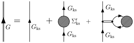
Figure 1: Equation for the full propagator in terms of the Kohn–Sham Green’s functions and self-energy.

Now consider applying these equations with $\xi=J=0$ after taking functional derivatives; we denote the Kohn–Sham Green’s function in this case as ${G}_{{\rm ks}}^{0}$. For simplicity we will consider spin-independent interactions, so that the Green’s functions and self-energies are diagonal in spin. Kohn–Sham orbitals arise as solutions to

$$\bigl{[}-\frac{\bm{\nabla}^{2}}{2M}+v({\bf\bf{x}})-J_{0}({\bf\bf{x}})\bigr{]}\,\psi_{k}({\bf x})=\varepsilon_{k}\psi_{k}({\bf x})\,,$$ (20)

where the index $k$ represents all quantum numbers except for the spin PUG02 . The decomposition of ${G}_{{\rm ks}}^{0}(x,x^{\prime})_{\alpha\beta}=\delta_{\alpha\beta}{G}_{{\rm ks}}^{0}(x,x^{\prime})$ in terms of these orbitals is PUG02

$$i{G}_{{\rm ks}}^{0}({\bf\bf{x}}t,{\bf\bf{x}}^{\prime}t^{\prime})=\sum_{k}\psi_{k}({\bf\bf{x}})\,\psi_{k}^{*}({\bf\bf{x}}^{\prime})\,e^{-i\varepsilon_{k}(t-t^{\prime})}[\theta(t-t^{\prime})\,\theta(\varepsilon_{k}-\varepsilon_{\rm F})-\theta(t^{\prime}-t)\,\theta(\varepsilon_{\rm F}-\varepsilon_{k})]\ ,$$ (21)

corresponding (in frequency space) to simple poles, just like a Hartree Green’s function. It is well known that the Kohn–Sham single-particle eigenvalues $\varepsilon_{k}$ are not physical except at the Fermi surface PARR89 ; DREIZLER90 . Nevertheless, the trace of this Green’s function gives the complete ground-state density $\rho({\bf\bf{x}})$ (that is, the exact result if we calculate to all orders).

We can easily show diagrammatically that Eq. (18) implies that the density obtained from the Kohn–Sham Green’s function is, as advertised, exactly equal to that obtained from the exact Green’s function. The density can be directly expressed in terms of the Kohn–Sham Green’s function with equal arguments as

$$\rho({\bf\bf{x}})=-i\,{G}_{{\rm ks}}^{0}(x,x^{+})_{\alpha\alpha}=-i\nu\,{G}_{{\rm ks}}^{0}(x,x^{+})\ ,$$ (22)

where $\nu$ is the spin-isospin degeneracy. In Fig. 1, we have rewritten the last term in the Dyson equation (18) for the exact Green’s function using

$$\frac{\delta\Gamma_{\rm int}}{\delta\rho({\bf y})}=\int\!\frac{\delta\Gamma_{\rm int}}{\delta J_{0}({\bf z})}\frac{\delta J_{0}({\bf z})}{\delta\rho({\bf y})}\ d^{3}{\bf z}\ ,$$ (23)

where $\delta J_{0}({\bf z})/\delta\rho({\bf y})=[\delta^{2}W_{0}/\delta J_{0}({\bf y})\delta J_{0}({\bf z})]^{-1}$, which is minus the inverse density-density correlator VALIEV97 ; PUG02 , is represented with a double line (with no arrow). The result of carrying out Eq. (22) on Eq. (18) is shown in Fig. 2, where the last two diagrams cancel as in Fig. 3. Note that while similar cancellations were shown in Ref. PUG02 in the special case of zero-range interactions, the result here is completely general. Thus we see that the exact density is reproduced by the Kohn–Sham Green’s function by construction.

Figure 2: Equation for the density, showing the equivalence of the full and Kohn–Sham densities.

Figure 3: Cancellation of the density-density correlator with $\delta J_{0}/\delta\rho$.

To illustrate some issues in comparing Kohn–Sham and exact Green’s functions, we apply the formalism with the effective Lagrangian for dilute Fermi systems used in prior investigations:

$${\cal L} = \psi^{\dagger}\biggl{[}i\partial_{t}+\frac{\overrightarrow{\nabla}^{\,2}}{2M}\biggr{]}\psi-\frac{C_{0}}{2}(\psi^{\dagger}\psi)^{2}+\frac{C_{2}}{16}\Bigl{[}(\psi\psi)^{\dagger}(\psi\tensor{\nabla}^{2}\psi)+\mbox{ h.c.}\Bigr{]}$$ (24)

$$\hbox{}+\frac{C_{2}^{\prime}}{8}(\psi\tensor{\nabla}\psi)^{\dagger}\cdot(\psi\tensor{\nabla}\psi)+\cdots\ ,$$

where $\tensor{\nabla}=\overleftarrow{\nabla}-\overrightarrow{\nabla}$ is the Galilean invariant derivative and h.c. denotes the Hermitian conjugate. To describe trapped fermions, we add to the Lagrangian a term for an external confining potential $v({\bf\bf{x}})$ coupled to the density operator $v({\bf\bf{x}})\psi^{\dagger}\psi$ PUG02 . For the numerical calculations, we take the potential to be an isotropic harmonic confining potential,

$$v({\bf\bf{x}})=\frac{1}{2}m\,\omega^{2}\,|{\bf\bf{x}}|^{2}\ ,$$ (25)

although the discussion holds for a general non-vanishing external potential.

We repeat the previous development to introduce a second energy functional with an additional local source coupled to the kinetic energy density, following Ref. FURNSTAHL04b . The comparison of results from the two functionals illustrates how the Kohn–Sham single-particle spectrum can be significantly different even though the bulk observables are essentially equal FURNSTAHL04b . So we consider

$$Z^{\prime}[J,\eta,\xi]=e^{iW^{\prime}[J,\eta,\xi]}=\int\!D\psi D\psi^{\dagger}\ e^{i\int\!d^{4}x\ [{\cal L}\,+\,J\psi^{\dagger}\psi\,+\,\eta\bm{\nabla}\psi^{\dagger}\cdot\bm{\nabla}\psi\,+\,\int\!d^{4}x^{\prime}\,\psi(x)\xi(x,x^{\prime})\psi^{\dagger}(x^{\prime})]}\ ,$$ (26)

and the corresponding effective action

$$\Gamma^{\prime}[\rho,\tau,\xi]=W^{\prime}[J,\eta,\xi]-\int\!d^{4}y\,J(y)\rho(y)-\int\!d^{4}y\ \eta(y)\tau(y)\ ,$$ (27)

with kinetic energy density

$$\tau(x)\equiv\langle\bm{\nabla}\psi^{\dagger}(x)\bm{\cdot\nabla}\psi(x)\rangle_{J\,,\,\eta\,,\,\xi}=\frac{\delta W^{\prime}[J,\eta,\xi]}{\delta\eta(x)}\ .$$ (28)

(We use superscript primes on the functionals, and $\mbox{ks}^{\prime}$ on the self-energies and Green’s functions to distinguish the following quantities from those without $\eta$ or $\tau$ dependence.) Each step goes through with straightforward generalizations, yielding Eq. (18) again, but now with

$$\Sigma_{\rm ks^{\prime}}(y^{\prime},y)_{\gamma\delta} = \frac{\delta\Gamma^{\prime}_{\rm int}[\rho,\tau,\xi]}{\delta{G}_{{\rm ks}^{\prime}}(y,y^{\prime})_{\delta\gamma}}\,+[J_{0}(y^{\prime})+\bm{\nabla}_{y^{\prime}}\bm{\cdot}\bm{\nabla}_{y}\,\eta_{0}(y^{\prime})]\,\delta_{\gamma\delta}\,\delta^{4}(y^{\prime}-y)$$ (29)

$$\equiv \Sigma^{\prime}_{\rm ks^{\prime}}(y^{\prime},y)_{\gamma\delta}+[J_{0}(y^{\prime})+\bm{\nabla}_{y^{\prime}}\bm{\cdot}\bm{\nabla}_{y}\,\eta_{0}(y^{\prime})]\,\delta_{\gamma\delta}\,\delta^{4}(y^{\prime}-y)$$

after $J(y^{\prime})$ and $\eta(y^{\prime})$ are set to zero. [Note that the gradients act on the ${G}_{{\rm ks}^{\prime}}$’s to produce $\tau$ after partial integrations in Eq. (18).]

These two functionals were compared in Ref. FURNSTAHL04b for a dilute gas of fermions in a harmonic trap. Two sets of parameters were used to illustrate the impact of a larger effective mass $M^{*}({\bf\bf{x}})$, which appears only in the “$\rho\tau$” (primed) formalism. Even though the fermion density and energy per particle for the $\rho$ and $\rho\tau$ functionals were very similar, the single-particle spectra have significant and systematic differences (see Ref. FURNSTAHL04b for details and figures). We can understand the systematics of the difference by comparing Kohn–Sham and exact spectra for a uniform system. We will drop the non-Hartree–Fock terms, which have been treated in LDA in both cases and which contribute equally to the energy spectra. We note that the terms in the $\rho\tau$ functional correspond directly with terms in conventional Skyrme energy functionals FURNSTAHL04b .

In the $\rho$ case, the Kohn–Sham equation for the single-particle orbital PUG02 (with external potential set to zero) leads to the spectrum

$$\varepsilon_{k}^{\rho}=\frac{k^{2}}{2M}-J^{\rho}_{0}\ ,$$ (30)

where

$$J_{0}^{\rho}=-\frac{\nu-1}{\nu}\,C_{0}\rho-\left((\nu-1)\frac{C_{2}}{15\pi^{2}}+(\nu+1)\frac{C^{\prime}_{2}}{15\pi^{2}}\right)\left(\frac{6\pi^{2}\rho}{\nu}\right)^{5/3}\ .$$ (31)

In the $\rho\tau$ case, we find a different spectrum

$$\varepsilon_{k}^{\rho\tau}=\frac{k^{2}}{2M^{*}}-J^{\rho\tau}_{0}\ ,$$ (32)

where

$$J_{0}^{\rho\tau}=-\frac{\nu-1}{\nu}\,C_{0}\rho-\left(\frac{\nu-1}{\nu}\,\frac{C_{2}}{4}+\frac{\nu+1}{\nu}\,\frac{C^{\prime}_{2}}{4}\right)\tau\ ,$$ (33)

and

$$\frac{1}{2M^{*}}=\frac{1}{2M}-{\eta_{0}}=\frac{1}{2M}+\left(\frac{\nu-1}{\nu}\,\frac{C_{2}}{4}+\frac{\nu+1}{\nu}\,\frac{C^{\prime}_{2}}{4}\right)\rho\ .$$ (34)

Using $\tau=\frac{3}{5}k_{\rm F}^{2}\rho$, the difference in the spectra simplifies to

$$\varepsilon^{\rho}_{k}-\varepsilon^{\rho\tau}_{k}=\left(\frac{\nu-1}{\nu}\,\frac{C_{2}}{4}+\frac{\nu+1}{\nu}\,\frac{C^{\prime}_{2}}{4}\right)(k_{\rm F}^{2}-k^{2})\rho\ .$$ (35)

Thus, the spectra differ for all momentum states except at the Fermi surface, where the spectra coincide as expected in Kohn–Sham DFT. In detail, the $\rho\tau$ spectrum includes explicit momentum dependence that is converted to density dependence (i.e., $k_{\rm F}$ dependence) in the $\rho$ spectrum. We can also compare the Kohn-Sham spectra to that of the Green’s function in the Hartree–Fock approximation, where we find that the $\varepsilon^{\rho\tau}$ spectrum is the same as the Hartree–Fock spectrum. Indeed, for this approximation the $J_{0}$ and $\eta_{0}$ terms in Eq. (29) precisely cancel against $\Sigma^{\prime}_{\rm ks^{\prime}}$. In contrast, Eq. (19) yields a net contribution that shifts the Kohn–Sham spectrum to the Hartree–Fock spectrum.

This example illustrates how individual Hartree–Fock self-energies in a gradient expansion can be completely included by adding the corresponding source terms. (A different example with covariant energy functionals is given in Ref. FURNSTAHL04c .) The exact cancellations are only possible for local self-energies, which means Hartree–Fock. Beyond Hartree–Fock, the single-particle spectrum from the Kohn–Sham and exact Green’s functions will necessarily differ. We can anticipate that self-energies with large non-localities will lead to the most significant differences. This is consistent with the expectation that low-lying vibrational states can account for the difference in level density between Skyrme (or other mean-field) and experimental spectra near the Fermi surface RINGSCHUCK ; BENDER2003 .

In this work, we have illustrated the relationship between Kohn–Sham and exact Green’s functions within an effective action formalism. This approach goes beyond the observation that single-particle properties are not reliably calculated in terms of Kohn–Sham orbitals and eigenvalues. The formalism presents two ways to improve single-particle spectra. The Kohn–Sham spectra became closer to the exact spectra with the addition of appropriate sources. It is tempting to conclude that adding additional sources can always improve the Kohn–Sham single-particle spectrum, but this will require tests beyond the Hartree–Fock level. More generally, Eq. (18) shows how to calculate single-particle quantities in terms of Kohn–Sham propagators at the same level of approximation (which is determined by the truncation of $\Gamma_{\rm int}$). In future work, the formalism will be applied to the calculation of spectral functions and the effect of low-lying vibrational states on the spectra tested by including self-energy diagrams that sum particle-hole bubbles.

References

• (1) D. Vautherin and D. M. Brink, Phys. Rev.  C5 (1972) 626.
• (2) P.  Ring and P.  Gross, The Nuclear Many-Body Problem (Springer-Verlag 2000).
• (3) B. A. Brown, Phys. Rev. C58 (1998) 220, and references therein.
• (4) J. Dobaczewski, W. Nazarewicz and P. G. Reinhard, Nucl. Phys. A 693, 361 (2001) [arXiv:nucl-th/0103001].
• (5) M. Bender, P. H. Heenen, and P.-G. Reinhard, Rev. Mod. Phys. 75 (2003) 121.
• (6) M. V. Stoitsov, J. Dobaczewski, W. Nazarewicz, S. Pittel and D. J. Dean, Phys. Rev. C 68, 054312 (2003), and references therein.
• (7) M. Brack, Helv. Phys. Acta 58 (1985) 715.
• (8) W. Kohn and L. J. Sham, Phys. Rev.  A140 (1965) 1133.
• (9) R. G. Parr and W. Yang, Density Functional Theory of Atoms and Molecules (Oxford University Press, New York, 1989)
• (10) R. M. Dreizler and E. K. U. Gross, Density Functional Theory (Springer, Berlin, 1990).
• (11) M. Valiev and G. W. Fernando, Phys. Rev. B 54 (1996) 7765.
• (12) M. Rasamny, M. M. Valiev, and G. W. Fernando, Phys. Rev. B 58 (1998) 9700.
• (13) A. Bhattacharyya and R. J. Furnstahl, nucl-th/0408014.
• (14) S.J. Puglia, A. Bhattacharyya and R.J. Furnstahl, Nucl. Phys. A723 (2003) 145.
• (15) M. Valiev and G. W. Fernando, arXiv:cond-mat/9702247 (1997), unpublished.
• (16) M. Valiev and G. W. Fernando, Phys. Lett. A 227 (1997) 265.
• (17) R. Fukuda, T. Kotani, Y. Suzuki, and S. Yokojima, Prog. Theor. Phys. 92 (1994) 833.
• (18) R. Fukuda, M. Komachiya, S. Yokojima, Y. Suzuki, K. Okumura, and T. Inagaki, Prog. Theor. Phys. Suppl. 121 (1995) 1.
• (19) H.-W. Hammer and R.J. Furnstahl, Nucl. Phys. A678 (2000) 277.
• (20) J. Zinn-Justin, Quantum Field Theory and Critical Phenomena (Oxford, New York, 2002).
• (21) R. J. Furnstahl and B. D. Serot, in preparation.