Antisymmetrized Green’s function approach to $(e,e^{\prime})$ reactions with a realistic nuclear density

Abstract

A completely antisymmetrized Green’s function approach to the inclusive quasielastic $(e,e^{\prime})$ scattering, including a realistic one-body density, is presented. The single particle Green’s function is expanded in terms of the eigenfunctions of the nonhermitian optical potential. This allows one to treat final state interactions consistently in the inclusive and in the exclusive reactions. Nuclear correlations are included in the one-body density. Numerical results for the response functions of ¹⁶O and ⁴⁰Ca are presented and discussed.

, ,

1 Introduction

The one-body mechanism gives a natural interpretation of the inclusive electron scattering in the quasielastic region. However, in order to explain the experimental data of the separated longitudinal and transverse responses more complicated mechanisms are needed. A review of the experimental data and their possible explanations can be found in Ref. [1]. Thereafter, only a few experimental papers were published [2, 3], while new experiments with high resolution are planned at JLab [4].

Many papers were published in order to explain the problems raised by the separation, i.e., the apparent lack of strength in the longitudinal response and the apparent excess of strength in the transverse one. Among them, the more recent ones are concerned with the contribution to the inclusive cross section of meson exchange currents and isobar excitations [5, 6, 7, 8], with the effect of correlations [9, 10], and the use of a relativistic framework in the calculations [7, 11].

At present, however, a consistent and simultaneous description of the longitudinal and transverse response functions is not available. A possible solution could be the combined effect of two-body currents and tensor correlations [12, 9, 13].

A peculiar problem of inclusive electron scattering is the treatment of final state interactions (FSI), since they are essential to explain the exclusive reaction with one-nucleon emission, which is the dominant process contributing to the inclusive reaction in the quasielastic region. The large absorption due, e.g., to the imaginary part of the optical potential, produces a loss of flux that is appropriate for the exclusive process, but inconsistent for the inclusive one, where the total flux must be conserved. This conservation is preserved in the Green’s function approach considered here. This result was originally derived by arguments based on the multiple scattering theory [14] and then by means of the Feshbach projection operator formalism [15, 16, 17, 18, 11].

The spectral representation of the single-particle (s.p.) Green’s function, based on a biorthogonal expansion in terms of the eigenfunctions of the nonhermitian optical potential, allows one to perform explicit calculations and to treat FSI consistently in the inclusive and in the exclusive reactions. In previous papers [17, 11] the Green’s function approach was used both in a nonrelativistic and in a relativistic framework to perform explicit calculations of the inclusive response functions.

Two issues are the main goal of this paper: a completely antisymmetrized presentation of the Green’s function approach, and the effect of nuclear correlations, which are included in the model through the use of a realistic one-body density matrix (ODM). In the previous application of the method [17, 11] correlations were neglected. The response functions were given by a sum over the residual nucleus states restricted to be s.p. one-hole states in the target. A pure shell model was assumed for the nuclear structure and therefore the overlap functions between the target and the residual nucleus were given by phenomenological s.p. wave functions with a shell-model spectroscopic factor. In the present work we are able to include partial occupation numbers, and therefore correlations, through the natural expansion of the ODM.

The definitions and the main properties of the quantities involved in the model are given in Section 2. In Sec. 3 the antisymmetrized Green’s function approach is developed and the inclusive cross section is expressed in terms of the ODM. In Sec. 4 the Green’s function is calculated in terms of the spectral representation related to the optical potential. In Sec. 5 some models describing the ODM including correlations are briefly reviewed. In Sec. 6 the results of calculations for ¹⁶O and ⁴⁰Ca are reported and compared with some experimental data. Summary and conclusions are drawn in Sec. 7.

2 Definitions and main properties

In this Section we collect most of the definitions which will be useful in the treatment of the inclusive $(e,e^{\prime})$ reaction, using the Green’s functions approach along the lines of Refs. [17, 18, 11].

2.1 One-body density, Green’s functions and related quantities

We deal in this paper with three different systems: the $Z$–proton residual nucleus, the ($Z+1$)–proton target nucleus, and the ($Z-1$)–proton system obtained removing a proton from the residual nucleus. The contribution of the neutrons, here disregarded in order to simplify the formalism, can be introduced in an obvious way. Let $T$ and $H$ be the kinetic energy and the Hamiltonian operators acting in the Hilbert spaces $\mathcal{H}^{Z},\mathcal{H}^{Z+1}$, and $\mathcal{H}^{Z-1}$, corresponding to the three given systems and written in the Fock’s formalism. Here we are interested only in the following eigenvectors of $H$: i) the eigenvectors $|n\rangle$, representing the bound states of the residual nucleus with energy $\epsilon_{n}$, ii) the eigenvector $|\psi_{0}\rangle$, representing the initial state, which is the ground state of the target nucleus with energy $E_{0}$, and iii) the eigenvectors $|\psi_{f}\rangle$, representing all the final (bound or unbound) states of the target nucleus, including $|\psi_{0}\rangle$. These eigenvectors are properly orthonormalized. Relatedly, we define the hole overlaps, referred to $|\psi_{0}\rangle$,

$$\langle\mbox{\boldmath$r$}|\phi_{n}\rangle\equiv\langle n|a_{\mathbf{r}}|\psi_{0}\rangle,$$ (1)

and the particle overlaps, referred to $|n\rangle$,

$$\langle\mbox{\boldmath$r$}|\chi_{f,n}\rangle\equiv\langle n|a_{\mathbf{r}}|\psi_{f}\rangle,$$ (2)

where $a_{\mathbf{r}}$ annihilates a proton at the point $r$. The corresponding annihilation operator of a proton of momentum $p$ is

$$a_{\mathbf{p}}\equiv(2\pi)^{-3/2}\int{\rm\,d}\mbox{\boldmath$r$}\exp(-i\mbox{\boldmath$p$}\cdot\mbox{\boldmath$r$})\ a_{\mathbf{r}}.$$ (3)

For sake of simplicity, we consider spinless protons, we assume that $|\psi_{0}\rangle$ and $|n\rangle$ are not degenerate, and we omit any degeneracy index in the unbound states $|\psi_{f}\rangle$. When referring to quantities related to $n=0$, the index 0 will be usually suppressed in the following Sections.

2.1.1 The one-body density matrix

The one-body density matrix related to $|\psi_{0}\rangle$ is defined as

$$\langle\mbox{\boldmath$r$}|K|\mbox{\boldmath$r^{\prime}$}\rangle=\langle\psi_{0}|a_{\mathbf{r^{\prime}}}^{\dagger}a_{\mathbf{r}}|\psi_{0}\rangle.$$ (4)

It is real and symmetric by the exchange $\mbox{\boldmath$r$}\longleftrightarrow\mbox{\boldmath$r^{\prime}$}$, since $|\psi_{0}\rangle$ is not degenerate. The corresponding operator $K$ in $L^{2}({\bf R}^{3})$ is nonnegative, self-adjoint, and has a finite trace equal to $Z$+1. The eigenvalue equation

$$K|u_{\nu}\rangle=n_{\nu}|u_{\nu}\rangle$$ (5)

defines the natural orbitals $u_{\nu}(\mbox{\boldmath$r$})=\langle\mbox{\boldmath$r$}|u_{\nu}\rangle$ and the related occupation numbers $n_{\nu}$, which satisfy the relations

$$0\leq n_{\nu}\leq 1\,,\,\,\sum_{\nu}n_{\nu}=Z+1.$$ (6)

The operator $K$ is invertible in the subspace of $L^{2}({\bf R}^{3})$ spanned by the orbitals $u_{\nu}$, with $n_{\nu}\neq 0$. If $n_{\nu}=0$ is not an eigenvalue of $K$, it is necessarily an accumulation point of eigenvalues. Thus $K$ is fully invertible, but $K^{-1}$ is a rather complicate operator.

2.1.2 The one-body Green’s function

At complex energies $z$, the one-body Green’s function related to $|n\rangle$ is the sum of the particle and hole Green’s functions:

$$\langle\mbox{\boldmath$r$}|\mbox{$\mathcal{G}$}_{n}(z)|\mbox{\boldmath$r^{\prime}$}\rangle=\langle\mbox{\boldmath$r$}|\mbox{$\mathcal{G}$}_{n}^{(p)}(z)|\mbox{\boldmath$r^{\prime}$}\rangle+\langle\mbox{\boldmath$r$}|\mbox{$\mathcal{G}$}_{n}^{(h)}(z)|\mbox{\boldmath$r^{\prime}$}\rangle$$ (7)

with

$$\langle\mbox{\boldmath$r$}|\mbox{$\mathcal{G}$}_{n}^{(p)}(z)|\mbox{\boldmath$r^{\prime}$}\rangle=\langle n|a_{\mbox{\boldmath$r$}}(z-H+\epsilon_{n})^{-1}a_{\mbox{\boldmath$r^{\prime}$}}^{\dagger}|n\rangle,$$ (8)

$$\langle\mbox{\boldmath$r$}|\mbox{$\mathcal{G}$}_{n}^{(h)}(z)|\mbox{\boldmath$r^{\prime}$}\rangle=\langle n|a_{\mbox{\boldmath$r^{\prime}$}}^{\dagger}(z+H-\epsilon_{n})^{-1}a_{\mbox{\boldmath$r$}}|n\rangle.$$ (9)

These Green’s functions are symmetric by the exchange $\mbox{\boldmath$r$}\longleftrightarrow\mbox{\boldmath$r^{\prime}$}$, since $|n\rangle$ is not degenerate.

At real energies $E$, we consider the retarded Green’s function instead of the time-ordered one, since it is more convenient in the formalism developed below. It is defined as

$$\mbox{$\mathcal{G}$}_{n}(E)=\lim_{\eta\rightarrow+0}\mbox{$\mathcal{G}$}_{n}(E+i\eta).$$ (10)

In this equation, as well as in all the next equations involving $\eta$, the limit is understood in the weak sense, i.e., it must be performed after inclusion into a scalar product between normalizable vectors. Henceforth, the symbol of limit will be usually understood.

2.1.3 The spectral function

The Green’s function $\mbox{$\mathcal{G}$}_{n}(z)$ is analytic in the complex plane except for cuts and poles on the real axis. Hence, it can be written as

$$\mbox{$\mathcal{G}$}_{n}(z)=\int_{-\infty}^{+\infty}{\rm\,d}E^{\prime}\,\frac{\mbox{$\mathcal{S}$}_{n}(E^{\prime})}{z-E^{\prime}},$$ (11)

where

$$\mbox{$\mathcal{S}$}_{n}(E)=\frac{1}{2\pi i}[\mbox{$\mathcal{G}$}_{n}(E-i\eta)-\mbox{$\mathcal{G}$}_{n}(E+i\eta)]=\frac{1}{2\pi i}[\mbox{$\mathcal{G}$}_{n}^{\dagger}(E)-\mbox{$\mathcal{G}$}_{n}(E)]$$ (12)

is the spectral function, which satisfies the sum rule

$$\int_{-\infty}^{+\infty}{\rm\,d}E\,\mbox{$\mathcal{S}$}_{n}(E)=1.$$ (13)

Since $\mbox{$\mathcal{S}$}_{n}(E)$ is nonnegative, Eq. (11) and (13) show that

$$\mbox{$\mathcal{G}$}_{n}(z)|\phi\rangle=0\,\,\Longrightarrow\,|\phi\rangle=0$$ (14)

for $z$ complex. Hence, $\mbox{$\mathcal{G}$}_{n}(z)$ is fully invertible.

2.1.4 The self-energy

At complex energies $z$, the Green’s function can be written as

$$\mbox{$\mathcal{G}$}_{n}(z)=\frac{1}{z-\mbox{$\mathcal{T}$}-\mbox{$\mathcal{M}$}_{n}(z)},$$ (15)

where $\mathcal{T}$ is the one-body kinetic energy and $\mbox{$\mathcal{M}$}_{n}$ the one-body self-energy. The related Hamiltonian $h_{n}(z)$ is defined as

$$h_{n}(z)\equiv\mbox{$\mathcal{T}$}+\mbox{$\mathcal{M}$}_{n}(z)=z-[\mbox{$\mathcal{G}$}_{n}(z)]^{-1}.$$ (16)

Note that $\mbox{$\mathcal{G}$}_{n}(z)$ is fully invertible, so that $\mbox{$\mathcal{M}$}_{n}(z)$ has no mathematical drawbacks related to undue restrictions of its domain. In contrast, $\mbox{$\mathcal{G}$}_{n}^{(p)}(z)$ is only partially invertible if 1 is an eigenvalue of the density matrix associated with $|n\rangle$. This produces a restriction of the domain of the related self-energy $\mbox{$\mathcal{M}$}_{n}^{(p)}(z)$ which may lead, e.g., to an incorrect Dyson equation. The same drawback affects $\mbox{$\mathcal{M}$}_{n}^{(h)}(z)$ if 0 is an eigenvalue of the density matrix.

The analyticity of $\mbox{$\mathcal{G}$}_{n}(z)$ induces similar analyticity properties into $h_{n}(z)$ and $\mbox{$\mathcal{M}$}_{n}(z)$. They are analytic in the complex plane except for cuts and poles on the real axis, which are different from those of $\mbox{$\mathcal{G}$}_{n}(z)$.

The one-body self-energy at real energies $\mbox{$\mathcal{M}$}_{n}(E)$ is defined as

$$\mbox{$\mathcal{M}$}_{n}(E)=\lim_{\eta\rightarrow+0}\mbox{$\mathcal{M}$}_{n}(E+i\eta)$$ (17)

In the Appendix B of [21] it is proved that $\mbox{$\mathcal{G}$}_{n}(E)$ is fully invertible, except for the values of $E$ corresponding to the poles of $\mbox{$\mathcal{M}$}_{n}(E)$, and that holds the relation

$$\mbox{$\mathcal{G}$}_{n}(E)=\frac{1}{E-\mbox{$\mathcal{T}$}-\mbox{$\mathcal{M}$}_{n}(E)+i\eta}.$$ (18)

The related Hamiltonian $h_{n}(E)$ is defined as

$$h_{n}(E)\equiv\mbox{$\mathcal{T}$}+\mbox{$\mathcal{M}$}_{n}(E)=E-[\mbox{$\mathcal{G}$}_{n}(E)]^{-1}.$$ (19)

2.2 Self-energy and extended projection operators

In his pioneering papers [19, 20] Feshbach introduced a projection operator formalism to obtain a closed expression for the theoretical optical-model potential. Here, we use an analogous procedure for the self-energy, based on different projection operators. More details can be found in Ref. [21].

Let us introduce the vectors $\alpha_{\mathbf{r}}|n\rangle$, where

$$\alpha_{\mathbf{r}}\equiv a_{\mathbf{r}}+a_{\mathbf{r}}^{\dagger}\,.$$ (20)

They belong to the Hilbert space $\mbox{$\mathcal{H}$}^{(Z+1)}\oplus\mbox{$\mathcal{H}$}^{(Z-1)}$ and form an orthonormal set. In fact one has

$$\langle n|\alpha_{\mathbf{r}}\alpha_{\mathbf{r^{\prime}}}|n\rangle=\langle n|a_{\mathbf{r}}a_{\mathbf{r^{\prime}}}^{\dagger}+a_{\mathbf{r^{\prime}}}^{\dagger}a_{\mathbf{r}}|n\rangle=\delta(\mbox{\boldmath$r$}-\mbox{\boldmath$r^{\prime}$}),$$ (21)

where we have used the property that $\langle n|a_{\mathbf{r}}^{\dagger}a_{\mathbf{r^{\prime}}}|n\rangle$ is symmetric since $|n\rangle$ is not degenerate. Therefore the operators

$$P_{n}=\int{\rm\,d}\mbox{\boldmath$r$}\,\alpha_{\mathbf{r}}|n\rangle\langle n|\alpha_{\mathbf{r}}=\int{\rm\,d}\mbox{\boldmath$p$}\,\alpha_{\mathbf{p}}|n\rangle\langle n|\alpha_{\mathbf{p}}\ ,\,\,Q_{n}=1-P_{n}$$ (22)

are projection operators in $\mbox{$\mathcal{H}$}^{(Z+1)}\oplus\mbox{$\mathcal{H}$}^{(Z-1)}$. Such operators, which will have an important role in Sec. 3, are called “extended projection operators” in order to distinguish them from the Feshbach’s ones. For sake of simplicity, we define here $P_{n}$ in the simpler case of spinless particles. The necessary changes to include spin and isospin variables can be found in the Appendix A of Ref. [21].

One can easily check that the correspondence

$$P_{n}|\phi\rangle\longleftrightarrow\langle n|\alpha_{\mathbf{r}}|\phi\rangle,$$ (23)

$$P_{n}OP_{n}\longleftrightarrow\langle n|\alpha_{\mathbf{r}}O\alpha_{\mathbf{r^{\prime}}}|n\rangle,$$ (24)

where $|\phi\rangle$ and $O$ are vectors and operators in $\mbox{$\mathcal{H}$}^{(Z+1)}\oplus\mbox{$\mathcal{H}$}^{(Z-1)}$, defines an isomorphism between the Hilbert space of the vectors $P_{n}|\phi\rangle$ and $L^{2}({\bf R}^{3})$. This means that every property involving vectors and operators of one space implies that the same property holds in the other space.

The above defined isomorphism is useful to develop a more synthetic formalism for the quantities defined in Sec. 2.1. To this extent, we introduce the Hamiltonian-type operator $\hat{H}_{n}$, defined by the relations

$$\hat{H}_{n}=H-\epsilon_{n}\quad\mathrm{in}\quad\mbox{$\mathcal{H}$}^{(Z+1)}\quad,\quad\hat{H}_{n}=\epsilon_{n}-H\quad\mathrm{in}\quad\mbox{$\mathcal{H}$}^{(Z-1)},$$ (25)

and extended to the whole space $\mbox{$\mathcal{H}$}^{(Z+1)}\oplus\mbox{$\mathcal{H}$}^{(Z-1)}$ by linearity. Moreover, we introduce the related quantities

$$\hat{G}_{n}(z) = \frac{1}{z-\hat{H}_{n}}\quad,\quad\hat{G}_{n}(E)=\hat{G}_{n}(E+i\eta),$$

$$\hat{S}_{n}(E) = \delta(E-\hat{H}_{n})=\frac{1}{2\pi i}(\hat{G}_{n}^{\dagger}(E)-\hat{G}_{n}(E)).$$ (26)

By the definition of $\delta(E-\hat{H}_{n})$ one has

$$\int_{-\infty}^{+\infty}{\rm\,d}E\,\hat{S}_{n}(E)=1.$$ (27)

Due to the orthogonality between vectors related to different numbers of protons and due to the symmetry properties of the particle and hole components of $\mbox{$\mathcal{G}$}_{n}(z)$, Eq. (7) is reduced to the simple expression

$$\langle\mbox{\boldmath$r$}|\mbox{$\mathcal{G}$}_{n}(z)|\mbox{\boldmath$r^{\prime}$}\rangle=\langle n|\alpha_{\mathbf{r}}\hat{G}_{n}(z)\alpha_{\mathbf{r^{\prime}}}|n\rangle.$$ (28)

Thus, $\mbox{$\mathcal{G}$}_{n}(z)$ is the one-body operator isomorphically corresponding to the many-body operator $P_{n}\hat{G}_{n}(z)P_{n}$. Due to Eqs. (12) and (26) it follows that $\mbox{$\mathcal{S}$}_{n}(E)$ corresponds to $P_{n}\delta(E-\hat{H}_{n})P_{n}$. Therefore, one has

$$\langle\mbox{\boldmath$r$}|\mbox{$\mathcal{S}$}_{n}(E)|\mbox{\boldmath$r^{\prime}$}\rangle=\langle n|\alpha_{\mathbf{r}}\delta(E-\hat{H}_{n})\alpha_{\mathbf{r^{\prime}}}|n\rangle.$$ (29)

As the handling of equations is often simpler when one deals with many-body operators of this type, we introduce, in keeping with the definitions of Sec. 2.1, the many-body definitions of the Green’s function, the spectral function and the self-energy:

$$G_{n}(z) = P_{n}\hat{G}_{n}(z)P_{n}\quad,\quad G_{n}(E)=P_{n}\hat{G}_{n}(E)P_{n}\,,$$ (30)

$$S_{n}(E) = P_{n}\hat{S}_{n}(E)P_{n}=P_{n}\,\delta(E-\hat{H}_{n})P_{n}=\frac{1}{2\pi i}[G_{n}^{\dagger}(E)-G_{n}(E)],$$ (31)

$$h_{n}(z) = P_{n}\left(z-[\hat{G}_{n}(z)]^{-1}\right)P_{n}\,,\,h_{n}(E)=P_{n}\left(E-[\hat{G}_{n}(E)]^{-1}\right)P_{n}\,,$$ (32)

$$M_{n}(z) = h_{n}(z)-P_{n}\hat{T}_{n}P_{n}\quad,\quad M_{n}(E)=h_{n}(E)-P_{n}\hat{T}_{n}P_{n}\,,$$ (33)

where

$$\hat{T}_{n}\equiv\int{\rm\,d}\mbox{\boldmath$k$}\,\alpha_{\mathbf{k}}|n\rangle\frac{\mbox{\boldmath$k$}^{2}}{2m}\langle n|\alpha_{\mathbf{k}},$$ (34)

is the many-body operator which corresponds isomorphically to the one-body kinetic energy $\mathcal{T}$.

The closed expression of the many-body self-energy is deduced in Secs. 3.1–3.3 of Ref. [21] and is:

$$M_{n}(z)=P_{n}[\hat{H}_{n}-\hat{T}_{n}+\hat{H}_{n}Q_{n}(z-Q_{n}\hat{H}_{n}Q_{n})^{-1}Q_{n}\hat{H}_{n}]P_{n}\,.$$ (35)

For a two-body potential

$$V=\frac{1}{4}\int{\rm\,d}\mbox{\boldmath$r$}{\rm\,d}\mbox{\boldmath$s$}{\rm\,d}\mbox{\boldmath$r^{\prime}$}{\rm\,d}\mbox{\boldmath$s^{\prime}$}\,a_{\mathbf{r}}^{\dagger}a_{\mathbf{s}}^{\dagger}{\mathcal{V}}(\mbox{\boldmath$r$},\mbox{\boldmath$s$},\mbox{\boldmath$r^{\prime}$},\mbox{\boldmath$s^{\prime}$})a_{\mathbf{s^{\prime}}}a_{\mathbf{r^{\prime}}},$$ (36)

the corresponding one-body self-energy $\mbox{$\mathcal{M}$}_{n}(z)$ is the sum of the static and dynamical parts

$$\langle\mbox{\boldmath$r$}|\mbox{$\mathcal{M}$}_{n}^{(S)}|\mbox{\boldmath$r^{\prime}$}\rangle=\langle n|J_{\mathbf{r}}a_{\mathbf{r^{\prime}}}^{\dagger}+a_{\mathbf{r^{\prime}}}^{\dagger}J_{\mathbf{r}}|n\rangle,$$ (37)

$$\langle\mbox{\boldmath$r$}|\mbox{$\mathcal{M}$}_{n}^{(D)}|\mbox{\boldmath$r^{\prime}$}\rangle=\langle n|(J_{\mathbf{r}}+J_{\mathbf{r}}^{\dagger})Q_{n}(z-Q_{n}\hat{H}_{n}Q_{n})^{-1}Q_{n}(J_{\mathbf{r^{\prime}}}+J_{\mathbf{r^{\prime}}}^{\dagger})|n\rangle,$$ (38)

with

$$J_{\mathbf{r}}\equiv[a_{\mathbf{r}},V].$$ (39)

The structure of $\mbox{$\mathcal{M}$}_{n}(z)$ is identical to that of the Feshbach’s potential, but its one-body expression is different. For instance, the Feshbach’s potential is not symmetric for the exchange $\mbox{\boldmath$r$}\longleftrightarrow\mbox{\boldmath$r^{\prime}$}$. In contrast, $\mbox{$\mathcal{M}$}_{n}(z)$ is symmetric, as one can check working out the right-hand side of Eqs. (37) and (38).

3 Green’s function approach to inclusive $(e,e^{\prime})$ reactions

3.1 Hadronic tensor

In order to avoid complications of minor interest in the present context, we omit recoil corrections, use the one-photon exchange approximation with one-body currents, and consider only spinless point-like protons.

The inclusive cross section for the quasielastic $(e,e^{\prime})$ scattering on a nucleus of $Z+1$ protons is given by

$$\sigma=K(2\epsilon_{\mathrm{L}}R_{\mathrm{L}}+R_{\mathrm{T}}),$$ (40)

where $K$ is a kinematical factor and

$$\epsilon_{\mathrm{L}}=-\frac{q^{2}}{|\mbox{\boldmath$q$}|^{2}}\left(1-2\frac{|\mbox{\boldmath$q$}|^{2}}{q^{2}}\tan^{2}\frac{\theta}{2}\right)^{-1}$$ (41)

measures the polarization of the virtual photon. In Eq. (41), $\theta$ is the scattering angle of the electron and $q^{2}=\omega^{2}-|\mbox{\boldmath$q$}|^{2}$, where ($\omega,\mbox{\boldmath$q$}$) is the four-momentum transfer. All nuclear structure information is contained in the longitudinal and transverse response functions, defined by

$$R_{\mathrm{L}}(\omega,\mbox{\boldmath$q$}) = W^{00}(\omega,\mbox{\boldmath$q$}),$$

$$R_{\mathrm{T}}(\omega,\mbox{\boldmath$q$}) = W^{11}(\omega,\mbox{\boldmath$q$})+W^{22}(\omega,\mbox{\boldmath$q$})$$ (42)

in terms of the diagonal components of the hadronic tensor

$$W^{\mu\mu}(\omega,\mbox{\boldmath$q$}) = \langle\psi_{0}|J^{\mu\dagger}(\mbox{\boldmath$q$})\delta(\omega+E_{0}-H)J^{\mu}(\mbox{\boldmath$q$})|\psi_{0}\rangle$$ (43)

$$= \mskip 0.5mu\int\mskip-18.0mu\sum_{\textrm{f}}\langle\psi_{0}|J^{\mu\dagger}(\mbox{\boldmath$q$})|\psi_{f}\rangle\langle\psi_{f}|J^{\mu}(\mbox{\boldmath$q$})|\psi_{0}\rangle\delta(\omega+E_{0}-E_{f}).$$

Here $J^{\mu}(\mbox{\boldmath$q$})$ is the one-body nuclear charge-current operator, $|\psi_{0}\rangle$ is the initial state of the ($Z+1$)-protons target nucleus of energy $E_{0}$ and $|\psi_{f}\rangle$ is the corresponding final state of energy $E_{f}=E_{0}+\omega$. The target ground state $|\psi_{0}\rangle$ is assumed to be nondegenerate. The sum runs over the target bound states and the scattering states corresponding to a proton scattered from the residual nucleus in a bound state $|n\rangle$ or in an unbound state $|\epsilon\rangle$. For sake of simplicity, the degeneracy indices are suppressed. All the states are properly antisymmetrized. Accordingly, the nuclear Hamiltonian $H$ and the current components $J^{\mu}(\mbox{\boldmath$q$})$ are understood as second quantization operators.

3.2 Energy sum rules for the incoherent and the coherent contributions

Acting on $|\psi_{0}\rangle$ the scalar component

$$J^{0}(\mbox{\boldmath$q$})=\int{\rm\,d}\mbox{\boldmath$r$}\,\exp(i\mbox{\boldmath$q$}\cdot\mbox{\boldmath$r$})\,a_{\mathbf{r}}^{\dagger}a_{\mathbf{r}}$$ (44)

yields the wave function

$$\sum_{i=1}^{Z+1}J_{i}^{0}(\mbox{\boldmath$q$},\mbox{\boldmath$r$}_{i})\psi_{0}(\mbox{\boldmath$r$}_{1},...,\mbox{\boldmath$r$}_{Z+1})\,,\,J_{i}^{0}(\mbox{\boldmath$q$},\mbox{\boldmath$r$}_{i})=\exp(i\mbox{\boldmath$q$}\cdot\mbox{\boldmath$r$}_{i}).$$ (45)

Similar expressions are obtained for the other components $J^{\mu}$ of the current operator. The hadronic tensor of Eq. (43) is the sum of the incoherent contribution

$$W_{\mathrm{inc}}^{\mu\mu}(\omega,\mbox{\boldmath$q$})=(Z+1)\langle\psi_{0}|J_{1}^{\mu\dagger}(\mbox{\boldmath$q$})\delta(\omega+E_{0}-H)J_{1}^{\mu}(\mbox{\boldmath$q$})|\psi_{0}\rangle$$ (46)

and the coherent one

$$W_{\mathrm{coh}}^{\mu\mu}(\omega,\mbox{\boldmath$q$})=(Z+1)\sum_{i=2}^{Z+1}\langle\psi_{0}|J_{1}^{\mu\dagger}(\mbox{\boldmath$q$})\delta(\omega+E_{0}-H)J_{i}^{\mu}(\mbox{\boldmath$q$})|\psi_{0}\rangle.$$ (47)

The non-energy-weighted electromagnetic sum rule deals with the integrated strength

$$\Sigma^{\mu\mu}(\mbox{\boldmath$q$})=\int_{-0}^{\infty}{\rm\,d}\omega\,W^{\mu\mu}(\omega,\mbox{\boldmath$q$})=\langle\psi_{0}|J^{\mu\dagger}(\mbox{\boldmath$q$})J^{\mu}(\mbox{\boldmath$q$})|\psi_{0}\rangle,$$ (48)

where the lower integration limit means that the integral includes the $\delta$–singularity at $\omega$=0 (full sum rule inclusive of the elastic contribution). In the scalar case one has

$$\Sigma_{\mathrm{inc}}^{00}(\mbox{\boldmath$q$})=Z+1,$$ (49)

$$\Sigma_{\mathrm{coh}}^{00}(\mbox{\boldmath$q$})=(Z+1)\sum_{i=2}^{Z+1}\langle\psi_{0}|J_{1}^{0\dagger}(\mbox{\boldmath$q$})J_{i}^{0}(\mbox{\boldmath$q$})|\psi_{0}\rangle.$$ (50)

In the Fermi gas model $\Sigma_{\mathrm{coh}}^{00}(\mbox{\boldmath$q$})$ is negligible for $|\mbox{\boldmath$q$}|>2k_{\mathrm{F}}$, where $k_{\mathrm{F}}$ is the Fermi momentum. This is still approximately true in presence of correlations [Refs. [22, 23]]. Therefore one has

$$\Sigma^{00}(\mbox{\boldmath$q$})\simeq(Z+1)\quad\mathrm{for}\quad|\mbox{\boldmath$q$}|>2k_{\mathrm{F}}.$$ (51)

3.3 Projection operator method

The approach developed in this Section differs form previous treatments [15, 17, 18] for three reasons.

i) We want to include the effects of the final state interaction in terms of the self-energy, rather than in terms of the Feshbach optical potential or of the particle self-energy. In fact, the full self-energy is a more fundamental quantity, has no mathematical drawbacks, and is more closely related to the empirical optical-model potentials. Therefore, we shall not use the Feshbach’s projection operators as in Ref. [17], but the extended ones of Eq. (22), already used in Ref. [18].

ii) We want to include the interference between different channels $|n\rangle$, neglected in Ref. [18], which is useful to express the hadronic tensor in terms of the local potential equivalent to the self-energy. This requires some changes in the approach of Ref. [18], which give in practice the same result when the interference effects are disregarded.

iii) We want to introduce different approximations for the elastic and inelastic contributions to the hadronic tensor, when dealing with the dependence on the state of the residual nucleus.

In order to keep the treatment as simple as possible, we shall only refer to the scalar component $W^{00}(\omega,\mbox{\boldmath$q$})$, with $J^{0}(\mbox{\boldmath$q$})$ written in the momentum representation, i.e.

$$J^{0}(\mbox{\boldmath$q$})=\int{\rm\,d}\mbox{\boldmath$p$}\,a_{\mathbf{p}}^{\dagger}a_{\mathbf{p-q}}.$$ (52)

Disregarding the upper indices of the hadronic tensor and inserting the completeness relation of the residual-nucleus states, Eq. (43) yields

$$W(\omega,\mbox{\boldmath$q$})=\mskip 0.5mu\int\mskip-18.0mu\sum_{n}\int{\rm\,d}\mbox{\boldmath$p$}\,\langle\psi_{0}|a_{\mathbf{p-q}}^{\dagger}|n\rangle\langle n|a_{\mathbf{p}}\ \delta(\omega+E_{0}-H)J^{0}(\mbox{\boldmath$q$})|\psi_{0}\rangle,$$ (53)

where the sum is understood over $|n\rangle$ and $|\epsilon\rangle$. Equation (53) was obtained in Ref. [18] in a more complicated way. Here, the same result is recovered with the insertion of a completeness relation into the second quantization expression of $J^{0}(\mbox{\boldmath$q$})$ and has the same generality, i.e. can be applied to every one-body charge-current operator.

As was done in previous papers, we shall now disregard the contribution of the continuum states of the residual nucleus. Although this approximation is correct at the energy and momentum transfers considered here, we shall recover the continuum contribution in Sec. 3.4.3. Equation (53) is approximated with

$$W(\omega,\mbox{\boldmath$q$})=\sum_{n}\mathrm{Re}\int{\rm\,d}\mbox{\boldmath$p$}\,\langle\psi_{0}|a_{\mathbf{p-q}}^{\dagger}|n\rangle\langle n|a_{\mathbf{p}}\ \delta(\omega+E_{0}-H)J^{0}(\mbox{\boldmath$q$})|\psi_{0}\rangle,$$ (54)

where the real part has been extracted in order to restore the real nature of $W(\omega,\mbox{\boldmath$q$})$, which can be lost after the approximation. This is equivalent to introduce the truncated completeness symmetrically in $J^{0\dagger}(\mbox{\boldmath$q$})$ and in $J^{0}(\mbox{\boldmath$q$})$.

Now, the treatment of Ref. [18] is slightly modified in order to obtain expressions directly related to the self-energy, according to the above items i) and ii). This requires the introduction of the vectors $(a_{\mathbf{p}}^{\dagger}+a_{\mathbf{p}})|n\rangle$, instead of $a_{\mathbf{p}}^{\dagger}|n\rangle$, and the use of Eq. (25) in order to feature $\hat{H}_{n}$. To this extent, we add to the second factor of Eq. (54), written as

$$\langle n|a_{\mathbf{p}}\ \delta(\omega+E_{0}-\epsilon_{n}-\hat{H}_{n})J^{0}(\mbox{\boldmath$q$})|\psi_{0}\rangle,$$ (55)

the term

$$\langle n|a_{\mathbf{p}}^{\dagger}\,\delta(\omega+E_{0}-\epsilon_{n}-\hat{H}_{n})J^{0}(\mbox{\boldmath$q$})|\psi_{0}\rangle=\langle n|a_{\mathbf{p}}^{\dagger}\,\delta(\omega+E_{0}-2\epsilon_{n}+H)J^{0}(\mbox{\boldmath$q$})|\psi_{0}\rangle,$$ (56)

which is null, since it is a scalar product between states with a different number of protons. Moreover, we add to the terms (55) and (56) the corresponding ones with $\omega$ replaced by $-\omega$, i.e.

$$\langle n|a_{\mathbf{p}}\,\delta(-\omega+E_{0}-\epsilon_{n}-\hat{H}_{n})J^{0}(\mbox{\boldmath$q$})|\psi_{0}\rangle=\langle n|a_{\mathbf{p}}\,\delta(-\omega+E_{0}-H)J^{0}(\mbox{\boldmath$q$})|\psi_{0}\rangle,$$ (57)

which is null for $\omega>0$ because the $\delta$-function is not fed with the eigenfunctions of $H$, and

$$\langle n|a_{\mathbf{p}}^{\dagger}\,\delta(-\omega+E_{0}-\epsilon_{n} - \hat{H}_{n})J^{0}(\mbox{\boldmath$q$})|\psi_{0}\rangle=$$

$$\langle n|a_{\mathbf{p}}^{\dagger}\,\delta( - \omega+E_{0}-2\epsilon_{n}+H)J^{0}(\mbox{\boldmath$q$})|\psi_{0}\rangle,$$ (58)

which is null for the same reason as the term (56). The terms (57) and (58) are necessary to obtain a null sum rule for the interference contribution, as will be apparent below. We emphasize that the term (57) can be added only for $\omega\neq 0$.

After addition of the null terms (56)–(58), Eq. (54) reads

$$W(\omega,\mbox{\boldmath$q$})=A(\omega,\mbox{\boldmath$q$})+A(-\omega,\mbox{\boldmath$q$})$$ (59)

with

$$A(\omega,\mbox{\boldmath$q$}) = \sum_{n}\mathrm{Re}\int{\rm\,d}\mbox{\boldmath$p$}\,\langle\psi_{0}|a_{\mathbf{p-q}}^{\dagger}|n\rangle$$ (60)

$$\times \langle n|(a_{\mathbf{p}}+a_{\mathbf{p}}^{\dagger})\ \delta(\omega+E_{0}-\epsilon_{n}-\hat{H}_{n})J^{0}(\mbox{\boldmath$q$})|\psi_{0}\rangle.$$

In Eq. (59), as well as in the following analogous expressions, it is understood that the $\delta$–singularity at $\omega=0$ must be retained only in $A(\omega,\mbox{\boldmath$q$})$ to avoid a double counting. Therefore, one has

$$\int_{-0}^{\infty}{\rm\,d}\omega\,W(\omega,\mbox{\boldmath$q$})=\int_{-\infty}^{\infty}{\rm\,d}\omega\,A(\omega,\mbox{\boldmath$q$}).$$ (61)

Now we use the extended projection operators, defined in Eq. (22),

$$P_{n}=\int{\rm\,d}\mbox{\boldmath$p$}\,\alpha_{\mathbf{p}}|n\rangle\langle n|\alpha_{\mathbf{p}}\quad\mathrm{and}\quad Q_{n}=1-P_{n}$$ (62)

to separate in Eq. (60) a direct ($A^{\mathrm{D}}$) and an interference ($A^{\mathrm{I}}$) term, such that

$$A(\omega,\mbox{\boldmath$q$})=A^{\mathrm{D}}(\omega,\mbox{\boldmath$q$})+A^{\mathrm{I}}(\omega,\mbox{\boldmath$q$})$$ (63)

with

$$A^{\mathrm{D}}(\omega,\mbox{\boldmath$q$}) = \sum_{n}\mathrm{Re}\int{\rm\,d}\mbox{\boldmath$p$}\,\langle\psi_{0}|a_{\mathbf{p-q}}^{\dagger}|n\rangle$$ (64)

$$\times \langle n|(\alpha_{\mathbf{p}}P_{n}\,\delta(\omega+E_{0}-\epsilon_{n}-\hat{H}_{n})P_{n}J^{0}(\mbox{\boldmath$q$})|\psi_{0}\rangle,$$

$$A^{\mathrm{I}}(\omega,\mbox{\boldmath$q$}) = \sum_{n}\mathrm{Re}\int{\rm\,d}\mbox{\boldmath$p$}\,\langle\psi_{0}|a_{\mathbf{p-q}}^{\dagger}|n\rangle$$ (65)

$$\times \langle n|(\alpha_{\mathbf{p}}P_{n}\,\delta(\omega+E_{0}-\epsilon_{n}-\hat{H}_{n})Q_{n}J^{0}(\mbox{\boldmath$q$})|\psi_{0}\rangle.$$

Accordingly, the hadronic tensor $W(\omega,\mbox{\boldmath$q$})$ is decomposed into a direct and an interference contribution:

$$W^{\mathrm{D}}(\omega,\mbox{\boldmath$q$})=A^{\mathrm{D}}(\omega,\mbox{\boldmath$q$})+A^{\mathrm{D}}(-\omega,\mbox{\boldmath$q$})$$ (66)

$$W^{\mathrm{I}}(\omega,\mbox{\boldmath$q$})=A^{\mathrm{I}}(\omega,\mbox{\boldmath$q$})+A^{\mathrm{I}}(-\omega,\mbox{\boldmath$q$})$$ (67)

We remark that $W^{\mathrm{I}}$ does not contribute to the sum rule, due to the relation $P_{n}Q_{n}=0$ and to the relation

$$\int_{-\infty}^{\infty}{\rm\,d}\omega\,\delta(\omega+E_{0}-\epsilon_{n}-\hat{H}_{n})=\int_{-\infty}^{\infty}{\rm\,d}E\,\delta(E-\hat{H}_{n})=1,$$ (68)

which yields

$$\int_{-0}^{\infty}{\rm\,d}\omega\,W^{\mathrm{I}}(\omega,\mbox{\boldmath$q$})=\int_{-\infty}^{\infty}{\rm\,d}\omega\,A^{\mathrm{I}}(\omega,\mbox{\boldmath$q$})=0.$$ (69)

Note that the terms (57) and (58), which yield the contribution of the negative energies to the second integral, are essential to fulfill Eq. (69).

We emphasize that the insertion of the terms (56)–(58) does not change the expression of $W(\omega,\mbox{\boldmath$q$})$, but produces an effect on its decomposition into $W^{\mathrm{D}}(\omega,\mbox{\boldmath$q$})$ and $W^{\mathrm{I}}(\omega,\mbox{\boldmath$q$})$. As a consequence, the present decomposition is slightly different form that of Ref. [18]. The term (56), absent in Ref. [18], modifies the decomposition at very low energies, i.e. at $\omega\leq 2\epsilon_{n}-E_{0}-\epsilon_{0}^{A-1}$, where $\epsilon_{0}^{A-1}$ is the ground state energy of the ($Z-1$)–body Hamiltonian. The term (57) produces no effects. The term (58), which is also present in Ref. [18], differs here by a shift of $2(E_{o}-\epsilon_{n})$ in the value of the argument. This shift is the only difference from the treatment of Ref. [18] at the energies $\omega$ considered in this paper. The changes introduced here influence only the separation between the direct and the interference contributions, allowing a more appropriate treatment of the latter, which in Ref. [18] is totally neglected. The effects of these changes on $W^{\mathrm{D}}(\omega,\mbox{\boldmath$q$})$ are in practice negligible at high momentum transfers, as it will be seen in Sec. 3.4.5.

3.4 Direct contribution to the hadronic tensor

3.4.1 One-body expression of the incoherent and coherent contributions

Using (62), Eq. (64) is expressed in terms of vectors and operators of a s.p. Hilbert space as

$$A^{\mathrm{D}}(\omega,\mbox{\boldmath$q$})=\sum_{n}\mathrm{Re}\langle\phi_{n}|j^{0\dagger}(\mbox{\boldmath$q$})\mbox{$\mathcal{S}$}_{n}(\omega_{n})|\Phi_{n}(\mbox{\boldmath$q$})\rangle\,,\,\omega_{n}=\omega+E_{0}-\epsilon_{n},$$ (70)

where $|\phi_{n}\rangle$ and $\mbox{$\mathcal{S}$}_{n}$ represent the hole overlaps and the one-body spectral functions, defined by Eqs. (1) and (29), respectively, and

$$\langle\mbox{\boldmath$p$}|j^{0}(\mbox{\boldmath$q$})|\phi_{n}\rangle=\langle\mbox{\boldmath$p$}-\mbox{\boldmath$q$}|\phi_{n}\rangle=\langle n|a_{\mathbf{p-q}}|\psi_{0}\rangle,$$ (71)

$$\langle\mbox{\boldmath$p$}|\Phi_{n}(\mbox{\boldmath$q$})\rangle=\langle n|a_{\mathbf{p}}J^{0}(\mbox{\boldmath$q$})|\psi_{0}\rangle.$$ (72)

Using the relation

$$[a_{\mathbf{p}},J^{0}(\mbox{\boldmath$q$})]=a_{\mathbf{p-q}}$$ (73)

in Eq. (70), the contribution to $|\Phi_{n}(\mbox{\boldmath$q$})\rangle$ due to the many-body current $J^{0}(\mbox{\boldmath$q$})$ is split into the contribution of a single proton and that of all the other residual $Z$ protons, as

$$\langle\mbox{\boldmath$p$}|\Phi_{n}(\mbox{\boldmath$q$})\rangle=\langle\mbox{\boldmath$p$}|j^{0}(\mbox{\boldmath$q$})|\phi_{n}\rangle+\langle\mbox{\boldmath$p$}|\delta\Phi_{n}(\mbox{\boldmath$q$})\rangle,$$ (74)

where

$$\langle\mbox{\boldmath$p$}|\delta\Phi_{n}(\mbox{\boldmath$q$})\rangle\equiv\langle n|J^{0}(\mbox{\boldmath$q$})a_{\mathbf{p}}|\psi_{0}\rangle$$

$$=\sqrt{Z+1} \int {\rm\,d}\mbox{\boldmath$p$}_{2}...{\rm\,d}\mbox{\boldmath$p$}_{Z+1}\langle n|\mbox{\boldmath$p$}_{2}...\mbox{\boldmath$p$}_{Z+1}\rangle\langle\mbox{\boldmath$p$},\mbox{\boldmath$p$}_{2}...\mbox{\boldmath$p$}_{Z+1}|\sum_{i=2}^{Z+1}J_{i}^{0}(\mbox{\boldmath$q$})|\psi_{0}\rangle.$$ (75)

From Eq. (74), we express $W^{\mathrm{D}}(\omega,\mbox{\boldmath$q$})$ as the sum of the terms

$$W_{\mathrm{inc}}^{\mathrm{D}}(\omega,\mbox{\boldmath$q$}) = A_{\mathrm{inc}}^{\mathrm{D}}(\omega,\mbox{\boldmath$q$})+A_{\mathrm{inc}}^{\mathrm{D}}(-\omega,\mbox{\boldmath$q$}),$$

$$A_{\mathrm{inc}}^{\mathrm{D}}(\omega,\mbox{\boldmath$q$}) = \sum_{n}\mathrm{Re}\langle\phi_{n}|j^{0\dagger}(\mbox{\boldmath$q$})\mbox{$\mathcal{S}$}_{n}(\omega_{n})j^{0}(\mbox{\boldmath$q$})|\phi_{n}\rangle$$ (76)

and

$$W_{\mathrm{coh}}^{\mathrm{D}}(\omega,\mbox{\boldmath$q$}) = A_{\mathrm{coh}}^{\mathrm{D}}(\omega,\mbox{\boldmath$q$})+A_{\mathrm{coh}}^{\mathrm{D}},(-\omega,\mbox{\boldmath$q$}),$$

$$A_{\mathrm{coh}}^{\mathrm{D}}(\omega,\mbox{\boldmath$q$}) = \sum_{n}\mathrm{Re}\langle\phi_{n}|j^{0\dagger}(\mbox{\boldmath$q$})\mbox{$\mathcal{S}$}_{n}(\omega_{n})|\delta\Phi_{n}(\mbox{\boldmath$q$})\rangle.$$ (77)

The decomposition (74) is exactly equivalent to that of Eqs. (46) and (47). In keeping with this correspondence, we call $W_{\mathrm{inc}}^{\mathrm{D}}$ and $W_{\mathrm{coh}}^{\mathrm{D}}$ the “incoherent” and “coherent” contributions to $W^{\mathrm{D}}$.

3.4.2 Dependence on the state of the residual nucleus

No information is available concerning the spectral functions $\mbox{$\mathcal{S}$}_{n}(E)$ related to the excited states of the residual nucleus. Therefore, we are obliged to express $\mbox{$\mathcal{S}$}_{n}(E)$ in terms of $\mbox{$\mathcal{S}$}_{0}(E)$. According to previous papers [24, 25, 26], we assume: i) $\mbox{$\mathcal{S}$}_{n}(E)$ only differs from $\mbox{$\mathcal{S}$}_{0}(E)$ by an energy shift $\delta\epsilon_{n}$, ii) the contributions of the various shifts can be taken into account by means of a single average shift $\tilde{\epsilon}$. Thus, in Eqs. (70), (76), and (77) we set

$$\mbox{$\mathcal{S}$}_{n}(\omega+E_{0}-\epsilon_{n})\simeq\mbox{$\mathcal{S}$}_{0}(\tilde{\omega})\,,\,\tilde{\omega}=\omega+E_{0}-\epsilon_{0}-\tilde{\epsilon}.$$ (78)

The choice of $\tilde{\epsilon}$ will be discussed later.

3.4.3 Inclusion of the unbound states of the residual nucleus

For a single state $|\epsilon\rangle$ of the continuous spectrum, one can define neither an extended projection operator nor a Feshbach’s one. This is the reason why the states $|\epsilon\rangle$ are usually neglected in the treatments based on the Green’s function approach. Even if the continuum contribution is negligible at the energy and momentum transfers considered here, the lack of completeness resulting if one considers only the bound states $|n\rangle$ appears unsatisfactory from a conceptual point of view, mainly because the sum rule is not exactly fulfilled. This drawback can be easily eliminated if Eq. (78) is used. In fact, from Eq. (70), by expliciting the scalar products and using Eqs. (71) and (72), we have

$$A^{\mathrm{D}}(\omega,\mbox{\boldmath$q$}) = \sum_{n}\mathrm{Re}\int{\rm\,d}\mbox{\boldmath$p$}{\rm\,d}\mbox{\boldmath$p$}^{\prime}\langle\psi_{0}|a_{\mathbf{p-q}}^{\dagger}|n\rangle\langle n|a_{\mathbf{p^{\prime}}}J^{0}(\mbox{\boldmath$q$})|\psi_{0}\rangle\langle\mbox{\boldmath$p$}|\mbox{$\mathcal{S}$}_{0}(\tilde{\omega})|\mbox{\boldmath$p$}^{\prime}\rangle,$$

$$\tilde{\omega} = \omega+E_{0}-\epsilon_{0}-\tilde{\epsilon}.$$ (79)

Here, it is quite natural to recover the contribution of the continuous spectrum after making the substitution

$$\sum_{n}|n\rangle\langle n|\longrightarrow\sum_{n}|n\rangle\langle n|+\int{\rm\,d}\epsilon\,|\epsilon\rangle\langle\epsilon|=1$$ (80)

which yields

$$A^{\mathrm{D}}(\omega,\mbox{\boldmath$q$}) = \mathrm{Re}\int{\rm\,d}\mbox{\boldmath$p$}{\rm\,d}\mbox{\boldmath$p$}^{\prime}\langle\psi_{0}|a_{\mathbf{p-q}}^{\dagger}a_{\mathbf{p^{\prime}}}J^{0}(\mbox{\boldmath$q$})|\psi_{0}\rangle\langle\mbox{\boldmath$p$}|\mbox{$\mathcal{S}$}_{0}(\tilde{\omega})|\mbox{\boldmath$p$}^{\prime}\rangle$$ (81)

$$= \mathrm{Re}\,\mathrm{Tr}[\,{\overline{K}}_{\mathbf{q}}\mbox{$\mathcal{S}$}_{0}(\tilde{\omega})],$$

where

$$\langle\mbox{\boldmath$p$}^{\prime}|\,{\overline{K}}_{\mathbf{q}}|\mbox{\boldmath$p$}\rangle\equiv\langle\psi_{0}|a_{\mathbf{p-q}}^{\dagger}a_{\mathbf{p^{\prime}}}J^{0}(\mbox{\boldmath$q$})|\psi_{0}\rangle=\int{\rm\,d}\mbox{\boldmath$k$}\,\langle\psi_{0}|a_{\mathbf{p-q}}^{\dagger}a_{\mathbf{p^{\prime}}}a_{\mathbf{k}}^{\dagger}a_{\mathbf{k-q}}|\psi_{0}\rangle.$$ (82)

Analogously, using Eq. (73), one has

$$A_{\mathrm{inc}}^{\mathrm{D}}(\omega,\mbox{\boldmath$q$})=\mathrm{Re}\,\mathrm{Tr}[K_{\mathbf{q}}\mbox{$\mathcal{S}$}_{0}(\tilde{\omega})]$$ (83)

with

$$\langle\mbox{\boldmath$p$}^{\prime}|K_{\mathbf{q}}|\mbox{\boldmath$p$}\rangle=\langle\psi_{0}|a_{\mathbf{p-q}}^{\dagger}a_{\mathbf{p^{\prime}-q}}|\psi_{0}\rangle$$ (84)

and

$$A_{\mathrm{coh}}^{\mathrm{D}}(\omega,\mbox{\boldmath$q$})=\mathrm{Re}\,\mathrm{Tr}[\Delta K_{\mathbf{q}}\mbox{$\mathcal{S}$}_{0}(\tilde{\omega})]$$ (85)

with

$$\langle\mbox{\boldmath$p$}^{\prime}|\Delta K_{\mathbf{q}}|\mbox{\boldmath$p$}\rangle=\int{\rm\,d}\mbox{\boldmath$k$}\,\langle\psi_{0}|a_{\mathbf{p-q}}^{\dagger}a_{\mathbf{k}}^{\dagger}a_{\mathbf{k-q}}a_{\mathbf{p^{\prime}}}|\psi_{0}\rangle.$$ (86)

Since $K_{\mathbf{q}}$ and $\mbox{$\mathcal{S}$}_{0}$ are nonnegative (hermitian) operators and $K_{\mathbf{q}}$ is self-adjoint, $\mathrm{Tr}[K_{\mathbf{q}}\mbox{$\mathcal{S}$}_{0}(\tilde{\omega})]$ is nonnegative, as it follows easily by expressing the trace on the basis of the eigenvectors of $K_{\mathbf{q}}$. Thus one has

$$A_{\mathrm{inc}}^{\mathrm{D}}(\omega,\mbox{\boldmath$q$})={\mathrm{Tr}}\,[K_{\mathbf{q}}\mbox{$\mathcal{S}$}_{0}(\tilde{\omega})]\geq 0\,.$$ (87)

The expression of

$$W^{\mathrm{D}}(\omega,\mbox{\boldmath$q$})=A^{\mathrm{D}}(\omega,\mbox{\boldmath$q$})+A^{\mathrm{D}}(-\omega,\mbox{\boldmath$q$}),$$ (88)

obtained from Eq. (81), and the corresponding expressions of $W_{\mathrm{inc}}^{\mathrm{D}}(\omega,\mbox{\boldmath$q$})$ and $W_{\mathrm{coh}}^{\mathrm{D}}(\omega,\mbox{\boldmath$q$})$, are essentially the same as those obtained in Secs. 9.1.1 and 9.1.3 of Ref. [18]. This can be easily checked noting that the spectral function $\mbox{$\mathcal{S}$}_{0}(E)$ is equal to the particle (hole) spectral function at positive (negative) energies. The only differences from the results of Ref. [18] are the insertion of the average energy $\tilde{\epsilon}$ and an energy shift in $A_{\mathrm{inc}}^{\mathrm{D}}(-\omega,\mbox{\boldmath$q$})$ and in $A_{\mathrm{coh}}^{\mathrm{D}}(-\omega,\mbox{\boldmath$q$})$.

The problem of defining a projection operator related to a single continuous eigenvalue $\epsilon$ of the residual nucleus is of strictly mathematical nature. It is solved in the Appendix associating with $\epsilon$ a set of approximate eigenvectors depending on an index $\eta$ which describes the accuracy of the approximation (increasing for $\eta\rightarrow+0$). They can replace the exact eigenvectors $|\epsilon\rangle$ in the whole formalism for two reasons. i) In the limit for $\eta\rightarrow+0$ they satisfy a completeness relation analogous to Eq. (80). ii) One can associate with $\epsilon$ a projection operator since the approximate eigenvectors are normalizable.

3.4.4 Non-energy-weighted sum rules

We shall prove here that the approximation of Eq. (78), relating the spectral functions $\mbox{$\mathcal{S}$}_{n}(E)$ to $\mbox{$\mathcal{S}$}_{0}(E)$, has no effect on the sum rules, both for the incoherent and the coherent contributions to the hadronic tensor. Since in Eq. (69) we proved that the interference term $W^{\mathrm{I}}(\omega,\mbox{\boldmath$q$})$ does not contribute to the sum rule, Eqs. (81), (83), and (85) should satisfy the same sum rules as the exact hadronic tensor.

Remembering Eq. (49) and using Eq. (13), i.e.

$$\int_{-\infty}^{+\infty}{\rm\,d}E\,\mbox{$\mathcal{S}$}_{0}(E)=1\,,$$ (89)

Eq. (81) yields

$$\Sigma^{\mathrm{D}}(\mbox{\boldmath$q$}) \equiv \int_{-0}^{\infty}{\rm\,d}\omega\,W^{\mathrm{D}}(\omega,\mbox{\boldmath$q$})=\int_{-\infty}^{\infty}{\rm\,d}\omega\,A^{\mathrm{D}}(\omega,\mbox{\boldmath$q$})$$ (90)

$$= {\mathrm{Re}}\,{\mathrm{Tr}}\,\left[\,{\overline{K}}_{\mathbf{q}}\int_{-\infty}^{\infty}{\rm\,d}\tilde{\omega}\,\mbox{$\mathcal{S}$}_{0}(\tilde{\omega})\right]={\mathrm{Re}}\,{\mathrm{Tr}}\,[\,{\overline{K}}_{\mathbf{q}}].$$

By Eqs. (82) and (52), one has

$${\mathrm{Tr}}\,[\,{\overline{K}}_{\mathbf{q}}]=\int{\rm\,d}\mbox{\boldmath$p$}{\rm\,d}\mbox{\boldmath$k$}\,\langle\psi_{0}|a_{\mathbf{p-q}}^{\dagger}a_{\mathbf{p}}a_{\mathbf{k}}^{\dagger}a_{\mathbf{k-q}}|\psi_{0}\rangle=\langle\psi_{0}|J^{0\dagger}(\mbox{\boldmath$q$})J^{0}(\mbox{\boldmath$q$})|\psi_{0}\rangle$$ (91)

and so

$$\Sigma^{\mathrm{D}}(\mbox{\boldmath$q$})=\langle\psi_{0}|J^{0\dagger}(\mbox{\boldmath$q$})J^{0}(\mbox{\boldmath$q$})|\psi_{0}\rangle,$$ (92)

according to the exact sum rule of Eq. (48). Likewise, using Eqs. (83) and (84), one has

$$\Sigma_{\mathrm{inc}}^{\mathrm{D}}(\mbox{\boldmath$q$})\equiv\int_{-0}^{\infty}{\rm\,d}\omega\,W_{\mathrm{inc}}^{\mathrm{D}}(\omega,\mbox{\boldmath$q$})={\mathrm{Tr}}\,[K_{\mathbf{q}}]={\mathrm{Tr}}\,[K]=Z+1,$$ (93)

according to the exact sum rule of Eq. (49). It follows that also the sum rule for the coherent part is in accordance with Eq. (50).

3.4.5 Practical approximations for the direct contribution to the hadronic tensor

We have previously expressed the direct contribution $W^{\mathrm{D}}(\mbox{\boldmath$q$})$ to the hadronic tensor as the sum of the incoherent and coherent parts

$$W_{\mathrm{inc}}^{\mathrm{D}}(\omega,\mbox{\boldmath$q$})=A_{\mathrm{inc}}^{\mathrm{D}}(\omega,\mbox{\boldmath$q$})+A_{\mathrm{inc}}^{\mathrm{D}}(-\omega,\mbox{\boldmath$q$}),$$ (94)

$$W_{\mathrm{coh}}^{\mathrm{D}}(\omega,\mbox{\boldmath$q$})=A_{\mathrm{coh}}^{\mathrm{D}}(\omega,\mbox{\boldmath$q$})+A_{\mathrm{coh}}^{\mathrm{D}}(-\omega,\mbox{\boldmath$q$}).$$ (95)

In this Subsection, we profit from some results of Ref. [18] to simplify $W^{\mathrm{D}}(\omega,\mbox{\boldmath$q$})$ in view of practical calculations. We notice that the terms of Eqs. (94) and (95) at positive (negative) arguments correspond to the particle (hole) contributions of the quoted reference.

In the calculations based on the Green’s function approach, the coherent part of the hadronic tensor is usually disregarded since it is too difficult to evaluate. Consequently, only the sum rule $\Sigma_{\mathrm{inc}}^{\mathrm{D}}(\mbox{\boldmath$q$})=Z+1$ of (93) is relevant. This is considered correct at high momentum transfers, schematically for $q>k_{\mathrm{F}}$. In Sec. 10 of Ref. [18], it was shown that this approximation is excessive even for uncorrelated systems, since only $A_{\mathrm{coh}}^{\mathrm{D}}(\omega,\mbox{\boldmath$q$})$ is negligible at $q>k_{\mathrm{F}}$, whereas $A_{\mathrm{coh}}^{\mathrm{D}}(-\omega,\mbox{\boldmath$q$})$ is still sizable for $k_{\mathrm{F}}<q<2k_{\mathrm{F}}$. Fortunately, the latter term is largely cancelled by $A_{\mathrm{inc}}^{\mathrm{D}}(-\omega,\mbox{\boldmath$q$})$ and this produces the simplification

$$W^{\mathrm{D}}(\omega,\mbox{\boldmath$q$})=A_{\mathrm{inc}}^{\mathrm{D}}(\omega,\mbox{\boldmath$q$})\quad\mathrm{at}\quad q>k_{\mathrm{F}}.$$ (96)

The energy shifts that are introduced here in the arguments of $A_{\mathrm{inc}}^{\mathrm{D}}(-\omega,\mbox{\boldmath$q$})$ and $A_{\mathrm{coh}}^{\mathrm{D}}(-\omega,\mbox{\boldmath$q$})$ do not influence the cancellation found in Ref. [18].

Due to this cancellation, the sum rule for $W^{\mathrm{D}}(\omega,\mbox{\boldmath$q$})$ is deprived of the contribution of $A_{\mathrm{inc}}^{\mathrm{D}}(-\omega,\mbox{\boldmath$q$})$, which is positive as shown in Eq. (87). Thus, the sum rule for the total hadronic tensor, which coincides with that of $W^{\mathrm{D}}(\omega,\mbox{\boldmath$q$})$ since the interference term does not contribute, reduces to

$$\Sigma(\mbox{\boldmath$q$})<Z+1\quad\mathrm{for}\quad k_{\mathrm{F}}<q<2k_{\mathrm{F}}.$$ (97)

3.5 Inclusion of the interference term

The interference term $W^{\mathrm{I}}(\omega,\mbox{\boldmath$q$})$, defined in Eqs. (65) and (67), gives no contribution in absence of final state correlations, since in this case $\delta(E-\hat{H}_{n})$ does not connect the projection operators $P_{n}$ and $Q_{n}$. In the Green’s function approach $W^{\mathrm{I}}(\omega,\mbox{\boldmath$q$})$ is usually disregarded also in presence of final-state correlations, since it does not seem reducible to a one-body expression. As already noticed, this approximation does not affect the sum rule. We give here an approximated expression of $W^{\mathrm{I}}(\omega,\mbox{\boldmath$q$})$, which is reducible to a one-body expression and does not modify the sum rule. This result has a conceptual relevance and will be useful to introduce the empirical optical-model potential.

Here, we are only interested in the interference term $A^{\mathrm{I}}(\omega,\mbox{\boldmath$q$})$ to be added to Eq. (96). Therefore, we start from the expression (67) of $W^{\mathrm{I}}(\omega,\mbox{\boldmath$q$})$ and disregard the contribution $A^{\mathrm{I}}(-\omega,\mbox{\boldmath$q$})$. Then, we introduce an approximation which allows the reduction of $A^{\mathrm{I}}(\omega,\mbox{\boldmath$q$})$ to a one-body expression and, finally, we retain only its incoherent part.

We insert into the expression (65) of $A^{\mathrm{I}}(\omega,\mbox{\boldmath$q$})$ the Eq. (26), i.e.,

$$\delta(E-\hat{H}_{n})=\frac{1}{2\pi i}[\hat{G}_{n}^{\dagger}(E)-\hat{G}_{n}(E)],$$ (98)

with

$$\hat{G}_{n}(E)\equiv\frac{1}{E-\hat{H}_{n}+i\eta}.$$ (99)

Then, we use the approximated relations

$$P_{n}\hat{G}_{n}(E)Q_{n}J^{0}(\mbox{\boldmath$q$})|\psi_{0}\rangle=-P_{n}\hat{G}_{n}(E)P_{n}M^{\prime}_{n}(E)J^{0}(\mbox{\boldmath$q$})|\psi_{0}\rangle,$$ (100)

$$P_{n}\hat{G}_{n}^{\dagger}(E)Q_{n}J^{0}(\mbox{\boldmath$q$})|\psi_{0}\rangle=-P_{n}\hat{G}_{n}^{\dagger}(E)P_{n}(M^{\prime}_{n})^{\dagger}(E)J^{0}(\mbox{\boldmath$q$})|\psi_{0}\rangle,$$ (101)

where $M^{\prime}_{n}(E)$ is the energy derivative of the many-body self-energy of Eq. (33), obtaining

$$A^{\mathrm{I}}(\omega,\mbox{\boldmath$q$}) = -\frac{1}{\pi}\sum_{n}\mathrm{Re}\int{\rm\,d}\mbox{\boldmath$p$}\,\langle\psi_{0}|a_{\mathbf{p-q}}^{\dagger}|n\rangle$$ (102)

$$\times \langle n|\alpha_{\mathbf{p}}\frac{[\hat{G}_{n}^{\dagger}(M^{\prime}_{n})^{\dagger}](\omega_{n})-(\hat{G}_{n}M^{\prime}_{n})(\omega_{n})}{2i}J^{0}(\mbox{\boldmath$q$})|\psi_{0}\rangle$$

with $\omega_{n}=\omega+E_{0}-\epsilon_{n}$.

Equations (100) and (101) have the same structure as Eq. (59) of Ref. [28] and can be deduced with the same method replacing the Hamiltonian $H$ by $\hat{H}_{n}$ and the Feshbach’s projection operators by the extended ones. As remarked in the quoted reference, the Eqs. (100) and (101) must be used inside the matrix elements of Eq. (102) and hold in the region of the quasielastic peak at intermediate and high energies.

Operating as in Sec. 3.4.1 and retaining only the incoherent part of Eq. (102), we obtain

$$A_{\mathrm{inc}}^{\mathrm{I}}(\omega,\mbox{\boldmath$q$})=-\frac{1}{\pi}\sum_{n} \mathrm{Re} \langle\phi_{n}|j^{0\dagger}(\mbox{\boldmath$q$})\frac{[\mbox{$\mathcal{G}$}_{n}^{\dagger}(\mbox{$\mathcal{M}$}^{\prime}_{n})^{\dagger}](\omega_{n})-(\mbox{$\mathcal{G}$}_{n}\mbox{$\mathcal{M}$}^{\prime}_{n})(\omega_{n})}{2i}$$ (103)

$$\times j^{0}(\mbox{\boldmath$q$})|\phi_{n}\rangle,$$

where $\mbox{$\mathcal{M}$}_{n}(E)$ is the one-body expression of the self-energy. Using the relation

$$\mbox{$\mathcal{G}$}_{n}(E)=\int_{-\infty}^{+\infty}{\rm\,d}E^{\prime}\,\frac{\mbox{$\mathcal{S}$}_{n}(E^{\prime})}{E-E^{\prime}+i\eta},$$ (104)

deduced from Eq. (11), and the relation [see Eq. (19)]

$$\mbox{$\mathcal{M}$}_{n}(E)=E-[\mbox{$\mathcal{G}$}_{n}(E)]^{-1}-\mbox{$\mathcal{T}$},$$ (105)

Eq. (78) is extended to the relations

$$\mbox{$\mathcal{G}$}_{n}(\omega+E_{0}-\epsilon_{n})\simeq\mbox{$\mathcal{G}$}_{0}(\tilde{\omega}),\,\,\,\,\,\,\mbox{$\mathcal{M}$}_{n}(\omega+E_{0}-\epsilon_{n})\simeq\mbox{$\mathcal{M}$}_{0}(\tilde{\omega})\,,$$

$$\tilde{\omega}=\omega+E_{0}-\epsilon_{0}-\tilde{\epsilon}.$$ (106)

Therefore, the contribution of the continuous spectrum can be included as in Sec. 3.4.3 to yield

$$A_{\mathrm{inc}}^{\mathrm{I}}(\omega,\mbox{\boldmath$q$})=-\frac{1}{\pi}\mathrm{Re}\,\mathrm{Tr}\,\left[K_{\mathbf{q}}\left(\frac{[\mbox{$\mathcal{G}$}_{0}^{\dagger}(\mbox{$\mathcal{M}$}^{\prime}_{0})^{\dagger}](\tilde{\omega})-(\mbox{$\mathcal{G}$}_{0}\mbox{$\mathcal{M}$}^{\prime}_{0})(\tilde{\omega})}{2i}\right)\right].$$ (107)

Making explicit the real part of Eq. (107), we have

$$A_{\mathrm{inc}}^{\mathrm{I}}(\omega,\mbox{\boldmath$q$}) = -\frac{1}{2\pi}\mathrm{Tr}\,\left[K_{\mathbf{q}}\left(\frac{[\mbox{$\mathcal{G}$}_{0}^{\dagger}(\mbox{$\mathcal{M}$}^{\prime}_{0})^{\dagger}+(\mbox{$\mathcal{M}$}^{\prime}_{0})^{\dagger}\mbox{$\mathcal{G}$}_{0}^{\dagger}](\tilde{\omega})}{2i}\right.\right.$$ (108)

$$- \left.\left.\frac{(\mbox{$\mathcal{G}$}_{0}\mbox{$\mathcal{M}$}^{\prime}_{0}+\mbox{$\mathcal{M}$}^{\prime}_{0}\mbox{$\mathcal{G}$}_{0})(\tilde{\omega})}{2i}\right)\right].$$

where $\mbox{$\mathcal{M}$}^{\prime}_{0}(E)$ and $\mbox{$\mathcal{G}$}_{0}(E)$ are symmetrically arranged.

Equation (107) implies

$$\int_{-\infty}^{+\infty}{\rm\,d}\omega\,A_{\mathrm{inc}}^{\mathrm{I}}(\omega,\mbox{\boldmath$q$})=0,$$ (109)

in keeping with Eq. (69). In fact, denoting by $C_{\infty}$ the large circle with center in the origin, one has

$$\int_{-\infty}^{+\infty}{\rm\,d}E\,[\mbox{$\mathcal{G}$}_{0}^{\dagger}(E)(\mbox{$\mathcal{M}$}^{\prime}_{0})^{\dagger}(E)-\mbox{$\mathcal{G}$}_{0}(E)\mbox{$\mathcal{M}$}^{\prime}_{0}(E)]=\int_{C_{\infty}}{\rm\,d}z\,\mbox{$\mathcal{G}$}_{0}(z)\mbox{$\mathcal{M}$}^{\prime}_{0}(z)=0,$$ (110)

where the first equality is due to the analyticity of $\mbox{$\mathcal{G}$}_{0}(z)\mbox{$\mathcal{M}$}^{\prime}_{0}(z)$ in the complex plane, except for cuts and poles on the real axis, and the latter one follows from the fast decrease of $\mbox{$\mathcal{G}$}_{0}(z)\mbox{$\mathcal{M}$}^{\prime}_{0}(z)$ at infinity (more than $1/|z|$).

3.6 Practical approximation for the total hadronic tensor

In this Subsection we consider the total hadronic tensor as obtained by the sum of the direct contribution of Eq. (96) with the interference term of Eq. (108):

$$W(\omega,\mbox{\boldmath$q$})=A_{\mathrm{inc}}^{\mathrm{D}}(\omega,\mbox{\boldmath$q$})+A_{\mathrm{inc}}^{\mathrm{I}}(\omega,\mbox{\boldmath$q$}).$$ (111)

Using in Eq. (87), the relation (see Eq. (12))

$$\mbox{$\mathcal{S}$}_{0}(E)=\frac{1}{2\pi i}[\mbox{$\mathcal{G}$}_{0}^{\dagger}(E)-\mbox{$\mathcal{G}$}_{0}(E)],$$ (112)

one has

$$W(\omega,\mbox{\boldmath$q$})=\frac{1}{2\pi i}\mathrm{Tr}\,\left[K_{\mathbf{q}}\left(\mbox{$\mathcal{G}$}_{\mathrm{eff}}^{\dagger}(\tilde{\omega})-\mbox{$\mathcal{G}$}_{\mathrm{eff}}(\tilde{\omega})\right)\right]\,,\,\tilde{\omega}=\omega+E_{0}-\epsilon_{0}-\tilde{\epsilon},$$ (113)

where

$$\mbox{$\mathcal{G}$}_{\mathrm{eff}}(E)=[1-\mbox{$\mathcal{M}$}^{\prime}_{0}(E)]^{1/2}\,\mbox{$\mathcal{G}$}_{0}(E)[1-\mbox{$\mathcal{M}$}^{\prime}_{0}(E)]^{1/2}.$$ (114)

We call $\mbox{$\mathcal{G}$}_{\mathrm{eff}}(E)$ “effective Greeen’s function”.

Strictly, Eq. (114) should involve in a symmetrical way the factor $1-\mbox{$\mathcal{M}$}^{\prime}_{0}(E)/2$, instead of the square root operator. The replacement by the latter has been done to feature the more fundamental quantity $1-\mbox{$\mathcal{M}$}^{\prime}_{0}(E)$, related to the effective $\omega$–mass (see Ref. [35]), and is justified by the fact that $\mbox{$\mathcal{M}$}^{\prime}_{0}(E)$ is small in the energy region of interest. For instance, in the scattering $p-^{40}$Ca the approximation is very good at proton energies beyond 50 MeV (see Fig. 2 of Ref. [27], where the result has been obtained using the dispersion relation specific of the self-energy). Concerning the precise meaning of the square root operator of Eq. (114), we remark that it is trivial if $\mbox{$\mathcal{M}$}^{\prime}_{0}(E)$ is local (as supposed in many models) and that in any case the square root can be defined without problems as a power series for $\|\mbox{$\mathcal{M}$}^{\prime}_{0}(E)\|\leq 1$.

The effective Green’s function shows an interesting property. While the energy derivative of $\mbox{$\mathcal{G}$}_{0}(E)$ satisfies the relation

$$\mbox{$\mathcal{G}$}^{\prime}_{0}(E)=-\mbox{$\mathcal{G}$}_{0}(E)[1-\mbox{$\mathcal{M}$}^{\prime}_{0}(E)]\mbox{$\mathcal{G}$}_{0}(E),$$ (115)

the derivative of $\mbox{$\mathcal{G}$}_{\mathrm{eff}}(E)$, performed with the help of the previous equation and disregarding the contribution of $\mbox{$\mathcal{M}$}^{\prime\prime}_{0}(E)$, as allowed by the quasilinear behavior of $\mbox{$\mathcal{M}$}_{0}(E)$ (see again Fig. 2 of Ref. [27]), yields

$$\mbox{$\mathcal{G}$}^{\prime}_{\mathrm{eff}}(E)\simeq[1-\mbox{$\mathcal{M}$}^{\prime}_{0}(E)]^{1/2}\,\mbox{$\mathcal{G}$}^{\prime}_{0}(E)[1-\mbox{$\mathcal{M}$}^{\prime}_{0}(E)]^{1/2}=-\mbox{$\mathcal{G}$}_{\mathrm{eff}}^{2}(E).$$ (116)

This is the typical relation satisfied by the Green’s function of an energy independent Hamiltonian. This property really holds. In fact $\mbox{$\mathcal{G}$}_{\mathrm{eff}}(E)$ is invertible, since $[1-\mbox{$\mathcal{M}$}^{\prime}_{0}(E)]^{-1/2}$ can be defined as a power series and, therefore, one can define the related self-energy $\mbox{$\mathcal{M}$}_{\mathrm{eff}}(E)$ and the Hamiltonian $h_{\mathrm{eff}}(E)$ as in Eq. (19):

$$\mbox{$\mathcal{M}$}_{\mathrm{eff}}(E)=h_{\mathrm{eff}}(E)-\mbox{$\mathcal{T}$}\,,\,h_{\mathrm{eff}}(E)=E-\mbox{$\mathcal{G}$}_{\mathrm{eff}}^{-1}(E).$$ (117)

Note that the energy derivative

$$\mbox{$\mathcal{M}$}^{\prime}_{\mathrm{eff}}(E)=1+\mbox{$\mathcal{G}$}_{\mathrm{eff}}^{-1}(E)\mbox{$\mathcal{G}$}^{\prime}_{\mathrm{eff}}(E)\mbox{$\mathcal{G}$}_{\mathrm{eff}}^{-1}(E)$$ (118)

is approximately equal to zero due to Eq. (116). This means that the hadronic tensor can be reduced to a one-body expression by means of the Green’s function associated to an effective self-energy, nearly energy independent.

Equation (113) holds under the same conditions as Eqs. (96) and (108), i.e. at intermediate and high energies, near the quasielastic peak and for $q>k_{\mathrm{F}}$. Now, we arrange Eq. (113) in order to feature the role of the scalar operator $j^{0}(\mbox{\boldmath$q$};\mbox{\boldmath$r$})=\exp(i\mbox{\boldmath$q$}\cdot\mbox{\boldmath$r$})$. This is included in $K_{\mathbf{q}}$ as

$$\langle\mbox{\boldmath$r$}|K_{\mathbf{q}}|\mbox{\boldmath$r^{\prime}$}\rangle=\exp(-i\mbox{\boldmath$q$}\cdot\mbox{\boldmath$r$})K(\mbox{\boldmath$r$},\mbox{\boldmath$r^{\prime}$})\exp(i\mbox{\boldmath$q$}\cdot\mbox{\boldmath$r^{\prime}$})=\langle\mbox{\boldmath$r$}|j^{0\dagger}(\mbox{\boldmath$q$})Kj^{0}(\mbox{\boldmath$q$})|\mbox{\boldmath$r^{\prime}$}\rangle.$$ (119)

Permuting the factors under the trace symbol and using the property

$$\mathrm{Tr}\,[O^{\dagger}]={\overline{\mathrm{Tr}\,[O]}},$$ (120)

Eq. (113) can equivalently be written as

$$W(\omega,\mbox{\boldmath$q$})=\mathrm{Tr}\,[Kj^{0\dagger}(\mbox{\boldmath$q$})\mbox{$\mathcal{S}$}_{\mathrm{eff}}(\tilde{\omega})j^{0}(\mbox{\boldmath$q$})]=-\frac{1}{\pi}\mathrm{Im}\,\mathrm{Tr}\,[Kj^{0\dagger}(\mbox{\boldmath$q$})\mbox{$\mathcal{G}$}_{\mathrm{eff}}(\tilde{\omega})j^{0}(\mbox{\boldmath$q$})]\,,$$

$$\tilde{\omega}=\omega+E_{0}-\epsilon_{0}-\tilde{\epsilon},$$ (121)

where

$$\mbox{$\mathcal{S}$}_{\mathrm{eff}}(\tilde{\omega})=\frac{1}{2\pi i}[\mbox{$\mathcal{G}$}_{\mathrm{eff}}^{\dagger}(\tilde{\omega})-\mbox{$\mathcal{G}$}_{\mathrm{eff}}(\tilde{\omega})].$$ (122)

So far, we have considered only the scalar component $J^{0}(\mbox{\boldmath$q$})$ of the current in the momentum representation. The extension to an arbitrary one-body operator

$$O(\mbox{\boldmath$q$})=\int{\rm\,d}\mbox{\boldmath$r$}{\rm\,d}\mbox{\boldmath$r^{\prime}$}a_{\mathbf{r}}^{\dagger}\,O(\mbox{\boldmath$q$};\mbox{\boldmath$r$},\mbox{\boldmath$r^{\prime}$})a_{\mathbf{r}^{\prime}}$$ (123)

is performed on sight. Thus, Eq. (121) is generalized to all the diagonal components of the hadronic tensor, provided that only one-body currents are considered:

$$W^{\mu\mu}(\omega,\mbox{\boldmath$q$})=\mathrm{Tr}\,[Kj^{\mu\dagger}(\mbox{\boldmath$q$})\mbox{$\mathcal{S}$}_{\mathrm{eff}}(\tilde{\omega})j^{\mu}(\mbox{\boldmath$q$})]=-\frac{1}{\pi}\mathrm{Im}\,\mathrm{Tr}\,[Kj^{\mu\dagger}(\mbox{\boldmath$q$})\mbox{$\mathcal{G}$}_{\mathrm{eff}}(\tilde{\omega})j^{\mu}(\mbox{\boldmath$q$})],$$

$$\tilde{\omega}=\omega+E_{0}-\epsilon_{0}-\tilde{\epsilon},$$ (124)

3.7 Energy shift prescriptions

In the literature two types of energy shifts have been proposed to connect the spectral functions $\mbox{$\mathcal{S}$}_{n}(E)$.

a) Kinetic energy prescription [14, 15, 17, 18]:

$$\mbox{$\mathcal{S}$}_{n}(\omega+E_{0}-\epsilon_{n})=\mbox{$\mathcal{S}$}_{0}(\omega+E_{0}-\epsilon_{0}-\delta\epsilon_{n})\,,\,\delta\epsilon_{n}=\epsilon_{n}-\epsilon_{0},$$ (125)

which produces an energy shift equal to $\epsilon_{n}-\epsilon_{0}$ in the expression of the hadronic tensor. This approximation keeps the value of the argument of the spectral function corresponding to the kinetic energy of the emitted proton. This explains the name.

b) Total energy prescription [18]:

$$\mbox{$\mathcal{S}$}_{n}(\omega+E_{0}-\epsilon_{n})=\mbox{$\mathcal{S}$}_{0}(\omega+E_{0}-\epsilon_{0}-\delta\epsilon_{n})\,,\,\delta\epsilon_{n}=0,$$ (126)

which yields no energy shift in the expression of the hadronic tensor. This approximation keeps the value of the total energy of the system given by the proton and the residual nucleus in the state $|n\rangle$.

The same prescriptions are applied to $\mbox{$\mathcal{G}$}_{n}(E)$ and $\mbox{$\mathcal{M}$}_{n}(E)$ according to Eqs. (104), and (105).

The total energy prescription has the merit of being simple, since it requires no shift. In contrast, the kinetic energy prescription leads to an expression of the hadronic tensor which involves a convolution of $\mbox{$\mathcal{S}$}_{0}(E)$ with the hole spectral function related to $|\psi_{0}\rangle$ [18].

The kinetic energy prescription is the one that has been adopted by most authors [Refs. [14, 15, 17]]. Moreover, it is closely related to an expression proposed for high energy transfers [Refs. [29, 30, 31, 32, 33, 34]]. However, we decided for an intermediate choice, due to the reasons explained below.

Using the relations (see Eqs. (12) and (18))

$$\mbox{$\mathcal{S}$}_{n}(E)=\frac{1}{2\pi i}[\mbox{$\mathcal{G}$}_{n}^{\dagger}(E)-\mbox{$\mathcal{G}$}_{n}(E)]\,,\,\mbox{$\mathcal{G}$}_{n}(E)=\frac{1}{E-\mbox{$\mathcal{T}$}-\mbox{$\mathcal{M}$}_{n}(E)+i\eta},$$ (127)

the spectral function $\mbox{$\mathcal{S}$}_{n}(E)$ is decomposed as

$$\mbox{$\mathcal{S}$}_{n}(E)=\mbox{$\mathcal{S}$}_{n}^{\mathrm{el}}(E)+\mbox{$\mathcal{S}$}_{n}^{\mathrm{in}}(E)$$ (128)

with

$$\mbox{$\mathcal{S}$}_{n}^{\mathrm{el}}(E)=\eta\,\mbox{$\mathcal{G}$}_{n}^{\dagger}(E+i\eta)\mbox{$\mathcal{G}$}_{n}(E+i\eta),$$ (129)

$$\mbox{$\mathcal{S}$}_{n}^{\mathrm{in}}(E)=-\mbox{$\mathcal{G}$}_{n}^{\dagger}(E)\mbox{$\mathcal{M}$}_{n}^{\mathrm{I}}(E)\mbox{$\mathcal{G}$}_{n}(E)\,,\,\mbox{$\mathcal{M}$}_{n}^{\mathrm{I}}=\frac{1}{2i}[\mbox{$\mathcal{M}$}_{n}(E)-\mbox{$\mathcal{M}$}_{n}^{\dagger}(E)].$$ (130)

The limit for $\eta\rightarrow 0$ is understood, as usual, in Eq. (129).

The pioneering paper of Ref. [14] has shown that for $E>0$ $\mbox{$\mathcal{S}$}_{n}^{\mathrm{el}}(E)$ yields the elastic contribution, due to the overlaps $\langle n|a_{\mathbf{r}}|\psi_{\mathbf{k},n}\rangle$, where $|\psi_{\mathbf{k},n}\rangle$ describes a proton of kinetic energy $k^{2}/2m=E$ scattered by the residual nucleus in the state $|n\rangle$. The asymptotic condition of incident plane wave imposes that $\mbox{$\mathcal{S}$}_{n}^{\mathrm{el}}(E)$ must be related to $\mbox{$\mathcal{S}$}_{0}^{\mathrm{el}}(E)$ so as to preserve $k$ and hence the argument $E$. This is in favour of Eq. (125) rather than Eq. (126). In contrast, $\mbox{$\mathcal{S}$}_{n}^{\mathrm{in}}(E)$ gives the inelastic contribution, due to the overlaps $\langle n|a_{\mathbf{r}}|\psi_{\mathbf{k},m}\rangle$, with $m\neq n$, which do not contain the plane wave. Therefore, the requirement of preserving $k$ is not so stringent in this case, and prevails the exigency of conserving in Eq. (130) the size of $\mbox{$\mathcal{M}$}_{n}^{\mathrm{I}}(E)$, which is mainly determined by the number of the inelastic channels which are open when a proton of kinetic energy $k^{2}/2m$ is scattered by $|n\rangle$. This number depends on the total energy $k^{2}/2m+\epsilon_{n}$. Hence, Eq. (125) does not correctly yield the thresholds of the inelastic processes, and Eq. (126) is favoured to relate $\mbox{$\mathcal{M}$}_{n}^{\mathrm{I}}(E)$ to $\mbox{$\mathcal{M}$}_{0}^{\mathrm{I}}(E)$. Since the real and the imaginary parts of the self-energy fulfill a dispersion relation (see Sec. 5.4 of Ref. [36]), the total energy prescription must be applied to $\mbox{$\mathcal{M}$}_{n}(E)$ and hence to $\mbox{$\mathcal{G}$}_{n}(E)$ and $\mbox{$\mathcal{S}$}_{n}^{\mathrm{in}}(E)$.

Due to the above reasons, we adopt the kinetic energy prescription for $\mbox{$\mathcal{S}$}_{n}^{\mathrm{el}}(E)$ and the total energy one for $\mbox{$\mathcal{S}$}_{n}^{\mathrm{in}}(E)$, i.e.,

$$\mbox{$\mathcal{S}$}_{n}(\omega+E_{0}-\epsilon_{n})=\mbox{$\mathcal{S}$}_{0}^{\mathrm{el}}(\omega+E_{0}-\epsilon_{0}-\bar{\epsilon})+\mbox{$\mathcal{S}$}_{0}^{\mathrm{in}}(\omega+E_{0}-\epsilon_{0}).$$ (131)

Here, $\bar{\epsilon}$ is taken equal to the average excitation energy of the residual nucleus given in terms of the energies $\epsilon_{n}$ and the spectroscopic factors $\lambda_{n}$, as

$$\bar{\epsilon}=\frac{\sum_{n}\lambda_{n}(\epsilon_{n}-\epsilon_{0})}{\sum_{n}\lambda_{n}}.$$ (132)

According to Eq. (131), the effective spectral function $\mbox{$\mathcal{S}$}_{n,\mathrm{eff}}(E)$, defined as in Eq. (122), and which differs from $\mbox{$\mathcal{S}$}_{n}(E)$ by corrections involving only $\mbox{$\mathcal{M}$}^{\prime}_{n}(E)$, is related to the ground state effective spectral function $\mbox{$\mathcal{S}$}_{\mathrm{eff}}(E)$ of Eq. (122) as

$$\mbox{$\mathcal{S}$}_{n,\mathrm{eff}}(\omega+E_{0}-\epsilon_{n})=\mbox{$\mathcal{S}$}_{\mathrm{eff}}^{\mathrm{el}}(\omega+E_{0}-\epsilon_{0}-\bar{\epsilon})+\mbox{$\mathcal{S}$}_{\mathrm{eff}}^{\mathrm{in}}(\omega+E_{0}-\epsilon_{0}),$$ (133)

where

$$\mbox{$\mathcal{S}$}_{\mathrm{eff}}^{\mathrm{el}}(E)=\eta\,\mbox{$\mathcal{G}$}_{\mathrm{eff}}^{\dagger}(E+i\eta)\mbox{$\mathcal{G}$}_{\mathrm{eff}}(E+i\eta),$$ (134)

$$\mbox{$\mathcal{S}$}_{\mathrm{eff}}^{\mathrm{in}}(E)=-\mbox{$\mathcal{G}$}_{\mathrm{eff}}^{\dagger}(E)\mbox{$\mathcal{M}$}_{\mathrm{eff}}^{\mathrm{I}}(E)\mbox{$\mathcal{G}$}_{\mathrm{eff}}(E)\,,\,\mbox{$\mathcal{M}$}_{\mathrm{eff}}^{\mathrm{I}}(E)\equiv\frac{1}{2i}(\mbox{$\mathcal{M}$}_{\mathrm{eff}}-\mbox{$\mathcal{M}$}_{\mathrm{eff}}^{\dagger}),$$ (135)

and $\mbox{$\mathcal{M}$}_{\mathrm{eff}}(E)$ is the effective mass operator defined in Eq. (117). Therefore, Eq. (124) becomes

$$W^{\mu\mu}(\omega,\mbox{\boldmath$q$})={\mathrm{Tr}}\,\big{\{}Kj^{\mu\dagger}(\mbox{\boldmath$q$})\big{[}\mbox{$\mathcal{S}$}_{\mathrm{eff}}^{\mathrm{el}}(\omega+E_{0}-\epsilon_{0}-\bar{\epsilon})+\mbox{$\mathcal{S}$}_{\mathrm{eff}}^{\mathrm{in}}(\omega+E_{0}-\epsilon_{0})\big{]}j^{\mu}(\mbox{\boldmath$q$})\big{\}}.$$ (136)

3.8 Hadronic tensor in terms of the local equivalent potential

We have expressed the hadronic tensor in terms of the self-energy, rather than in terms of the Feshbach’s potential as done in Ref. [17], since the latter has a quite complicated spatial nonlocality [36] and its kernel is not symmetric in the coordinate representation. These drawbacks make problematic to find a local equivalent potential to be compared with the empirical optical-model potential. In contrast, the self-energy is symmetric, has a simpler nonlocal structure, and is considered the theoretical mean field most closely related to the empirical potential [36].

Here, we want to show that the hadronic tensor can be expressed in terms of the Perey-Buck local potential, phase equivalent to the self-energy. To this extent, we investigate the connection between the Green’s function $\mbox{$\mathcal{G}$}_{0}(E)$ of the self-energy $\mbox{$\mathcal{M}$}_{0}(E)$ and that related to its local equivalent potential. We start with a simple model of $\mbox{$\mathcal{M}$}_{0}(E)$, that is widely used to calculate the self-energy by means of dispersion relations (see Sec. 4.4 of Ref. [35]). It takes into account the fact that the nonlocality in the self-energy is gathered mainly in its statical part, which is hermitian, whereas the non-hermitian dynamical part has a weaker nonlocal structure. Thus, one sets

$$\mbox{$\mathcal{M}$}_{0}(E)=\mbox{$\mathcal{U}$}+\mbox{$\mathcal{D}$}(E),$$ (137)

where $\mbox{$\mathcal{D}$}(E)$ is non-hermitian and local, whereas the energy independent term $\mathcal{U}$ is hermitian and has the Frahn-Lemmer nonlocal structure

$$\mbox{$\mathcal{U}$}(\mbox{\boldmath$r$},\mbox{\boldmath$r^{\prime}$})=H(|\mbox{\boldmath$r$}-\mbox{\boldmath$r^{\prime}$}|)\,U\left(\frac{1}{2}|\mbox{\boldmath$r$}+\mbox{\boldmath$r^{\prime}$}|\right).$$ (138)

The precise shape of the nonlocality form factor $H$ is not relevant for the next equations. Setting

$$F(\mbox{\boldmath$q$}^{2})\equiv\int{\rm\,d}\mbox{\boldmath$s$}\,\exp(-i\mbox{\boldmath$q$}\cdot\mbox{\boldmath$s$})H(s),$$ (139)

the Perey-Buck potential [37, 38] is defined by the implicit equation

$$\mbox{$\mathcal{V}$}_{\mathrm{L}}(E)=U\,F\big{(}E-\mbox{$\mathcal{V}$}_{\mathrm{L}}(E)\big{)}+\mbox{$\mathcal{D}$}(E).$$ (140)

Every eigenvector $|\chi_{\mathrm{L}}(E)\rangle$ of $\mbox{$\mathcal{V}$}_{\mathrm{L}}(E)$ is related to the corresponding eigenvector $|\chi(E)\rangle$ of $\mbox{$\mathcal{M}$}_{0}(E)$ by the phase conserving relation

$$|\chi_{\mathrm{L}}(E)\rangle=f(E)|\chi(E)\rangle,$$ (141)

where the inverse Perey factor $f(E)$ [39, 38] multiplies by the function

$$f(E;r)=\big{[}1+U(r)F^{\prime}\big{(}E-\mbox{$\mathcal{V}$}_{\mathrm{L}}(E;r)\big{)}\big{]}^{1/2}.$$ (142)

Higher-order corrections [38], involving surface terms, have been disregarded in Eqs. (140) and (142). Analogously, the Green’s functions related to $\mbox{$\mathcal{V}$}_{\mathrm{L}}$ and $\mbox{$\mathcal{M}$}_{0}$

$$\mbox{$\mathcal{G}$}_{\mathrm{L}}(E)\equiv[E-\mbox{$\mathcal{T}$}-\mbox{$\mathcal{V}$}_{\mathrm{L}}(E)+i\eta]^{-1},$$ (143)

$$\mbox{$\mathcal{G}$}_{0}(E)\equiv[E-\mbox{$\mathcal{T}$}-\mbox{$\mathcal{M}$}_{0}(E)+i\eta]^{-1},$$ (144)

are connected by

$$\mbox{$\mathcal{G}$}_{\mathrm{L}}(E)=f(E)\mbox{$\mathcal{G}$}_{0}(E)f(E).$$ (145)

The energy derivatives of the two sides of Eq. (140) yield

$$1-\mbox{$\mathcal{M}$}^{\prime}_{0}(E)=f(E)[1-\mbox{$\mathcal{V}$}^{\prime}_{\mathrm{L}}(E)]f(E).$$ (146)

This relation is analogous to the relation among the effective masses $m^{*}$, $m_{k}$, and $m_{\omega}$ in the infinite nuclear matter (Sec. 3.6 of [35]).

In Eqs. (114), (117), and (122), we have defined the effective Green’s function of $\mbox{$\mathcal{G}$}_{0}$ and the linked Hamiltonian, self-energy, and spectral function as

$$\mbox{$\mathcal{G}$}_{\mathrm{eff}}(E) = \,[1-\mbox{$\mathcal{M}$}^{\prime}_{0}(E)]^{1/2}\,\mbox{$\mathcal{G}$}_{0}(E)[1-\mbox{$\mathcal{M}$}^{\prime}_{0}(E)]^{1/2}\,,$$

$$h_{\mathrm{eff}}(E) = \,E-\mbox{$\mathcal{G}$}_{\mathrm{eff}}^{-1}(E)\,,$$

$$\mbox{$\mathcal{M}$}_{\mathrm{eff}}(E) = \,h_{\mathrm{eff}}(E)-\mbox{$\mathcal{T}$}\,,$$

$$\mbox{$\mathcal{S}$}_{\mathrm{eff}}(E) = \,\frac{1}{2\pi i}[\mbox{$\mathcal{G}$}_{\mathrm{eff}}^{\dagger}(E)-\mbox{$\mathcal{G}$}_{\mathrm{eff}}(E)].$$ (147)

Likewise, the corresponding quantities related to $\mbox{$\mathcal{G}$}_{\mathrm{L}}(E)$ and $\mbox{$\mathcal{V}$}_{\mathrm{L}}(E)$ are defined as

$$\mbox{$\mathcal{G}$}_{\mathrm{L,eff}}(E) = \,[1-\mbox{$\mathcal{V}$}^{\prime}_{\mathrm{L}}(E)]^{1/2}\,\mbox{$\mathcal{G}$}_{\mathrm{L}}(E)[1-\mbox{$\mathcal{V}$}^{\prime}_{\mathrm{L}}(E)]^{1/2}\,,$$

$$h_{\mathrm{L,eff}}(E) = \,E-\mbox{$\mathcal{G}$}_{\mathrm{L,eff}}^{-1}(E)\,,$$

$$\mbox{$\mathcal{V}$}_{\mathrm{L,eff}}(E) = \,h_{\mathrm{L,eff}}(E)-\mbox{$\mathcal{T}$}\,,$$

$$\mbox{$\mathcal{S}$}_{\mathrm{L,eff}}(E) = \,\frac{1}{2\pi i}[\mbox{$\mathcal{G}$}_{\mathrm{L,eff}}^{\dagger}(E)-\mbox{$\mathcal{G}$}_{\mathrm{L,eff}}(E)].$$ (148)

Inserting Eq. (146) in the first Eq. (147) and then using Eq. (145), one has

$$\mbox{$\mathcal{G}$}_{\mathrm{eff}}(E)=\mbox{$\mathcal{G}$}_{\mathrm{L,eff}}(E),$$ (149)

and then

$$h_{\mathrm{eff}}(E)=h_{\mathrm{L,eff}}(E)\,,\,\mbox{$\mathcal{M}$}_{\mathrm{eff}}(E)=\mbox{$\mathcal{V}$}_{\mathrm{L,eff}}(E)\,,\,\mbox{$\mathcal{S}$}_{\mathrm{eff}}(E)=\mbox{$\mathcal{S}$}_{\mathrm{L,eff}}(E).$$ (150)

We emphasize that this invariance property, which will be very useful below, is the mere consequence of having introduced into the hadronic tensor the contribution of the interference between different channels.

As a consequence of Eqs. (149) and (150), the expression (136) of the hadronic tensor reads

$$W^{\mu\mu}(\omega,\mbox{\boldmath$q$})= {\mathrm{Tr}}\,\left\{Kj^{\mu\dagger}(\mbox{\boldmath$q$})\left[\mbox{$\mathcal{S}$}_{\mathrm{L,eff}}^{\mathrm{el}}(\omega+E_{0}-\epsilon_{0}-\bar{\epsilon})\right.\right.$$ (151)

$$+\left.\left.\mbox{$\mathcal{S}$}_{\mathrm{L,eff}}^{\mathrm{in}}(\omega+E_{0}-\epsilon_{0})\right]j^{\mu}(\mbox{\boldmath$q$})\right\}$$

with

$$\mbox{$\mathcal{S}$}_{\mathrm{L,eff}}^{\mathrm{el}}(E)\equiv\eta\,\mbox{$\mathcal{G}$}_{\mathrm{L,eff}}^{\dagger}(E+i\eta)\mbox{$\mathcal{G}$}_{\mathrm{L,eff}}(E+i\eta),$$ (152)

$$\mbox{$\mathcal{S}$}_{\mathrm{L,eff}}^{\mathrm{in}}(E)=-\mbox{$\mathcal{G}$}_{\mathrm{L,eff}}^{\dagger}(E)\mbox{$\mathcal{V}$}_{\mathrm{L,eff}}^{\mathrm{I}}(E)\mbox{$\mathcal{G}$}_{\mathrm{L,eff}}(E)\,,$$ (153)

where $\mbox{$\mathcal{V}$}_{\mathrm{L,eff}}^{\mathrm{I}}(E)$ is the antihermitian part of $\mbox{$\mathcal{V}$}_{\mathrm{L,eff}}(E)$. Using the first two Eqs. (148) and Eq. (143), one readily obtains $h_{\mathrm{L,eff}}(E)$ in terms of $h_{\mathrm{L}}(E)$:

$$h_{\mathrm{L,eff}}(E)=[1-\mbox{$\mathcal{V}$}^{\prime}_{\mathrm{L}}(E)]^{-1/2}[h_{\mathrm{L}}(E)-\mbox{$\mathcal{V}$}^{\prime}_{\mathrm{L}}(E)E][1-\mbox{$\mathcal{V}$}^{\prime}_{\mathrm{L}}(E)]^{-1/2}.$$ (154)

Therefore, in principle, the hadronic tensor, as well as its elastic and inelastic parts, can be calculated in terms of quantities related to $\mbox{$\mathcal{V}$}_{\mathrm{L}}(E)$.

3.9 Practical calculations

The local potential $\mbox{$\mathcal{V}$}_{\mathrm{L}}(E)$, phase equivalent to the self-energy, can be identified with the empirical optical-model potential. Therefore, the symbol $\mbox{$\mathcal{V}$}_{\mathrm{L}}(E)$ will denote in the following the empirical potential.

The use of two different energy shifts to treat the elastic and inelastic parts of the hadronic tensor represents a complication. In order to overcome this difficulty, it is sufficient to find a simple way of calculating the elastic part.

We only deal with positive values of $E$, since we consider only scattering states. Let $|\chi_{\mathrm{L,eff}}^{(-)}(E)\rangle$ denote the eigenvector of $h_{\mathrm{L,eff}}^{\dagger}(E)$, related to the eigenvalue $E$, and satisfying the condition of incoming scattering wave. The right hand side of Eq. (152) can be handled to obtain

$$\mbox{$\mathcal{S}$}_{\mathrm{L,eff}}^{\mathrm{el}}(E)=\sum|\chi_{\mathrm{L,eff}}^{(-)}(E)\rangle\langle\chi_{\mathrm{L,eff}}^{(-)}(E)|,$$ (155)

where the sum refers to the understood degeneracy indices. The nontrivial proof of Eq. (155) can be found in Sec. 4.12 of Ref. [36]. We remark that this proof extends, without any modification, to a general Green’s function and its self-energy.

Equation (155) involves the eigenvectors $|\chi_{\mathrm{L,eff}}^{(-)}(E)\rangle$ of $h_{\mathrm{L,eff}}^{\dagger}(E)$, which is a complicated Hamiltonian, but can be expressed in terms of the corresponding eigenvectors $|\chi_{\mathrm{L}}^{(-)}(E)\rangle$ of $h_{\mathrm{L}}^{\dagger}(E)$. In fact, by a simple substitution in the eigenvalue equation for $h_{\mathrm{L,eff}}^{\dagger}(E)$ and using Eq. (154), one checks that these eigenvectors are related by the phase-conserving relation:

$$|\chi_{\mathrm{L,eff}}^{(-)}(E)\rangle=[1-(\mbox{$\mathcal{V}$}^{\prime}_{\mathrm{L}})^{\dagger}(E)]^{1/2}|\chi_{\mathrm{L}}^{(-)}(E)\rangle.$$ (156)

Therefore, Eq. (155) reads

$$\mbox{$\mathcal{S}$}_{\mathrm{L,eff}}^{\mathrm{el}}(E)=\sum[1-(\mbox{$\mathcal{V}$}^{\prime}_{\mathrm{L}})^{\dagger}(E)]^{1/2}|\chi_{\mathrm{L}}^{(-)}(E)\rangle\langle\chi_{\mathrm{L}}^{(-)}(E)|[1-(\mbox{$\mathcal{V}$}^{\prime}_{\mathrm{L}})(E)]^{1/2}.$$ (157)

From this equation, the elastic contribution to the hadronic tensor can be calculated with the same difficulty as for the calculation of an integrated single-proton knockout. In contrast, no similar way for directly calculating the inelastic contribution is available. In order to overcome this difficulty, the hadronic tensor can be written as

$$W^{\mu\mu}(\omega,\mbox{\boldmath$q$})=W_{1}^{\mu\mu}(\omega,\mbox{\boldmath$q$})+W_{2}^{\mu\mu}(\omega,\mbox{\boldmath$q$})$$ (158)

with

$$W_{1}^{\mu\mu}(\omega,\mbox{\boldmath$q$})={\mathrm{Tr}}\,\big{[}Kj^{\mu\dagger}(\mbox{\boldmath$q$})\mbox{$\mathcal{S}$}_{\mathrm{L,eff}}(E)j^{\mu}(\mbox{\boldmath$q$})\big{]}$$ (159)

$$= -\frac{1}{\pi}{\mathrm{Im}}{\mathrm{Tr}}\big{\{}Kj^{\mu\dagger}(\mbox{\boldmath$q$})[1-(\mbox{$\mathcal{V}$}^{\prime}_{\mathrm{L}})(E)]^{1/2}\mbox{$\mathcal{G}$}_{\mathrm{L}}(E)[1-(\mbox{$\mathcal{V}$}^{\prime}_{\mathrm{L}})(E)]^{1/2}j^{\mu}(\mbox{\boldmath$q$})\big{\}},$$

and

$$W_{2}^{\mu\mu}(\omega,\mbox{\boldmath$q$})={\mathrm{Tr}}\,\big{\{}Kj^{\mu\dagger}(\mbox{\boldmath$q$})[\mbox{$\mathcal{S}$}_{\mathrm{L,eff}}^{\mathrm{el}}(E-\bar{\epsilon})-\mbox{$\mathcal{S}$}_{\mathrm{L,eff}}^{\mathrm{el}}(E)]j^{\mu}(\mbox{\boldmath$q$})\big{\}},$$ (160)

where $E=\omega+E_{0}-\epsilon_{0}$.

In the following, $W_{2}^{\mu\mu}(\omega,\mbox{\boldmath$q$})$ will be calculated using Eq. (157), and $W_{1}^{\mu\mu}(\omega,\mbox{\boldmath$q$})$ will be obtained from the method of Ref. [17], based on the spectral representation of the s.p. Green’s function.

4 Spectral representation of the hadronic tensor

In this Section we consider the spectral representation of the s.p. Green’s function which allows practical calculations of the hadron tensor of Eq. (159). Due to the complex nature of $\mbox{$\mathcal{V}$}_{\mathrm{L}}(E)$, the spectral representation of $\mbox{$\mathcal{G}$}_{\mathrm{L}}(E)$ involves a biorthogonal expansion in terms of the eigenfunctions of $h_{\mathrm{L}}(E)$ and $h_{\mathrm{L}}^{\dagger}(E)$. We consider the incoming wave scattering solutions of the eigenvalue equations, i.e.,

$$\left(\mathcal{E}-h_{\mathrm{L}}^{\dagger}(E)\right)\mid\chi_{\mathrm{L},\mathcal{E}}^{(-)}(E)\rangle=0\ ,$$ (161)

$$\left(\mathcal{E}-h_{\mathrm{L}}(E)\right)\mid\tilde{\chi}_{\mathrm{L},\mathcal{E}}^{(-)}(E)\rangle=0\ .$$ (162)

The choice of incoming wave solutions is not strictly necessary, but it is convenient in order to have a closer comparison with the treatment of the exclusive reactions, where the final states fulfill this asymptotic condition and are the eigenfunctions $\mid\chi_{\mathrm{L},E}^{(-)}(E)\rangle$ of $h_{\mathrm{L}}^{\dagger}(E)$.

The eigenfunctions of Eqs. (161) and (162) satisfy the biorthogonality condition

$$\langle\chi_{\mathrm{L},\mathcal{E}}^{(-)}(E)\mid\tilde{\chi}_{\mathrm{L},\mathcal{E}^{\prime}}^{(-)}(E)\rangle=\delta\left(\mathcal{E}-\mathcal{E}^{\prime}\right)\ ,$$ (163)

and, in absence of bound eigenstates, the completeness relation

$$\int_{0}^{\infty}{\rm\,d}\mathcal{E}\mid\tilde{\chi}_{\mathrm{L},\mathcal{E}}^{(-)}(E)\rangle\langle\chi_{\mathrm{L},\mathcal{E}}^{(-)}(E)\mid=1.$$ (164)

Equations (163) and (164) are the mathematical basis for the biorthogonal expansions. The contribution of possible bound state solutions of Eqs. (161) and (162) can be disregarded in Eq. (164) since their effect on the hadron tensor is negligible at the energy and momentum transfers considered in this paper.

Using Eqs. (164) and (162), one obtains the spectral representation

$$\mbox{$\mathcal{G}$}_{\mathrm{L}}(E)=\int_{0}^{\infty}{\rm\,d}\mathcal{E}\mid\tilde{\chi}_{\mathrm{L},\mathcal{E}}^{(-)}(E)\rangle\frac{1}{E-\mathcal{E}+i\eta}\langle\chi_{\mathrm{L},\mathcal{E}}^{(-)}(E)\mid\ .$$ (165)

Therefore, $W_{1}^{\mu\mu}(\omega,\mbox{\boldmath$q$})$ (Eq. (159)) can be written, after expanding the ODM $K$ in terms of the natural orbitals, as

$$W_{1}^{\mu\mu}(\omega,\mbox{\boldmath$q$})=-\frac{1}{\pi}\sum_{\nu}\mathrm{Im}\bigg{[}\int_{0}^{\infty} {\rm\,d}\mathcal{E} \frac{1}{\omega+E_{0}-\epsilon_{0}-\mathcal{E}+i\eta}$$ (166)

$$\times T_{\nu}^{\mu\mu}(\mathcal{E},\omega+E_{0}-\epsilon_{0})\bigg{]}\ ,$$

where

$$T_{\nu}^{\mu\mu}(\mathcal{E},E) = n_{\nu}\langle u_{\nu}\mid j^{\mu\dagger}(\mbox{\boldmath$q$})\sqrt{1-\mbox{$\mathcal{V}$}^{\prime}_{\mathrm{L}}(E)}\mid\tilde{\chi}_{\mathrm{L},\mathcal{E}}^{(-)}(E)\rangle$$ (167)

$$\times \langle\chi_{\mathrm{L},\mathcal{E}}^{(-)}(E)\mid\sqrt{1-\mbox{$\mathcal{V}$}^{\prime}_{\mathrm{L}}(E)}j^{\mu}(\mbox{\boldmath$q$})\mid u_{\nu}\rangle\ .$$

The quantities $|u_{\nu}\rangle$ and $n_{\nu}$ are the natural orbitals and the occupation numbers, defined in Eq. (5), and come from the natural expansion of the ODM $K$ of Eq. (159). The limit for $\eta\rightarrow+0$, understood before the integral of Eq. (166), can be calculated exploiting the standard symbolic relation

$$\lim_{\eta\rightarrow+0}\frac{1}{E-\mathcal{E}+i\eta}=\mathcal{P}\left(\frac{1}{E-\mathcal{E}}\right)-i\pi\delta\left(E-\mathcal{E}\right)\ ,$$ (168)

where $\mathcal{P}$ denotes the principal value of the integral. Therefore, Eq. (166) reads

$$W_{1}^{\mu\mu}(\omega,\mbox{\boldmath$q$}) = \sum_{\nu}\Bigg{[}\mathrm{Re}T_{\nu}^{\mu\mu}(\omega+E_{0}-\epsilon_{0},\omega+E_{0}-\epsilon_{0})$$ (169)

$$- \frac{1}{\pi}\mathcal{P}\int_{0}^{\infty}{\rm\,d}\mathcal{E}\frac{1}{\omega+E_{0}-\epsilon_{0}-\mathcal{E}}\mathrm{Im}T_{\nu}^{\mu\mu}(\mathcal{E},\omega+E_{0}-\epsilon_{0})\Bigg{]}\ ,$$

which separately involves the real and imaginary parts of $T_{\nu}^{\mu\mu}$.

The contribution coming from Eq. (160) can be calculated using Eq. (157), i.e. as

$$W_{2}^{\mu\mu}(\omega,\mbox{\boldmath$q$}) = \sum_{\nu}n_{\nu}\big{[}\langle u_{\nu}|j^{\mu\dagger}(\mbox{\boldmath$q$})\sqrt{1-\mbox{$\mathcal{V}$}^{\prime}_{\mathrm{L}}(\bar{E})}|{\chi}_{\mathrm{L},\bar{E}}^{(-)}(\bar{E})\rangle$$ (170)

$$\times \langle\chi_{\mathrm{L},\bar{E}}^{(-)}(\bar{E})|\sqrt{1-\mbox{$\mathcal{V}$}^{\prime}_{\mathrm{L}}(\bar{E})}j^{\mu}(\mbox{\boldmath$q$})|u_{\nu}\rangle$$

$$- \langle u_{\nu}|j^{\mu\dagger}(\mbox{\boldmath$q$})\sqrt{1-\mbox{$\mathcal{V}$}^{\prime}_{\mathrm{L}}(E)}|{\chi}_{\mathrm{L},E}^{(-)}(E)\rangle$$

$$\times \langle\chi_{\mathrm{L},E}^{(-)}(E)|\sqrt{1-\mbox{$\mathcal{V}$}^{\prime}_{\mathrm{L}}(E)}j^{\mu}(\mbox{\boldmath$q$})|u_{\nu}\rangle\big{]}\ ,$$

with $E=\omega+E_{0}-\epsilon_{0}$ and $\bar{E}=E-\bar{\epsilon}$. In this equation, only the optical potential wave functions of Eq. (161) appear everywhere, and the calculation is similar to that of the integral of the exclusive cross section, but for the different energy values which are involved and the presence of occupation numbers and natural orbitals.

Some remarks on Eq. (169) are in order. Let us disregard the square root correction, due to interference effects, and the minor contribution of the integral over the energy. One has

$$W_{1}^{\mu\mu}(\omega,\mbox{\boldmath$q$})\simeq\sum_{\nu}n_{\nu}\mathrm{Re}\big{[}\langle\chi_{\mathrm{L},E}^{(-)}(E)|j^{\mu}(\mbox{\boldmath$q$})|u_{\nu}\rangle\langle u_{\nu}|j^{\mu\dagger}(\mbox{\boldmath$q$})|{\tilde{\chi}}_{\mathrm{L},E}^{(-)}(E)\rangle\big{]}.$$ (171)

Let us compare Eq. (171) with the corresponding elastic contribution due to $\mbox{$\mathcal{S}$}_{\mathrm{L}}^{\mathrm{el}}(E)$, given by Eq. (157) without the square root corrections, i.e.

$$W_{1}^{{\mathrm{el}}\,\mu\mu}(\omega,\mbox{\boldmath$q$})=\sum_{\nu}n_{\nu}\langle\chi_{\mathrm{L},E}^{(-)}(E)|j^{\mu}(\mbox{\boldmath$q$})|u_{\nu}\rangle\langle u_{\nu}|j^{\mu\dagger}(\mbox{\boldmath$q$})|{\chi}_{\mathrm{L},E}^{(-)}(E)\rangle.$$ (172)

In Eq. (172) the attenuation of the strength, mathematically due to the imaginary part of $\mbox{$\mathcal{V}$}_{\mathrm{L}}^{\dagger}(E)$, is related to the flux lost toward the inelastic channels. In the inclusive response this attenuation must be compensated by a corresponding gain due to the inelastic contribution to $W_{1}^{\mu\mu}(\omega,\mbox{\boldmath$q$})$. In the description provided by Eq. (171), including both elastic and inelastic contributions, the attenuation of strength of the first factor in the square bracket is compensated by the second factor, where the imaginary part of $\mbox{$\mathcal{V}$}_{\mathrm{L}}(E)$ has the effect of increasing the strength. We want to stress here that in the Green’s function approach it is just the imaginary part of the optical potential which accounts for the redistribution of the strength among different channels.

The main difference of the present approach with the one of Ref. [17] is that now we are able to include in the initial states the effect of correlations. In Ref. [17], indeed, the initial states were calculated as the overlaps between the target nucleus and the residual nucleus described as a hole state, corresponding to the separation energy taken from phenomenology, or computed through an independent-particle model. Here, the initial states are described through a realistic ODM, including correlations. However, this goal is obtained using a constant separation energy, i.e. the one corresponding to the ground state of the residual nucleus, and this produces an undue shift of the cross section. The contribution of Eq. (160) is added in order to compensate the shift.

5 Realistic one-body density and correlations

The main issue of this paper is, together with a new and completely antisymmetrized presentation of the Green’s function approach, to investigate the effect of nuclear correlations in the inclusive quasielastic electron scattering. Correlations are included in the ODM, which is expressed within the natural orbital representation [40] in the form

$$K(\mathbf{r},\mathbf{r}^{\prime})\equiv\langle\mbox{\boldmath$r$}|K|\mbox{\boldmath$r^{\prime}$}\rangle=\sum_{\nu}n_{\nu}u^{*}_{\nu}(\mbox{\boldmath$r$}^{\prime})u_{\nu}(\mbox{\boldmath$r$}).$$ (173)

The calculations presented in the next Section are done and compared for different realistic density matrices which include the contribution of short-range and tensor correlations and are obtained within different approaches. In particular, we consider the Jastrow correlation method (JCM) [41], the correlated basis function (CBF) method [42], and the Green’s function method (GFM) [43].

In Ref. [41] the ODM is obtained within the JCM in its low-order approximation (LOA). The JCM incorporates the nucleon-nucleon (NN) short-range correlations (SRC) starting from the ansatz for the wave-function of $A$ fermions [44]:

$$\Psi^{A}(\mathbf{r}_{1},\mathbf{r}_{2},\ldots,\mathbf{r}_{A})=(C_{A})^{-1/2}\prod_{1\leq i<j\leq A}F(\mid\mathbf{r}_{i}-\mathbf{r}_{j}\mid)\Phi^{A}(\mathbf{r}_{1},\mathbf{r}_{2},\ldots,\mathbf{r}_{A}),$$ (174)

where $C_{A}$ is a normalization constant and $\Phi^{A}$ is a single Slater determinant wave function built from harmonic-oscillator (HO) s.p. wave functions which depend on the oscillator parameter $\alpha_{osc.}$, having the same value for both protons and neutrons. Only central correlations are included in the correlation factor $F(r)$, which is state-independent and has a simple Gaussian form

$$F(r)=1-\exp(-\beta^{2}r^{2}),$$ (175)

where the correlation parameter $\beta$ determines the healing distance. The LOA [45] keeps all terms up to the second order in $(F-1)$ and the first order in $(F^{2}-1)$ in such a way that the normalization of the density matrices is ensured order by order. Under the above assumptions analytical expressions for the ODM and corresponding natural orbitals have been obtained in [41]. The values of the parameters $\alpha_{osc.}$ and $\beta$ have been obtained [41] phenomenologically by fitting the experimental elastic form factor data. Thus, in the present calculations the following values of the parameters are used: $\alpha_{osc.}=0.59$ fm^-1, $\beta=1.43$ fm^-1 for ¹⁶O and $\alpha_{osc.}=0.52$ fm^-1, $\beta=1.21$ fm^-1 for ⁴⁰Ca, respectively.

In the CBF method the trial $A$-particle wave function has the form

$$\Psi^{A}(x_{1},...,x_{A})=\mathcal{S}\left[\prod_{i<j=1}^{A}F(x_{i},x_{j})\right]\Phi^{A}(x_{1},...,x_{A}),$$ (176)

where $x_{i}$ are particle coordinates which contain spatial, spin, and isospin variables, $\mathcal{S}$ is a symmetrization operator, and $\Phi^{A}$ is an uncorrelated (Slater determinant) wave function normalized to unity and describing a closed-shell spherical system. The correlation factor $F$ is generally written as

$$F(x_{i},x_{j})=\sum_{n}h_{n}(|\mathbf{r}_{i}-{\bf r}_{j}|)\hat{\mathcal{O}}_{n}$$ (177)

with basic two-nucleon operators $\hat{\mathcal{O}}_{n}$ inducing central, spin-spin, tensor and spin-orbit correlations, either with or without isospin exchange. The ODM generated by a CBF-type correlated wave function for ¹⁶O has been constructed in [42]. The LOA, which keeps terms up to the first order of the function $h(x_{i},x_{j};x_{i}^{\prime},x_{j}^{\prime})=F(x_{i}^{\prime},x_{j}^{\prime})F(x_{i},x_{j})-1$, has been used. The s.p. orbits entering the Slater determinant $\Phi^{A}$ are taken from a Hartree-Fock calculation with the Skyrme-III effective force. The correlation factor $F(x_{1},x_{2})$ obtained in [46] by variational Monte Carlo calculations with Argonne $v_{14}$ NN forces has been used. The two-nucleon correlation factors were restricted to the central, spin-isospin and tensor-isospin operators.

For a nucleus like ¹⁶O with $J=0$ ground state angular momentum the ODM can easily be separated into submatrices of a given orbital angular momentum $l$ and total angular momentum $j$. Within the GFM [47, 48] the ODM in momentum representation can be evaluated from the imaginary part of the s.p. Green’s function by integrating

$$K_{lj}(k_{1},k_{2})=\int_{-\infty}^{\varepsilon_{F}}dE\frac{1}{\pi}\text{Im}(\mathcal{G}_{lj}(k_{1},k_{2};E)),$$ (178)

where the energy variable $E$ corresponds to the energy difference between the ground state of the $A$ particle system and the energies of the states in the $(A-1)$-particle system (negative $E$ with large absolute value correspond to high excitation energies of the residual system) and $\varepsilon_{F}$ is the Fermi energy. The s.p. Green’s function $\mathcal{G}_{lj}$ is obtained from the solution of the Dyson equation

$$\mathcal{G}_{lj}(k_{1},k_{2};E) = \mathcal{G}_{lj}^{(0)}(k_{1},k_{2};E)+\int dk_{3}\int dk_{4}\mathcal{G}_{lj}^{(0)}(k_{1},k_{3};E)$$ (179)

$$\times \Delta\Sigma_{lj}(k_{3},k_{4};E)\mathcal{G}_{lj}(k_{4},k_{2};E),$$

where $\mathcal{G}^{(0)}$ refers to the Hartree-Fock propagator and $\Delta\Sigma_{lj}$ represents contributions to the real and imaginary part of the irreducible self-energy, which go beyond the Hartree-Fock approximation of the nucleon self-energy used to derive $\mathcal{G}^{(0)}$. The results for the ODM have been analyzed in [43] in terms of the natural orbitals and the occupation numbers in ¹⁶O. Within the natural orbital representation they can be determined by diagonalizing the ODM of the correlated system. The numerical results from [43] show that the ODM can be described quite accurately in terms of four natural orbitals for each partial wave $lj$.

6 Results and discussion

The model presented in this paper has been applied to evaluate the response functions of the inclusive quasielastic electron scattering for the nuclei ¹⁶O and ⁴⁰Ca. For the nucleus ¹⁶O, no data are available for the separated longitudinal and transverse response functions. However, we can compare the results produced by several realistic ODM, obtained within different correlation methods. For the nucleus ⁴⁰Ca, experimental data are available and we can be compare our results with them.

Calculations are performed in a nonrelativistic approach including the contributions of both $W_{1}$ (Eq. (169)) and $W_{2}$ (Eq. (170)), but disregarding the second term in $W_{1}$. The evaluation of this term, which contains the principal value, requires the integration over all the eigenfunctions of the continuum spectrum of the optical potential and represents a quite complicate task. Moreover, it would be useless in a nonrelativistic approach where the contribution of this term is very small [17]. In $W_{1}$ and $W_{2}$ the sum over all the natural orbitals $u_{\nu}$ is involved and partial occupation numbers $n_{\nu}$ are included in the model. All the results presented in the following are normalized to the number of nucleons in the nucleus. The s.p. energies $\epsilon_{n}$ and the spectroscopic factors $\lambda_{n}$ we have used in the calculation of the $W_{2}$ contribution are those corresponding to the overlap states obtained in Ref. [49] for JCM, in [42] for CBF, and in [50] for GFM, following the method of Ref. [51].

The other ingredients in the matrix elements of Eqs. (167) and (170) are the same as those taken in our previous application of the Green’s function approach to the inclusive electron scattering (Ref. [17]) and in our treatment of the exclusive one-nucleon knockout, which is based on the distorted wave impulse approximation and was widely and successfully applied to the analysis of $(e,e^{\prime}p)$ data [1, 52]. The one-body nuclear current operator is given by the nonrelativistic approximation of Ref. [53], $\tilde{\chi}$ and ${\chi}$ are eigenfunctions of a phenomenological spin-dependent optical potential and of its hermitian conjugate, determined through a fit to elastic nucleon-nucleus scattering data including cross sections and polarizations [54]. This allows a consistent treatment of FSI in the inclusive and in the exclusive electron scattering. The role of FSI in the Green’s function approach was already investigated in Ref. [17] in a nonrelativistic framework and, more recently, in Ref. [11] in a relativistic framework and will not be discussed later on in this paper.

Figure 1: Longitudinal (upper panel) and transverse (lower panel) response functions for the ¹⁶O$(e,e^{\prime})$ reaction at $q=400$ MeV$/c$. The curves indicated by JCM $W_{1}$ and JCM $W_{1}+W_{2}$ give the contributions of $W_{1}$ and of the sum $W_{1}+W_{2}$ (see Eqs. (169) and (170)) with the ODM of the JCM [41]. SM is obtained using the SM prescription of Ref. [17] with the phenomenological s.p. wave functions of Ref. [55]. SM $W_{1}+W_{2}$ is the sum of the two terms $W_{1}$ and $W_{2}$ where the ODM is replaced by the SM prescription (Eq. (182)) with the phenomenological s.p. wave functions. SM HO $W_{1}$ gives the contribution of $W_{1}$ in the SM with harmonic oscillator wave functions.

A numerical example for the longitudinal and transverse response functions of the ¹⁶O$(e,e^{\prime})$ reaction at $q=400$ MeV$/c$ is given in Fig. 1. The curves called JCM $W_{1}$ and JCM $W_{1}+W_{2}$ give the contribution of $W_{1}$ and of the sum $W_{1}+W_{2}$ and are calculated with the ODM within the JCM in its LOA, where only short-range correlations are included. The SM curve corresponds to the prescription adopted in our previous applications of the Green’s function approach [17], where correlations are neglected and the components of the hadronic tensor are given by

$$W^{\mu\mu}(\omega,\mbox{\boldmath$q$})=\sum_{n}\mathrm{Re}T_{n}^{\mu\mu}(\omega+E_{0}-\epsilon_{n},\omega+E_{0}-\epsilon_{n}),$$ (180)

with

$$T_{n}^{\mu\mu}(E,E) = \lambda_{n}\langle\varphi_{n}\mid j^{\mu\dagger}(\mbox{\boldmath$q$})\sqrt{1-\mbox{$\mathcal{V}$}^{\prime}_{\mathrm{L}}(E)}\mid\tilde{\chi}_{\mathrm{L},E}^{(-)}(E)\rangle$$ (181)

$$\times \langle\chi_{\mathrm{L},E}^{(-)}(E)\mid\sqrt{1-\mbox{$\mathcal{V}$}^{\prime}_{\mathrm{L}}(E)}j^{\mu}(\mbox{\boldmath$q$})\mid\varphi_{n}\rangle\ .$$

A pure shell model (SM) is assumed for the nuclear structure: the sum is over all the occupied states in the SM and a unitary spectral strength ($\lambda_{n}=1$) is taken for each s.p. state $\varphi_{n}$. In the calculations for the SM curve the wave functions $\varphi_{n}$ are taken from a phenomenological Woods-Saxon potential  [55] and $\epsilon_{n}$ are the experimental excitation energies of the states $n$.

The difference between the correlated JCM $W_{1}+W_{2}$ and the uncorrelated SM results indicates that correlations give a redistribution of the strength (the total strength is conserved in all the calculations presented in this paper) and a reduction of the response functions by $\sim 10\%$ in the peak region. Part of the difference is however due to the different methods. If the sum $W_{1}+W_{2}$ is calculated in a SM approach, where the ODM is replaced by

$$\langle\mbox{\boldmath$r$}|K|\mbox{\boldmath$r^{\prime}$}\rangle=\sum_{n}\lambda_{n}\varphi^{*}_{n}(\mbox{\boldmath$r$}^{\prime})\varphi_{n}(\mbox{\boldmath$r$}),$$ (182)

the corresponding result SM $W_{1}+W_{2}$, which is also displayed in the figure, lies between the SM and JCM $W_{1}+W_{2}$ curves, and the reduction produced by SRC in the peak region is no more than $\sim 5\%$. The different position of the peaks of the curves JCM $W_{1}+W_{2}$ and SM is mainly due to the following reasons. i) In the JCM $W_{1}+W_{2}$ curve the inelastic part of the spectral function $\mbox{$\mathcal{S}$}_{n}$ is calculated using the total energy prescription of Eq. (126) which does not produce a shift, differently from the kinetic energy prescription (125) adopted for the SM curve. The effect of these different prescriptions is indicated by the distance between the peaks of SM $W_{1}+W_{2}$ and SM. ii) In the cases JCM $W_{1}+W_{2}$ and SM the calculations use different values of $\epsilon_{n}$. The resulting effect is indicated by the distance between the peaks of JCM $W_{1}+W_{2}$ and SM $W_{1}+W_{2}$.

The term $W_{2}$ gives a shift of the calculated response functions that is important to determine the position of the peak and to bring it close to the SM result. In the previous application of Ref. [17] the SM result was able to give a fair description of the size and shape of the experimental longitudinal response of the ¹²C$(e,e^{\prime})$ reaction, in a range of momentum transfer between 400 and 550 MeV$/c$. In contrast, the experimental transverse response was generally underestimated. For the transverse response, however, an important contribution might be given by two-body meson-exchange currents, which are not included in the present model based on the s.p. Green’s function.

The last curve drawn in Fig. 1 gives the contribution of $W_{1}$ calculated in the SM approach (Eq. (182)) and with the HO single-particle wave functions used in the calculation of the ODM with the JCM (SM HO $W_{1}$). The comparison with the JCM $W_{1}$ result indicates that correlation effects are still within $\sim 5\%$, but in this case they enhance the response functions in the peak region. Phenomenological Woods-Saxon wave functions certainly represent a more reliable basis for a SM calculation. A calculation with HO wave functions, however, may allow a more consistent comparison with the correlated ODM of the JCM and may give an idea of the uncertainty produced by different s.p. wave functions.

The comparison between the uncorrelated SM and the correlated JCM results shows that the effects of correlations depend on the uncorrelated result that is considered for the comparison. The effects of SRC are however small and within the range of uncertainty produced by the choice of the theoretical ingredients. From this point of view our results are in substantial agreement with those of Ref. [10], where the effects of SRC on the response functions of the quasielastic electron scattering were investigated in a different model. In Fig. 1 correlation effects have a similar behavior on the longitudinal and transverse responses, while in Ref. [10] correlations act differently on the two responses. This apparent discrepancy might be explained by the different models used here and in Ref. [10], by the small effects produced by correlations, and by the uncertainties related to the other ingredients of the calculations.

Figure 2: Longitudinal response functions for the ¹⁶O$(e,e^{\prime})$ reaction at $q=400$ MeV$/c$. The contributions of $W_{1}$ and of the sum $W_{1}+W_{2}$ with the ODM of the CBF [42] and of the GFM [43] are displayed in the upper and lower panels, respectively. The SM result is the same as in Fig. 1.

The longitudinal response functions of the ¹⁶O$(e,e^{\prime})$ reaction at $q=400$ MeV$/c$ obtained with the ODM within the CBF [42] and the GFM [43] are shown in Fig. 2. In both calculations the ODM includes both short-range and tensor correlations. The two density matrices, which are obtained within different correlation methods, give similar results. In comparison with the SM curve, correlations produce a redistribution of the strength and a reduction of the response in the peak region by $\sim 15\%$. In comparison with the SM $W_{1}+W_{2}$ result (that is not shown Fig. 2, but is given in Fig. 1) the reduction is within $10\%$, but anyhow larger than for the JCM density matrix, where only SRC are included. The term $W_{2}$ gives a shift of the response function that brings the position of the maximum toward the SM result.

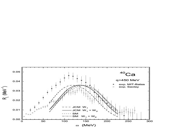
Figure 3: Longitudinal response functions for the ⁴⁰Ca$(e,e^{\prime})$ reaction at $q=450$ MeV$/c$. The contributions of $W_{1}$ and of the sum $W_{1}+W_{2}$ with the ODM of the JCM [41] are displayed together with the SM and SM $W_{1}+W_{2}$ results produced by the phenomenological s.p. wave functions of Ref. [55]. The Saclay data (open squares) are from Ref. [56], the MIT-Bates (black circles) are from Ref. [2].

The longitudinal response functions of the ⁴⁰Ca$(e,e^{\prime})$ reaction at $q=450$ MeV$/c$ is shown in Fig. 3. The JCM $W_{1}$ and JCM $W_{1}+W_{2}$ results are compared with the SM and SM $W_{1}+W_{2}$ ones and with the available data [56, 2]. The main difference between the different results is in the position of the maximum. The contribution of $W_{2}$ shifts the response by $\sim$ 15 MeV at larger values of the energy transfer. The difference between the SM $W_{1}+W_{2}$ and SM results and between the JCM $W_{1}+W_{2}$ and SM $W_{1}+W_{2}$ results indicates the sensitivity of the position of the peak to the different prescriptions used for the energy shifts and to the values of $\epsilon_{n}$ used in the calculations. These effects are more important in a heavier nucleus like ⁴⁰Ca than in ¹⁶O. In comparison with data, our results are closer to the Saclay data.

7 Summary and conclusions

In this paper we have presented a completely antisymmetrized Green’s function approach to inclusive quasielastic electron scattering. The main goals are the following.

i) To express the final state interaction in terms of the self-energy, rather than in terms of the Feshbach optical potential as was done in previous papers, since the mass operator is more closely related to the empirical optical-model potentials. Therefore, we have developed a theoretical approach based on extended projection operators, as in Ref. [18].

ii) To include an approximated treatment of the interference between different reaction channels, which is usually disregarded. This has required some modifications of the treatment of Ref. [18], resulting in a different separation of the hadronic tensor into a direct and an interference part. The latter one is essential to explain the replacement of the self-energy with the empirical potential.

iii) To separate the elastic and inelastic contributions to the hadronic tensor, in order to introduce different approximations concerning the dependence on the state of the residual nucleus.

iv) To include in the calculation the effects of correlations in the target nucleus through the use of a realistic one-body density matrix.

The method has been applied to the reactions ¹⁶O($e,e^{\prime}$) and ⁴⁰Ca($e,e^{\prime}$). Results produced by density matrices including short-range as well as tensor correlations have been compared. The effects of short range correlations are small (within $\sim 5\%$) and within the range of uncertainty related to the choice of other ingredients of the calculation (e.g. the s.p. wave functions). This result is in substantial agreement with previous investigations [10], but a similar effect is found in the present work on the longitudinal and the transverse response functions. Stronger effects are obtained when also tensor correlations are included. For the ¹⁶O($e,e^{\prime}$) reaction at $q=450$ MeV$/c$ the height of the peak is reduced by $\sim 10\%$ when both types of correlations are considered. A correction dependent on the s.p. energies is necessary [the term $W_{2}$ in Eq. (170)] in order to determine the position of the peak. The comparison of the present results with the available experimental data for the nucleus ⁴⁰Ca gives a better agreement, in the longitudinal response, with the Saclay data than with the MIT-Bates ones.

In order to get deeper insight into the dependence of the inclusive electron scattering on correlations, one should also compute the contribution of two-body currents and their interference with tensor correlations, that seems to give a larger effect[12, 9, 13]. In order to accomplish this task, however, a new approach, based on the two-particle Green’s function and including the two-body density matrix, should be developed.

Appendix A APPENDIX

A real number $a$ belongs to the continuous spectrum of a self-adjoint operator $A$ if and only if:

i) it does not belong to the discrete spectrum,

ii) for every $\eta>0$, one can find a normalizable vector $|\psi_{a,\eta}\rangle$ and a constant $C_{a}$ such that

$$\|(a-A)|\psi_{a,\eta}\rangle\|^{2}\leq C_{a}\||\psi_{a,\eta}\rangle\|^{2}\eta.$$ (183)

The vectors $|\psi_{a,\eta}\rangle$ are called “approximate eigenvectors of $A$ related to the eigenvalue $a$” [see Sec. 8.1 of Ref [57]]. Now, we construct a set of approximate eigenvectors of the Hamiltonian $H$ of the residual nucleus, which, added to the exact bound eigenvectors $|n\rangle$, satisfy a completeness relation in the limit $\eta\rightarrow+0$. We remark that this property is not an automatic consequence of Eq. (183).

Let $\mbox{$\mathcal{H}$}_{c}$ be the Hilbert subspace spanned by the non-normalizable eigenvectors $|\epsilon\rangle$ of the continuous spectrum of $H$ which, for simplicity, is assumed to coincide with $[0,+\infty)$. Let $\{|u_{k}\rangle\}$ be a basis in $\mbox{$\mathcal{H}$}_{c}$ consisting of normalizable vectors such that $\langle\epsilon|u_{k}\rangle$ are functions of $\epsilon$ bounded, continuous, and everywhere different from zero. This can be realized weighing the eigenvectors $|\epsilon\rangle$ by means of a complete orthonormal set of functions having the same properties. We set

$$|\epsilon,k;\eta\rangle\equiv\sqrt{\frac{\eta}{\pi}}(\epsilon-H+i\eta)^{-1}|u_{k}\rangle.$$ (184)

Note that the vectors $|\epsilon,k;\eta\rangle$ and $|n\rangle$ are orthogonal.

Theorem 1. The vectors $|\epsilon,k;\eta\rangle$ are approximate eigenvectors of $H$.

Proof. One has

$$\lim_{\eta\rightarrow+0}\||\epsilon,k;\eta\rangle\|^{2}=|\langle\epsilon|u_{k}\rangle|^{2}\neq 0$$ (185)

since

$$\||\epsilon,k;\eta\rangle\|^{2}=\int_{0}^{\infty}{\rm\,d}\,\epsilon^{\prime}L(\epsilon-\epsilon^{\prime};\eta)|\langle\epsilon^{\prime}|u_{k}\rangle|^{2}\,,\,L(x;\eta)\equiv\frac{\eta}{\pi}\frac{1}{x^{2}+\eta^{2}},$$ (186)

and, in the distributional sense of the limit,

$$\lim_{\eta\rightarrow+0}L(x;\eta)=\delta(x).$$ (187)

Moreover, the following inequality holds:

$$\|(\epsilon-H)|\epsilon,k;\eta\rangle\|^{2}=\frac{\eta}{\pi}\langle u_{k}|\frac{(\epsilon-H)^{2}}{(\epsilon-H)^{2}+\eta^{2}}|u_{k}\rangle\leq\frac{\eta}{\pi}\langle u_{k}|u_{k}\rangle=\frac{\eta}{\pi}.$$ (188)

Therefore, one has

$$\lim_{\eta\rightarrow+0}\frac{\|(\epsilon-H)|\epsilon,k;\eta\rangle\|^{2}}{\||\epsilon,k;\eta\rangle\|^{2}}=0$$ (189)

and Eq. (183) is satisfied. $\square$

Theorem 2. In the limit for $\eta\rightarrow+0$, one has the completeness relation

$$\sum_{n}|n\rangle\langle n|+\lim_{\eta\rightarrow+0}\sum_{k}\int_{0}^{\infty}{\rm\,d}\epsilon\,|\epsilon,k;\eta\rangle\langle\epsilon,k;\eta|=1,$$ (190)

where the convergence is understood in the weak sense, i.e., inside a scalar product between normalizable states.

Proof. Due to the orthogonality between the vectors $|\epsilon,k;\eta\rangle$ and $|n\rangle$, it is sufficient to prove Eq. (190) inside the scalar product between vectors $|\phi\rangle$ and $|\chi\rangle$ belonging to $\mbox{$\mathcal{H}$}_{c}$, where both states $\{|\epsilon\rangle\}$ and $\{|u_{k}\rangle\}$ are complete. Thus the sum over $n$ does not contribute, and one considers only

$$\sum_{k}\int_{0}^{\infty}{\rm\,d}\epsilon\,\langle\phi|\epsilon,k;\eta\rangle\langle\epsilon,k;\eta|\chi\rangle=\frac{\eta}{\pi}\int_{0}^{\infty}{\rm\,d}\epsilon\,\langle\phi|\frac{1}{(\epsilon-H)^{2}+\eta^{2}}|\chi\rangle$$

$$=\int_{0}^{\infty}{\rm\,d}\epsilon\,\int_{0}^{\infty}{\rm\,d}\epsilon^{\prime}\,L(\epsilon-\epsilon^{\prime};\eta)\langle\phi|\epsilon^{\prime}\rangle\langle\epsilon^{\prime}|\chi\rangle$$

$$=\int_{0}^{\infty}{\rm\,d}\epsilon^{\prime}\,\langle\phi|\epsilon^{\prime}\rangle\langle\epsilon^{\prime}|\chi\rangle\int_{-\epsilon^{\prime}}^{\infty}{\rm\,d}x\,L(x;\eta),$$ (191)

where in the last step we have exchanged the integrals, according to the Fubini theorem, since $|L(\epsilon-\epsilon^{\prime};\eta)\langle\phi|\epsilon^{\prime}\rangle\langle\epsilon^{\prime}|\chi\rangle|$ is Lebesgue summable in $\epsilon$ and $\epsilon^{\prime}$. Observing that

$$|\langle\phi|\epsilon^{\prime}\rangle\langle\epsilon^{\prime}|\chi\rangle\int_{-\epsilon^{\prime}}^{\infty}{\rm\,d}x\,L(x;\eta)| < \,|\langle\phi|\epsilon^{\prime}\rangle\langle\epsilon^{\prime}|\chi\rangle\int_{-\infty}^{\infty}{\rm\,d}x\,L(x;\eta)|$$ (192)

$$= \langle\phi|\epsilon^{\prime}\rangle\langle\epsilon^{\prime}|\chi\rangle,$$

where the last term is Lebesgue summable and does not depend on $\eta$, we can use the dominated convergence theorem to take the limit for $\eta\rightarrow+0$ within the first integral of the last term in Eq. (191). Thus, using Eq. (187), one obtains

$$\lim_{\eta\rightarrow+0}\sum_{k}\int_{0}^{\infty}{\rm\,d}\epsilon\,\langle\phi|\epsilon,k;\eta\rangle\langle\epsilon,k;\eta|\chi\rangle=\int_{0}^{\infty}{\rm\,d}\epsilon^{\prime}\,\langle\phi|\epsilon^{\prime}\rangle\langle\epsilon^{\prime}|\chi\rangle\int_{-\epsilon^{\prime}}^{\infty}{\rm\,d}x\,\delta(x)$$

$$=\int_{0}^{\infty}{\rm\,d}\epsilon^{\prime}\,\langle\phi|\epsilon^{\prime}\rangle\langle\epsilon^{\prime}|\chi\rangle=\langle\phi|\chi\rangle\,,\,\forall\,|\phi\rangle,|\chi\rangle\in\mbox{$\mathcal{H}$}_{c}.\quad\square$$ (193)

Substituting the completeness relation of Eq. (53) by (190) and introducing the projection operators

$$P(\epsilon,k;\eta)\equiv\int{\rm\,d}\mbox{\boldmath$p$}\,\alpha_{\mathbf{p}}|\epsilon,k;\eta\rangle^{\mathrm{N}}\,{}^{\mathrm{N}}\langle\epsilon,k;\eta|\alpha_{\mathbf{p}}\,,\,|\epsilon,k;\eta\rangle^{\mathrm{N}}\equiv\frac{|\epsilon,k;\eta\rangle}{\||\epsilon,k;\eta\rangle\|},$$ (194)

the contribution of the continuous spectrum is recovered adding to Eq. (64) the term

$$\lim_{\eta\rightarrow+0}\sum_{k}\int{\rm\,d}\epsilon\,\mathrm{Re}\int{\rm\,d}\mbox{\boldmath$p$}{\rm\,d}\mbox{\boldmath$p^{\prime}$}\,\langle\psi_{0}|a_{\mathbf{p-q}}^{\dagger}|\epsilon,k;\eta\rangle$$ (195)

$$\times {}^{\mathrm{N}}\langle\epsilon,k;\eta|\alpha_{\mathbf{p}}\delta(\omega+E_{0}-\epsilon-\hat{H}_{\epsilon})\alpha_{\mathbf{p}^{\prime}}|\epsilon,k;\eta\rangle^{\mathrm{N}}\,\,\langle\epsilon,k;\eta|a_{\mathbf{p}^{\prime}}J^{0}(\mbox{\boldmath$q$})|\psi_{0}\rangle,$$

where $\hat{H}_{\epsilon}$ is defined analogously to $\hat{H}_{n}$ (see Eq. (25)), i.e. as

$$\hat{H}_{\epsilon}=H-\epsilon\quad\mathrm{in}\quad\mbox{$\mathcal{H}$}^{(Z+1)}\quad,\quad\hat{H}_{\epsilon}=\epsilon-H\quad\mathrm{in}\quad\mbox{$\mathcal{H}$}^{(Z-1)}.$$ (196)

Thus, using the approximation

$${}^{\mathrm{N}}\langle\epsilon,k;\eta|\alpha_{\mathbf{p}}\delta(\omega+E_{0}-\epsilon-\hat{H}_{\epsilon})\alpha_{\mathbf{p}^{\prime}}|\epsilon,k;\eta\rangle^{\mathrm{N}}\simeq\langle\mbox{\boldmath$p$}|\mbox{$\mathcal{S}$}_{0}(\omega+E_{0}-\epsilon_{0}-\tilde{\epsilon})|\mbox{\boldmath$p^{\prime}$}\rangle,$$ (197)

analogous to Eq. (78), and using again Eq. (190) one recovers Eqs. (81)–(86).

References

- [1] S. Boffi, C. Giusti, F. D. Pacati, and M. Radici, Electromagnetic Response of Atomic Nuclei, Oxford Studies in Nuclear Physics, Vol. 20, Clarendon Press, Oxford, 1996; S. Boffi, C. Giusti, and F. D. Pacati, Phys. Rep. 226 (1993) 1.
- [2] C. F. Williamson, et al., Phys. Rev. C 56 (1997) 3152.
- [3] M. Anghinolfi, et al., Nucl. Phys. A602, (1996) 405.
- [4] J. P. Chen, S. Choi, and Z. E. Meziani, spokespersons, JLab experiment E-01-016.
- [5] V. Van der Sluys, J. Ryckebusch, and M. Waroquier, Phys. Rev. C 51, (1995) 2664.
- [6] R. Cenni, F. Conte, and P. Saracco, Nucl. Phys. A623, (1997) 391.
- [7] J. E. Amaro, M. B. Barbaro, J. A. Caballero, T. W. Donnelly, and A. Molinari, Phys. Rep. 368, (2002) 317; Nucl. Phys. A723 (2003) 181.
- [8] J. E. Amaro, M. B. Barbaro, J. A. Caballero, and F. Kazemi Tabatabaei, Phys. Rev. C 68 (2003) 014604.
- [9] A. Fabrocini, Phys. Rev. C 55 (1997) 338.
- [10] G. Co’ and A. M. Lallena, Ann. Phys. 287 (2001) 101.
- [11] A. Meucci, F. Capuzzi, C. Giusti, and F. D. Pacati, Phys. Rev. C 67 (2003) 054601.
- [12] W. Leidemann and G. Orlandini, Nucl. Phys. A506 (1990) 447.
- [13] I. Sick, in Nuclear Theory, Heron Press Science Series, Sofia, 2002, p. 16.
- [14] Y. Horikawa, F. Lenz, and N. C. Mukhopadhyay, Phys. Rev. C 22 (1980) 1680.
- [15] C. R. Chinn, A. Picklesimer, and J. W. Van Orden, Phys. Rev. C 40 (1989) 790; Phys. Rev. C 40 (1989) 1159.
- [16] P. M. Boucher and J. W. Van Orden, Phys. Rev. C 43 (1991) 582.
- [17] F. Capuzzi, C. Giusti, and F. D. Pacati, Nucl. Phys. A524 (1991) 681.
- [18] F. Capuzzi and C. Mahaux, Ann. Phys. (N.Y.) 254 (1997) 130.
- [19] H. Feshbach, Ann. Phys. (N.Y.) 5 (1958) 357.
- [20] H. Feshbach, Ann. Phys. (N.Y.) 19 (1962) 287.
- [21] F. Capuzzi and C. Mahaux, Ann. Phys. (N.Y.) 245 (1996) 147.
- [22] A. Fabrocini and S. Fantoni, Nucl. Phys. A503 (1989) 375.
- [23] J. Jourdan, Nucl. Phys. A603 (1996) 117.
- [24] H. Feshbach, Theoretical Nuclear Physics: Nuclear Reactions, Wiley, New York, 1992, and references contained therein.
- [25] E. J. Moniz, Phys. Rev. 184 (1969) 1154.
- [26] E. J. Moniz, I. Sick, R. R. Whitney, J. R. Ficenec, R. D. Kephart, and W. P. Trower, Phys. Rev. Lett. 26 (1971) 445.
- [27] W. Tornow, Z. P. Chen, and J. P. Delaroche, Phys. Rev. C 42 (1990) 693 .
- [28] F. Capuzzi, Nucl. Phys. A554 (1993) 362.
- [29] O. Benhar, A. Fabrocini, S. Fantoni, G. A. Miller, V. R. Pandharipande, and I. Sick, Phys. Rev. C 44 (1991) 2328.
- [30] C. Ciofi degli Atti and S. Simula, Phys. Lett. B 325 (1994) 276.
- [31] O. Benhar, A. Fabrocini, S. Fantoni, and I. Sick, Nucl. Phys. A 579 (1994) 493.
- [32] I. Sick, S. Fantoni, A. Fabrocini, and O. Benhar, Phys. Lett. B 323 (1994) 267.
- [33] O. Benhar, A. Fabrocini, S. Fantoni, and I. Sick, Phys. Lett. B 343 (1995) 47.
- [34] O. Benhar, A. Fabrocini, S. Fantoni, V. R. Pandharipande, S. C. Pieper, and I. Sick, Phys. Lett. B 359 (1995) 8.
- [35] C. Mahaux, P. F. Bortignon, R. A. Broglia, and C. H. Dasso, Phys. Rep. 120 (1985) 1.
- [36] F. Capuzzi and C. Mahaux, Ann. Phys. (N.Y.) 239 (1995) 57.
- [37] F. G. Perey and B. Buck, Nucl. Phys. 32 (1962) 353.
- [38] F. Capuzzi, in Nuclear Optical Model Potential, Lecture Notes in Physics, Vol. 55, eds. J. Ehlers, et al., Springer, Berlin, 1976, p. 20.
- [39] H. Fiedeldey, Nucl. Phys. 77 (1966) 149.
- [40] P. - O. Löwdin, Phys. Rev. 97 (1955) 1474.
- [41] M. V. Stoitsov, A. N. Antonov, and S. S. Dimitrova, Phys. Rev. C 47 (1993) R455; Phys. Rev. C 48 (1993) 74; Z. Phys. A 345 (1993) 359.
- [42] D. Van Neck, L. Van Daele, Y. Dewulf, and M. Waroquier, Phys. Rev. C 56 (1997) 1398.
- [43] A. Polls, H. Müther and W. H. Dickhoff, Proceedings of Conference on Perspectives in Nuclear Physics at Intermediate Energies, Trieste, 1995, edited by S. Boffi, C. Ciofi degli Atti, and M.M. Giannini, World Scientific, Singapore, 1996, p. 308.
- [44] R. Jastrow, Phys. Rev. 98 (1955) 1479.
- [45] M. Gaudin, J. Gillespie, and G. Ripka, Nucl. Phys. A176 (1971) 237; M. Dal Rí, S. Stringari, and O. Bohigas, Nucl. Phys. A376 (1982) 81.
- [46] S. C. Pieper, R. B. Wiringa, and V. R. Pandharipande, Phys. Rev. C 46 (1992) 1741.
- [47] W. H. Dickhoff and H. Müther, Rep. Prog. Phys. 55 (1992) 1947.
- [48] H. Müther, A. Polls, and W. M. Dickhoff, Phys. Rev. C 51 (1995) 3040; H. Müther, G. Knehr, and A. Polls, Phys. Rev. C 52 (1995) 2955.
- [49] M. V. Stoitsov, A. N. Antonov, and S. S. Dimitrova, Phys. Rev. C 53 (1996) 1254.
- [50] M. K. Gaidarov, K. A. Pavlova, S. S. Dimitrova, M. V. Stoitsov, A. N. Antonov, D. Van Neck, and H. Muether, Phys. Rev. C 60 (1999) 024312.
- [51] D. Van Neck, M. Waroquier, and K. Heyde, Phys. Lett. B 314 (1993) 255.
- [52] C. Giusti and F. D. Pacati, Nucl. Phys. A473 (1987) 717; Nucl. Phys. A485 (1988) 461.
- [53] K. W. McVoy and L. Van Hove, Phys. Rev. 125 (1962) 1034.
- [54] P. Schwandt, H. O. Meyer, W. W. Jacobs, A. D. Bacher, S. E. Vigdor, M. D. Kaitchuck, and T. R. Donoghue, Phys. Rev. C 26 (1982) 55.
- [55] L. R. B. Elton and A. Swift, Nucl. Phys. A94 (1967) 52.
- [56] Z. E. Meziani, et al., Phys. Rev. Lett. 52 (1984) 2130; 54 (1985) 1233.
- [57] R. D. Richtmyer, Principles of Advanced Mathematical Physics, Vol. 1, Springer-Verlag, New York, 1978.