Deuteron Compton Scattering in Effective Field Theory:
Spin-Dependent Cross Sections and Asymmetries

Abstract

Polarized Compton scattering on the deuteron is studied in nuclear effective field theory. A set of tensor structures is introduced to define 12 independent Compton amplitudes. The scalar and vector amplitudes are calculated up to ${\cal O}((Q/\Lambda)^{2})$ in low-energy power counting. Significant contribution to the vector amplitudes is found to come from the spin-orbit type of relativistic corrections. A double-helicity dependent cross section $\Delta_{1}\sigma=\left(\sigma_{+1-1}-\sigma_{+1+1}\right)/2$ is calculated to the same order, and the effect of the nucleon isoscalar spin-dependent polarizabilities is found to be smaller than the effect of isoscalar spin-independent ones. Contributions of spin-independent polarizabilities are investigated in various asymmetries, one of which has as large as 12 (26) percent effect at the center-of-mass photon energy 30 (50) MeV.

I Introduction

Compton scattering is an important tool to probe the internal structure of a composite system, such as an atomic nuclei. As quantum electrodynamics involved in the process is well understood, the remaining uncertainty is associated with the strong interactions among nucleons in nuclei. Thus Compton scattering data enables physicists to extract information about the nuclear structure from the underlying strong interaction dynamics. Recent progress in high-energy, high-intensity photon beams has made Compton scattering a practical tool for nuclear physicists higs . In particular, a polarized photon beam is capable of studying spin aspects of strong interaction physics. This paper focuses on polarized Compton scattering on the deuteron, the double-helicity dependent cross section in particular, in the framework of nuclear effective field theory (EFT).

The deuteron, as the simplest nuclear system, is of great importance for understanding the nucleon-nucleon interactions and the properties of individual nucleons. Polarized Compton scattering on the deuteron presents a new opportunity to probe spin physics. Indeed, because the deuteron is a loosely bound system, one might expect to learn a host of spin-dependent properties of the neutron and proton as free particles. This possibility is especially important for the structure of the neutron because there is no free neutron target in nature.

It has been realized for some time that nuclear physics at low energy might be understood by effective field theories (EFT) which works according to the same principles as the standard model weinberg . However, constructing a workable scheme for specific systems is not straightforward. In the past few years, considerable progress has been made in the two-nucleon sector (see review for a recent review). It began with the pioneering work of Weinberg, who proposed to encode the short-distance physics in a derivative expansion of local operators weinberg . The problem associated with the unusually small binding energy of the deuteron was solved by Kaplan, Savage and Wise by exploiting the freedom of choosing a renormalization substraction scheme kaplan1 , quickly followed by the pionless version chen1 (see also vK97 ; Cohen97 ; BHvK1 ). Required reproducing the residue of the deuteron pole at next-to-leading order (NLO), a version with accelerated convergence was suggested in phillips . The use of dibaryon fields as auxiliary fields, first introduced in kaplan2 , was taken seriously in savage which simplified the calculation significantly.

From the viewpoint of nuclear EFT, Compton scattering on the deuteron at low energy can be divided into two regions according to the photon energy $\omega$. Region I is where the photon energy is far below the binding energy of deuteron $B=2.2$ MeV and, hence, $\omega/B$ is a small parameter. Region II is where the photon energy is above the binding energy, but significantly below the mass of the pion, for example, $\omega\sim$ 50 MeV. In Region I, one makes the low energy expansion of Compton amplitudes and studies various polarizabilities of the deuteron defined through the expansion Ji . Studies in this ultra-low energy region, where the binding effect plays a dominant role, provide insight about the internal structure of the deuteron as a bound state. In Region II, the probing photon is more sensitive to the responses from individual nucleons. Therefore, Compton scattering there may serve as an alternative tool to study free-nucleon properties, such as spin-independent and dependent polarizabilities. In this paper, we are mostly interested in the second region.

Extracting the isoscalar spin-independent polarizabilities $\alpha_{0}$ and $\beta_{0}$ from unpolarized Compton scattering has attracted considerable attention in the past two decades. Although there are three types of amplitudes (scalar, vector and tensor) contributing to the cross section, only the scalar amplitudes have been included in some of the calculations of the unpolarized cross section so far. Nuclear EFT seems to provide a justification for this. However, a recent work unpolarized showed that vector amplitudes contribute significantly (order of 15% or more) to the unpolarized cross section, because of the enhancement from a factor of the square of the isovector magnetic moment $\mu^{2}_{1}$. It turns out that this enhancement has its effect not only on unpolarized scattering but also on polarized one, leading to, for instance, a bigger helicity-dependent cross section. Although this makes it easier to measure it experimentally, the effect also diminishes the contribution from the isoscalar nucleon spin-dependent polarizabilities, and hence makes it harder to access them from the future Compton data.

To demonstrate the above point, we calculate a double-helicity dependent (vector-polarized) cross section up to the order at which the spin polarizabilities contribute, and compare the results with and without their contribution. The photon-nucleon interactions considered in this calculation include the electric current and magnetic couplings, and the spin-orbit terms from the non-relativistic reduction of the relativistic interactions. It has been realized previously that the relativistic corrections are surprisingly large in potential model calculations weyrauch ; wilbois ; levchuk ; lvov ; karakowski . In EFT, the spin-orbit interactions were taken into account in the studies of the deuteron forward spin-dependent polarizabilities Ji and Drell-Hearn-Gerasimov sum rule DHG . They were neglected in other EFT calculations because they are nominally suppressed in power counting by $1/M_{N}$ relative to the other two couplings. However, for certain spin-dependent observables, their contributions can be of leading order, as we shall see.

The paper is organized as follows. Section II is devoted to kinematics, where we write down 12 basis structures for scattering amplitudes using parity and time-reversal symmetries. The scalar and vector structures are the same as those in Compton scattering on a spin-1/2 particle such as the proton. The tensor structures are new, and useful for general discussions of polarized deuteron Compton scattering. Section III explains a calculation of the vector Compton amplitudes using the dibaryon formulation of EFT. Power counting in both Regions I and II is explained to show the significant contribution of the spin-orbit interactions. The result of individual diagrams is listed in Appendix B. In Sec. IV, a double-helicity-dependent (vector-polarized) cross section is defined, and the numerical result is presented with and without the contribution from the nucleon spin-dependent polarizabilities. The feasibility of using polarized Compton data to extract these polarizabilities is discussed. In Sec. V, we investigate the effect of the spin-independent polarizabilities on a number of spin asymmetries. Section VI contains the conclusion of the paper.

II Real Photon-Deuteron Compton Scattering Amplitudes

In this section, the general tensor structure of the amplitudes for real photon Compton scattering on a deuteron is considered. Through helicity counting, it is easy to see that there are a total of 12 independent amplitudes. We choose these amplitudes in a basis convenient for subsequent calculations. We comment on the frame dependence of the tensor structures associated with the amplitudes.

The real photon has two independent helicities $\pm 1$; the deuteron has three, $\pm 1$ and 0. Therefore, the total number of helicity amplitudes is $2\times 3\times 2\times 3=36$. Parity invariance of strong and electromagnetic interactions restricts the number of independent ones to 36/2=18. Among those, time-reversal symmetry relates 6 to the others with initial and final state exchanged. This reduces the number of independent amplitudes to $18-6=12$. Moreover, the general result of helicity counting can be derived, and is $2(J+1)(2J+1)$ for a spin-$J$ target.

In the low-energy region, it is convenient to use the nonrelativistic notation for tensor structures associated with the amplitudes. If the spins of the initial and final deuterons are coupled, the sum is 0, 1 or 2. The amplitudes classified in this way are called scalar, vector, and tensor, respectively. Clearly the number of scalar amplitudes must be the same as that of Compton scattering amplitudes on a spin-0 target, namely, 2; and the number of vector amplitudes is the same as that on a spin-1/2 target, 4. Thus the number of independent tensor amplitudes is $12-2-4=6$.

In the remainder of this section, we construct a set of 12 linearly-independent structures, using the 3-momenta of the photon and deuteron, and their polarization vectors. Among four 3-momenta, only three are independent because of the momentum conservation. By choosing a specific frame, one more constraint follows, and hence only initial and final 3-momenta of photon, $\vec{k}$ and $\vec{k}^{\prime}$, are needed for the construction. The initial and final three-momenta of the deuteron, $\vec{p}$ and $\vec{p}^{\prime}$ can be expressed in terms of these of the photon. For example, the lab frame is defined by $\vec{p}=0$ and $\vec{p}^{\prime}=\vec{k}-\vec{k}^{\prime}$, the center-of-mass frame (CM) by $\vec{p}=-\vec{k}$ and $\vec{p}^{\prime}=-\vec{k}^{\prime}$, and the so-called Breit frame by $\vec{p}=\frac{1}{2}(\vec{k}^{\prime}-\vec{k})$ and $\vec{p}^{\prime}=-\frac{1}{2}(\vec{k}^{\prime}-\vec{k})$ and so $\vec{p}+\vec{p}^{\prime}=0$. The constraints among momenta associated with a frame are generally not invariant under symmetries such as time reversal, which exchanges the initial and final momenta and reverses their directions, and photon crossing symmetry, which exchanges the initial and final photon with the sign of energy and 3-momentum flipped. For instance, the momentum constraint in the lab frame is not invariant under either time reversal or crossing symmetry, while the momentum constraint in the CM frame violates crossing symmetry.

According to the above, in the CM and Breit frames where parity and time reversal invariance are manifest, there are 12 independent tensor structures for the Compton amplitudes. These structures are constructed out of initial and final photon polarization vectors ($\hat{\epsilon}^{\prime*}$ and $\hat{\epsilon}$), deuteron polarization vectors ($\hat{\xi}^{\prime*}$ and $\hat{\xi}$), and the initial and final photon momentum vectors $\hat{k}={\vec{k}}/{|\vec{k}|}$ and $\hat{k}^{\prime}={\vec{k}^{\prime}}/{|\vec{k}^{\prime}|}$. One can couple ($\hat{\xi}^{\prime*}$ and $\hat{\xi}$) into scalar, vector and tensor to obtain scalar, vector, and tensor amplitudes. Alternatively, these structures can be obtained by the matrix element of a unit matrix $I$, spin matrices $J_{i}$, or tensor $(J_{i}J_{j}+J_{j}J_{i}-{\rm trace})$ between the initial and final deuteron polarization vectors. Under parity transformation, all momentum and polarization vectors change sign, whereas the spin matrices do not. Under time-reversal transformation, these quantities transform according to: $\hat{\epsilon}\Leftrightarrow\hat{\epsilon}^{\prime*};\*\*\hat{k}\Leftrightarrow-\hat{k}^{\prime};\vec{J}\Rightarrow-\vec{J}$.

Requiring symmetry under both parity and time-reversal, we choose the 12 basis structures for Compton scattering on the deuteron as follows,

$$\rho_{1} = \hat{\epsilon}^{\prime\ast}\cdot\hat{\epsilon}\;I=\epsilon^{\prime\ast}\cdot\hat{\epsilon}\;\xi^{\prime\ast}\cdot\xi~{},$$

$$\rho_{2} = \hat{s}^{\prime*}\cdot\hat{s}\;I=\hat{s}^{\prime*}\cdot\hat{s}\;\xi^{\prime\ast}\cdot\xi~{},$$

$$\rho_{3} = iJ\cdot\hat{\epsilon}^{\prime\ast}\times\hat{\epsilon}=(\xi^{\prime\ast}\times\xi)\cdot(\hat{\epsilon}^{\prime\ast}\times\hat{\epsilon})~{},$$

$$\rho_{4} = iJ\cdot\hat{s}^{\prime*}\times\hat{s}=(\xi^{\prime\ast}\times\xi)\cdot(\hat{s}^{\prime*}\times\hat{s})~{},$$

$$\rho_{5} = i(J\cdot\hat{k}\hat{s}^{\prime*}\cdot\hat{\epsilon}-J\cdot\hat{k}^{\prime}\hat{\epsilon}^{\prime\ast}\cdot\hat{s})=[(\xi^{\prime\ast}\times\xi)\cdot\hat{k}\hat{s}^{\prime*}\cdot\hat{\epsilon}-(\xi^{\prime\ast}\times\xi)\cdot\hat{k}^{\prime}\hat{\epsilon}^{\prime\ast}\cdot\hat{s}]~{},$$

$$\rho_{6} = i(J\cdot\hat{k}^{\prime}\hat{s}^{\prime*}\cdot\hat{\epsilon}-J\cdot\hat{k}\hat{\epsilon}^{\prime\ast}\cdot\hat{s})=[(\hat{\xi}^{\prime*}\times\hat{\xi})\cdot\hat{k}^{\prime}\hat{s}^{\prime*}\cdot\hat{\epsilon}-(\xi^{\prime\ast}\times\xi)\cdot\hat{k}\hat{\epsilon}^{\prime\ast}\cdot\hat{s}]~{},$$

$$\rho_{7} = -(J\cdot\hat{\epsilon}J\cdot\hat{\epsilon}^{\prime*}+J\cdot\hat{\epsilon}^{\prime*}J\cdot\hat{\epsilon}-\frac{4}{3}\hat{\epsilon}^{\prime*}\cdot\hat{\epsilon})=\hat{\xi}^{\prime*}\cdot\hat{\epsilon}^{\prime*}\hat{\xi}\cdot\hat{\epsilon}+\hat{\xi}^{\prime*}\cdot\hat{\epsilon}\hat{\xi}\cdot\hat{\epsilon}^{\prime*}-\frac{2}{3}\hat{\xi}^{\prime*}\cdot\hat{\xi}\hat{\epsilon}^{\prime*}\cdot\hat{\epsilon}~{},$$

$$\rho_{8} = -(J\cdot\hat{s}J\cdot\hat{s}^{\prime*}+J\cdot\hat{s}^{\prime*}J\cdot\hat{s}-\frac{4}{3}\hat{s}^{\prime*}\cdot\hat{s})=\hat{\xi}^{\prime*}\cdot\hat{s}^{\prime*}\hat{\xi}\cdot\hat{s}+\hat{\xi}^{\prime*}\cdot\hat{s}\hat{\xi}\cdot\hat{s}^{\prime*}-\frac{2}{3}\hat{\xi}^{\prime*}\cdot\hat{\xi}\hat{s}^{\prime*}\cdot\hat{s}~{},$$

$$\rho_{9} = -\hat{\epsilon}^{\prime*}\cdot\hat{k}(J\cdot\hat{\epsilon}J\cdot\hat{k}^{\prime}+J\cdot\hat{k}^{\prime}J\cdot\hat{\epsilon})-\hat{\epsilon}\cdot\hat{k}^{\prime}(J\cdot\hat{\epsilon}^{\prime*}J\cdot\hat{k}+J\cdot\hat{k}J\cdot\hat{\epsilon}^{\prime*})+\frac{8}{3}\hat{\epsilon}^{\prime*}\cdot\hat{k}\hat{\epsilon}\cdot\hat{k}^{\prime}$$

$$= \hat{\epsilon}^{\prime*}\cdot\hat{k}(\hat{\xi}^{\prime*}\cdot\hat{k}^{\prime}\hat{\xi}\cdot\hat{\epsilon}+\hat{\xi}^{\prime*}\cdot\hat{\epsilon}\hat{\xi}\cdot\hat{k}^{\prime})+\hat{\epsilon}\cdot\hat{k}^{\prime}(\hat{\xi}^{\prime*}\cdot\hat{k}\hat{\xi}\cdot\hat{\epsilon}^{\prime*}+\hat{\xi}^{\prime*}\cdot\hat{\epsilon}^{\prime*}\hat{\xi}\cdot\hat{k})-\frac{4}{3}\hat{\xi}^{\prime*}\cdot\hat{\xi}\hat{\epsilon}^{\prime*}\cdot\hat{k}\hat{\epsilon}\cdot\hat{k}^{\prime}~{},$$

$$\rho_{10} = -\hat{s}^{\prime*}\cdot\hat{k}(J\cdot\hat{s}J\cdot\hat{k}^{\prime}+J\cdot\hat{k}^{\prime}J\cdot\hat{s})-\hat{s}\cdot\hat{k}^{\prime}(J\cdot\hat{s}^{\prime*}J\cdot\hat{k}+J\cdot\hat{k}J\cdot\hat{s}^{\prime*})+\frac{8}{3}\hat{s}^{\prime*}\cdot\hat{k}\hat{s}\cdot\hat{k}^{\prime}$$

$$= \hat{s}^{\prime*}\cdot\hat{k}(\hat{\xi}^{\prime*}\cdot\hat{k}^{\prime}\hat{\xi}\cdot\hat{s}+\hat{\xi}^{\prime*}\cdot\hat{s}\hat{\xi}\cdot\hat{k}^{\prime})+\hat{s}\cdot\hat{k}^{\prime}(\hat{\xi}^{\prime*}\cdot\hat{k}\hat{\xi}\cdot\hat{s}^{\prime*}+\hat{\xi}^{\prime*}\cdot\hat{s}^{\prime*}\hat{\xi}\cdot\hat{k})-\frac{4}{3}\hat{\xi}^{\prime*}\cdot\hat{\xi}\hat{s}^{\prime*}\cdot\hat{k}\hat{s}\cdot\hat{k}^{\prime}~{},$$

$$\rho_{11} = -\hat{\epsilon}^{\prime*}\cdot\hat{\epsilon}(J\cdot\hat{k}J\cdot\hat{k}+J\cdot\hat{k}^{\prime}J\cdot\hat{k}^{\prime}-\frac{4}{3})=\hat{\epsilon}^{\prime*}\cdot\hat{\epsilon}(\hat{\xi}^{\prime*}\cdot\hat{k}\hat{\xi}\cdot\hat{k}+\hat{\xi}^{\prime*}\cdot\hat{k}^{\prime}\hat{\xi}\cdot\hat{k}^{\prime}-\frac{2}{3}\hat{\xi}^{\prime*}\cdot\hat{\xi})~{},$$

$$\rho_{12} = -\hat{s}^{\prime*}\cdot\hat{s}(J\cdot\hat{k}J\cdot\hat{k}+J\cdot\hat{k}^{\prime}J\cdot\hat{k}^{\prime}-\frac{4}{3})=\hat{s}^{\prime*}\cdot\hat{s}(\hat{\xi}^{\prime*}\cdot\hat{k}\hat{\xi}\cdot\hat{k}+\hat{\xi}^{\prime*}\cdot\hat{k}^{\prime}\hat{\xi}\cdot\hat{k}^{\prime}-\frac{2}{3}\hat{\xi}^{\prime*}\cdot\hat{\xi})~{},$$ (1)

where the $\hat{s}$ and $\hat{s}^{\prime*}$ are defined as $\hat{s}=\hat{k}\times\hat{\epsilon}$ and $\hat{s}^{\prime*}=\hat{k}^{\prime}\times\hat{\epsilon}^{\prime*}$. These structures are constructed in such a way that duality between the electric and magnetic fields is manifest. Under the dual transformation, $\hat{\epsilon}\Rightarrow\hat{s}$, $\hat{s}\Rightarrow-\hat{\epsilon}$, which is a $\pi/2$-rotation in the photon polarization, the above structures transform as $\rho_{2i-1}\Leftrightarrow\rho_{2i}$ with $i=1,...,6$. The structures with the unit matrix and spin operators ($\rho_{1}$ to $\rho_{6}$) are the same as those for a spin-1/2 target babusci . Appendix A explains why these 12 structures are complete and independent.

The most general Compton scattering amplitude on the deuteron can be expressed as

$$f=\sum_{i=1}^{12}f_{i}\rho_{i}\ ,$$ (2)

where $f_{i}$ defines the spin-dependent amplitudes. The first two ($i=1,2$) are scalar amplitudes; the following four ($i=3,...,6$) are vector amplitudes; and the last six ($i=7,...,12$) are tensor amplitudes.

III Vector Compton Amplitudes to $(Q/\Lambda)^{4}$ from EFT

In this section, we calculate the vector Compton amplitudes to $(Q/\Lambda)^{4}$ in a low-energy expansion in nuclear EFT. The calculation is based on the dibaryon approach in the pionless theory, which has been referred as dEFT($\not\!\pi$) savage .

A central concept in EFT is power counting. EFT is designed to describe physics at one scale—low-energy scale in this case—using an effective lagrangian, and the physics at other scales is accounted for through the couplings. Power counting allows a systematic way to take into account corrections from other energy scales. For Compton scattering on the deuteron, the natural momentum scale is $\sqrt{M_{N}B}$ ($M_{N}$ is the nucleon mass) which will be generically referred to as $Q$. The deuteron binding energy $B$ is then counted as order of $Q^{2}$. The energy and momentum of the external photon probe, $\omega=|\vec{k}|$, is counted as

• $Q^{2}$ in Region I where $\omega\ll B$, and as

• $Q$ in Region II, where $\omega\sim\sqrt{M_{N}B}$.

The high-energy scales include the nucleon mass $M_{N}$, the pion mass $m_{\pi}$, and similar scales describing the structure of the nucleon, like the charge radius, and parameters in nucleon-nucleon interactions. Because $m_{\pi}$ and $M_{N}$ are very different, we use $\Lambda$ to denote scales at around $m_{\pi}$, and identify $m_{\pi}/M_{N}$ as $Q/\Lambda$. Therefore, ratio $Q/M_{N}$ can actually be treated as $(Q/\Lambda)^{2}$. Although this is not fully consistent in the EFT sense, it is a way to organize numerically-close ratios phenomenologically rupak .

In dEFT($\not\!\pi$), the nucleon rescattering in both singlet ${}^{1}S_{0}$ and triplet ${}^{3}S_{1}$ channels is represented by the propagation of dibaryon fields, $t_{j}$ and $s_{a}$, respectively. The lagrangian density for the triplet channel is savage :

$${\cal L}=N^{\dagger}\left[i\partial_{0}+\frac{\mathbf{D}^{2}}{2M_{N}}\right]N-t^{\dagger}_{j}\left[i\partial_{0}+\frac{\mathbf{D}^{2}}{4M_{N}}-\Delta\right]t^{j}-y\left[t^{\dagger}_{j}N^{T}P^{j}N+h.c.\right]~{},$$ (3)

where $N$ is the 2-component nucleon field with an implicit isospin index. The time and spatial derivatives with electromagnetic gauge symmetry are $D_{0}$ and $\mathbf{D}$, respectively. $P^{j}=\frac{1}{\sqrt{8}}\tau_{2}\sigma_{2}\sigma_{j}$ is the projection operator of the triplet channel, and $y$ is the coupling between nucleons in the triplet channel and the triplet dibaryon. Requiring producing the nucleon-nucleon scattering amplitude, one has

$$y^{2}=\frac{8\pi}{M^{2}_{N}r^{(3S_{1})}},~{}~{}~{}\Delta=\frac{2}{M_{N}r^{(3S_{1})}}\left(\frac{1}{a^{(3S_{1})}}-\mu\right)~{},$$ (4)

with $\mu$ being the renormalization-scale introduced in the power divergent subtraction scheme kaplan1 . The parameters $a$ and $r$ are the scattering length and effective range, respectively. In the present formulation, these two are counted as order $Q^{-1}$ in both singlet and triplet channels. Thus the scaling property of $y$ and $\Delta$ is $y\sim\sqrt{Q}$ and $\Delta\sim Q^{2}$, respectively. Dressing the dibaryon propagator with nucleon bubbles does not change the counting of the propagator. Therefore the bubbles must be summed to all orders; the dibaryon propagator dressed with nucleon bubbles is

$$D^{(3S_{1})}\left(\overline{E}\right)=\frac{4\pi}{M_{N}y^{2}}\frac{i}{\mu+\frac{4\pi}{M_{N}y^{2}}\left(\Delta-\overline{E}\right)+i\sqrt{M_{N}\overline{E}}}\ ,$$ (5)

with $\overline{E}$ the center-of-mass energy. The wave function renormalization constant is the residue at pole $\overline{E}=-B$, and a simple calculation yields savage : $z_{d}={\gamma r^{(3S_{1})}}/(1-\gamma r^{(3S_{1})})$  .

We remark that it is straightforward to convert the nuclear EFT lagrangian with the nucleon field into that in dEFT($\not\!\pi$). Following the prescription in savage , one converts a pair of nucleon fields in the singlet and triplet channels to dibaryon fields,

$$N^{T}P^{j}N\rightarrow\frac{1}{\sqrt{M_{N}r^{(3S_{1})}}}t^{j},~{}~{}~{}N^{T}\overline{P}^{a}N\rightarrow\frac{1}{\sqrt{M_{N}r^{(1S_{0})}}}s^{a},$$ (6)

where $\overline{P}^{a}=\frac{1}{\sqrt{8}}\sigma_{2}\tau_{2}\tau_{a}$ is the projection operator for the singlet channel.

Nuclear EFT describes the interactions between the nucleons and external electromagnetic probes systematically. Besides the coupling generated in the covariant derivatives in the above lagrangian density, $\mathbf{D}=\vec{\nabla}-ie\mathbf{A}$, there is also the magnetic coupling to the nucleon,

$${\cal L}_{\rm B}=\frac{e}{2M_{N}}N^{\dagger}(\mu_{0}+\mu_{1}\tau_{3})\mathbf{\sigma}\cdot\mathbf{B}N\ ,$$ (7)

where $\mu_{0}$ and $\mu_{1}$ are the nucleon’s isoscalar and isovector magnetic moments, respectively. An associated term is the spin-orbit-type relativistic correction

$${\cal L}_{\rm SO}=i\frac{e}{8M^{2}_{N}}\left(\left(2\mu_{0}-\frac{1}{2}\right)+\left(2\mu_{1}-\frac{1}{2}\right)\tau_{3}\right)N^{\dagger}\vec{\sigma}\cdot(\mathbf{D}\times\mathbf{E}-\mathbf{E}\times\mathbf{D})N\ ,$$ (8)

which is generated from the reduction of a relevant relativistic interaction.

There are also interaction terms involving the dibaryon fields themselves. One term accounts for the transition between the ${}^{3}S_{1}$ and ${}^{1}S_{0}$ channels through a magnetic field,

$$\mathcal{L}_{\mathrm{em,1}}=e\frac{L_{1}}{M_{N}\sqrt{r^{(^{1}S_{0})}r^{(^{3}S_{1})}}}t_{j}^{\dagger}s_{3}B_{j}+\mathrm{h.c.}~{}.$$ (9)

The coupling constant $L_{1}$ has been determined by the rate of $n+p\rightarrow d+\gamma$. The measured cross section $\sigma=334.2\pm 0.5$ mb with an incident neutron speed of $2200$ m/s fixes $L_{1}=-4.42$ fm. Another term involves the elastic scattering of the deuteron in the magnetic field,

$$\mathcal{L}_{\mathrm{em,2}}=-i\frac{e}{M_{N}}\left(\mu_{0}-\frac{L_{2}}{r^{(^{3}S_{1})}}\right)\varepsilon^{ijk}t_{i}^{\dagger}B_{j}t_{k}\ ,$$ (10)

with the value of $L_{2}$ fixed to be $-0.03$ fm from the magnetic moment of the deuteron. The $\mu_{0}$ in the above equation is introduced to reproduce the magnetic moment at leading order detmold ; ando . There is also an associated relativistic correction,

$$\mathcal{L}_{\mathrm{em,2}}^{\mathrm{SO}}=\frac{e}{2M_{N}^{2}}\left(\mu_{0}-\frac{L_{2}}{r^{(^{3}S_{1})}}-\frac{1}{4}\right)\varepsilon^{ijk}t_{i}^{\dagger}\left(\mathbf{D}\times\mathbf{E}-\mathbf{E}\times\mathbf{D}\right)_{j}t_{k}\ ,$$ (11)

which generates a seagull interaction of the dibaryon and electromagnetic fields. At last, there are nucleon polarizabilities interactions:

$$\mathcal{L}_{\mathrm{pol}} = 2\pi N^{\dagger}\left(\alpha_{0}+\alpha_{1}\tau_{3}\right)\mathbf{E}^{2}N+2\pi N^{\dagger}\left(\beta_{0}+\beta_{1}\tau_{3}\right)\mathbf{B}^{2}N$$ (12)

$$+2\pi N^{\dagger}\left(\gamma^{(s)}_{E1}+\gamma^{(v)}_{E1}\tau_{3}\right)\sigma\cdot\mathbf{E}\times\dot{\mathbf{E}}N+2\pi N^{\dagger}\left(\gamma^{(s)}_{M1}+\gamma^{(v)}_{M1}\tau_{3}\right)\sigma\cdot\mathbf{B}\times\dot{\mathbf{B}}N$$

$$-2\pi N^{\dagger}\left(\gamma^{(s)}_{E2}+\gamma^{(v)}_{E2}\tau_{3}\right)E_{ij}\sigma_{i}\mathbf{B}_{j}N+2\pi N^{\dagger}\left(\gamma^{(s)}_{M2}+\gamma^{(v)}_{M2}\tau_{3}\right)B_{ij}\sigma_{i}\mathbf{E}_{j}N~{},$$

where $E_{ij}=1/2(\nabla_{i}\mathbf{E}_{j}+\nabla_{j}\mathbf{E}_{i})$ and $B_{ij}=1/2(\nabla_{i}\mathbf{B}_{j}+\nabla_{j}\mathbf{B}_{i})$ are the electric and magnetic field gradients. The nucleon isoscalar ($\alpha_{0}$,$\beta_{0}$,$\gamma^{(s)}_{E1,M1,E2,M2}$) and isovector ($\alpha_{1}$,$\beta_{1}$,$\gamma^{(v)}_{E1,M1,E2,M2}$) polarizabilities are defined as, for example, $\alpha_{0}=1/2(\alpha_{p}+\alpha_{n})$ and $\alpha_{1}=1/2(\alpha_{p}-\alpha_{n})$, with similar relations for others. The isoscalar ones are what can be probed in deuteron Compton scattering. Chiral perturbation theory calculations yield GHM :

$$\alpha_{0}=10\beta_{0}=12\times 10^{-4}\rm{fm}^{3},$$

$$\gamma^{(s)}_{E1}=-3.1\times 10^{-4}\rm{fm}^{4},~{}~{}\gamma^{(s)}_{M1}=0.4\times 10^{-4}\rm{fm}^{4},$$

$$\gamma^{(s)}_{E2}=2.1\times 10^{-4}\rm{fm}^{4},~{}~{}\gamma^{(s)}_{M2}=0.6\times 10^{-4}\rm{fm}^{4}.$$ (13)

Feynman diagrams that contribute to the deuteron Compton scattering to $(Q/\Lambda)^{4}$ in power counting are shown in Figs. 1-4. Figure 1 contains diagrams with direct photon-dibaryon interactions. Figure 2 contains the seagull interactions with the nucleon. The diagram 2c actually corresponds to the contribution from electromagnetic polarizabilities of the nucleon. Figure 3 include diagrams without intermediate dibaryon fields. Finally diagrams in Fig. 4 have intermediate singlet and triplet dibaryon propagations.

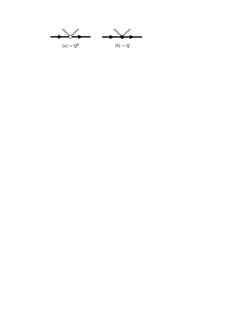
Figure 1: Compton scattering with photons coupled to the dibaryon field directly. The open circle denotes the electric photon-dibaryon coupling from the gauged derivative. The solid dot denotes the seagull term in Eq. (11). The intermediate thick line represents the triplet dibaryon.

0.7

Figure 2: Diagrams with seagull interactions on the nucleon lines. The small open circle denotes the coupling from the gauged derivative in the first term in Eq. (3), the small solid circle represents the coupling from spin-orbit interaction defined in Eq. (8), while the small open box represents the point interactions associated with polarizabilities of the nucleon in Eq. (12). Power counting of the leading contribution of each diagram is listed below the diagram. In diagram 2c, the two countings, $Q$ and $Q^{2}$, are for spin-independent and spin-dependent nucleon polarizabilities contributions, respectively.

0.7

Figure 3: Diagrams without intermediate dibaryons. The small open circles denote the electric photon-nucleon coupling from the gauged derivative in the first term in Eq. (3), the small shaded circles denote the magnetic photon-nucleon coupling in Eq. (7), while the small solid circles represent the spin-orbit interaction between photon and nucleon in Eq. (8).

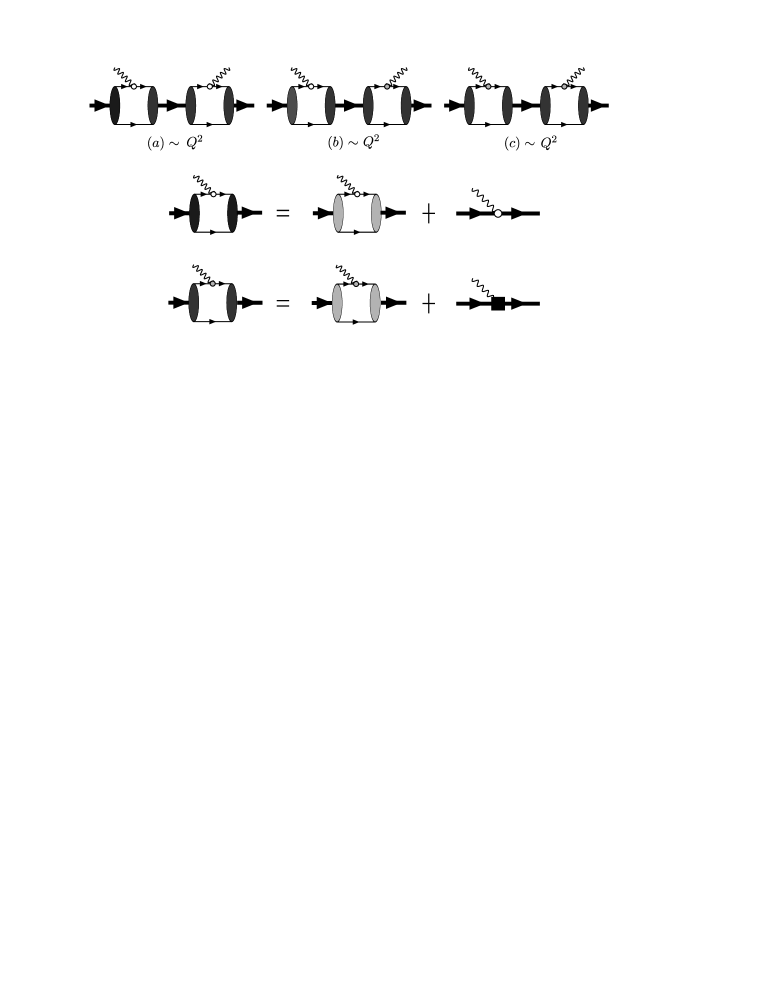
Figure 4: Diagrams with intermediate dibaryon states. The small open circles denote the electric coupling in Eq. (3), and the small shaded circles denote the magnetic coupling in Eq. (7). The intermediate thick lines with one arrow represent both the spin singlet and triplet channels. The solid box denotes the $L_{1}$ and $L_{2}$ couplings in Eqs. (9) and (10).

To estimate the importance of a particular diagram in our power-counting scheme, we need to study the dominant regions of a loop momentum in the integral. Let us use $(q^{0},\vec{q})$ to denote the loop momentum generically. The size of the loop momentum is determined by poles of the propagators. Typical nucleon propagators in the loop integration are ${i}/\left({-B-q_{0}-\frac{\vec{q}^{2}}{2M}+i\varepsilon}\right)$ when the photon momentum does not pass through the nucleon line, and ${i}/\left({q_{0}+\omega-\frac{\vec{q}^{2}}{2M}+i\varepsilon}\right)$ when the photon momentum does. Because $q_{0}$ scales as $|\vec{q}|^{2}$, the former has a momentum pole at $|\vec{q}|\sim\sqrt{B}$ and the latter a pole at $|\vec{q}|\sim\sqrt{\omega}=\sqrt{|\vec{k}|}$. In Region I, these two poles have the same order of magnitude and have power counting $|\vec{q}|\sim Q$. In Region II, the pole ($|\vec{q}|\sim\sqrt{B}$) has counting $|\vec{q}|\sim Q$, and the other pole ($|\vec{q}|\sim\sqrt{\omega}$) has $|\vec{q}|\sim\sqrt{Q}$. A Feynman integral can be approximated by the pole that produces a leading contribution.

For example, let us count the power of diagram (b) in Fig. 3. The Feynman integral has a momentum power $Q\omega^{2}{|\vec{q}|^{5}}/({|\vec{q}|^{6}\omega})$, where $Q$ is from the wave function renormalization, $\omega^{2}$ is from two magnetic couplings, the $\omega$ in the denominator is from the propagator ${i}/\left({q_{0}+\omega-\frac{\vec{q}^{2}}{2M}+i\varepsilon}\right)$, and $|\vec{q}|$ is the loop momentum, with $d^{4}q$ counted as $|\vec{q}|^{5}$ and three other propagators in the denominator as $|\vec{q}|^{6}$. At the pole $|\vec{q}|\sim Q$, it is of order $Q$; and at the other pole $|\vec{q}|\sim\sqrt{Q}$, it is $Q^{3/2}$. Thus the leading contribution is of order $Q$, shown below the diagram. Note that the $Q$-counting here is dimensionally balanced by the nucleon mass $M_{N}$ in the denominator.

Because there are multiple leading regions in a Feynman diagram, power counting can be rather tricky sometimes. For example, the nominally higher-order, spin-orbit couplings can produce leading contributions in a certain momentum region. To see this, let us compare the power counting for diagrams (f) and (h) in Fig. 3. The counting of (f) is $Q{|\vec{q}|^{5}(\vec{q}+\vec{k})\omega}/(|\vec{q}|^{4}\omega^{2})$, where in the denominator $|\vec{q}|^{4}$ is from the two propagators that do not depend on the photon momentum and $\omega^{2}$ is from two propagators that do; in the numerator $(\vec{q}+\vec{k})$ and $\omega$ factors are from the derivative and magnetic couplings, respectively. Since only the $\vec{k}$ term in $(\vec{q}+\vec{k})$ survives the symmetrical momentum integration, diagram (f) is of order $Q^{3/2}$. On the other hand, counting of diagram (h) is $Q{|\vec{q}|^{5}(\vec{q}+\vec{k})^{2}\omega}/({|\vec{q}|^{4}\omega^{2}})$ which, compared to diagram (f), has an extra power of $(\vec{k}+\vec{q})/M_{N}$, because it is a relativistic correction. However, the dominant term contributing to the integral is $\vec{q}^{2}$ in the $(\vec{q}+\vec{k})^{2}$ factor, which is of order $Q$ at the leading pole. Therefore, diagram (h) is also of order $Q^{3/2}$. Thus the spin-orbit coupling contributes as significantly as the magnetic coupling in these diagrams.

Power counting allows us to determine the leading contribution of every Feynman diagram. The result is indicated below each diagram in Figs. 1, 2, 3, and 4. Again, all countings so far are in terms of powers of $Q/M_{N}$, including that for the nucleon polarizability in diagram 2c. We will treat them as $(Q/\Lambda)^{2}$ in phenomenology as we mentioned in the beginning of this section. According to chiral perturbation theory, the spin-independent polarizabilties contribute to the scalar amplitudes at order $\left({Q}/{\Lambda}\right)^{2}$ rupak , the spin-dependent ones contribute to the vector amplitudes at order $\left({Q}/{\Lambda}\right)^{4}$. An explanation of the counting of the nucleon polarizability contributions from diagram 2c is in order. Compared with the leading order contribution T2a in Appendix B, the result of T2c is suppressed by $2M_{N}(\alpha_{0}\omega^{2},\beta_{0}\omega^{2},\gamma^{(s)}_{E1,M1,E2,M2}\omega^{3})/\alpha_{em}$, which is numerically $(Q/\Lambda)^{2}$ for scalar polarizabilties and $(Q/\Lambda)^{4}$ for vector ones.

According to the above, the scalar amplitudes start at $\left({Q}/{\Lambda}\right)^{0}$, vector amplitudes at $\left({Q}/{\Lambda}\right)^{2}$ and tensor amplitudes at $\left({Q}/{\Lambda}\right)^{3}$. However, the leading-order vector amplitudes are actually proportional to the square of the isovector magnetic moment $\mu_{1}^{2}$, and are numerically larger than what simple power counting indicates. Therefore, the vector-vector contribution to the unpolarized cross section is quite significant unpolarized . On the other hand, the enhancement makes the contribution of nucleon spin-dependent polarizabilties relatively less important.

From Figs. 1 to 4, the vector-polarized amplitudes can be calculated to order $\left({Q}/{\Lambda}\right)^{4}$. Our explicit results are shown in Appendix B. In order to have the result look more compact, the integration over Feymann parameter $x$ has not been completed. One must exercise caution, however, when the power of the un-integrated result is counted. For example, the result of diagram (b) in Fig. 3 seems to scale as $\gamma\omega^{2}/(M_{N}\omega)^{3/2}\sim Q^{3/2}$. However, after the integration, it actually scales as $Q$, consistent with power counting.

IV A Double-Helicity Dependent (Vector-Polarized) Cross Section

With the scalar and vector amplitudes presented in the previous section and Appendix B, we can calculate spin-dependent Compton scattering cross sections. Of course, any polarized cross section can be constructed out of the complete 12 (scalar, vector, and tensor) amplitudes once they are known. Because the tensor amplitudes start at order $(Q/\Lambda)^{3}$, we do not need to know them to predict certain spin-dependent cross sections up to some orders in $Q$.

As we have seen in the previous section, the vector amplitudes receive contribution from the spin-dependent polarizabilities of the nucleon. Therefore, we would like to find a cross section which can be used to probe the vector amplitudes, and hence possibly extract the spin polarizabilities.

A double-helicity dependent cross section satisfies the above condition. Suppose the helicities of the initial-state photon and deuteron are $\lambda_{1}$ and $\Lambda_{1}$, respectively. The general Compton scattering cross section with these polarized initial states is $\sigma_{\lambda\Lambda}$. Define a vector-polarized cross section

$$\Delta_{1}\sigma=\frac{1}{2}\left(\sigma_{+1-1}-\sigma_{+1+1}\right)~{},$$ (14)

where $+1$ $(-1)$ is a right-handed (left-handed) polarization. If the initial momentum of the photon is along the $z$ direction, the scattered photon momentum is taken along a direction with a polar angle $\theta$. Then the polarization vector of the in-coming photon is ${\bf e}=-\frac{i}{\sqrt{2}}({\bf\hat{x}}+i{\bf\hat{y}})$. The deuteron, moving in the negative $z$ direction with a negative helicity, has the same wave function. The deuteron with a positive helicity has a wave function ${\bf\xi}=\frac{i}{\sqrt{2}}({\bf\hat{x}}-i{\bf\hat{y}})$. Note that the beam is circularly-polarized in the so defined vector-polarized cross section. Actually, investigations indicate that the vector amplitudes cannot be probed as leading order contributions if the beam is parallel-polarized.

Figure 5: The vector-polarized cross sections for different CM frame photon energy $\omega=30,50,70,90$ MeV. (See text for comments on the 70 and 90 MeV cases). $\theta$ is the scattering angle in the CM frame. The dashed lines contain no contribution from spin-independent or spin-dependent polarizabilities. The dotted lines have contributions from spin-independent polarizabilities of the nucleon, but without dependent ones of nucleon. The solid lines have contribution from both. The values of nucleon polarizabilities are taken from chiral perturbation theory in Eq. (13).

According to the above definition, the vector-polarized Compton cross section can be expressed in terms of the full 12 amplitudes as follows,

$$\Delta_{1}\sigma={\rm Re}\left[S^{\ast}V+V^{\ast}V+V^{\ast}T+T^{\ast}T\right]$$ (16)

$$= \frac{2M^{2}_{N}}{3(\omega+\sqrt{\omega^{2}+M^{2}_{D}})^{2}}{\rm Re}\left[[-6(1+z^{2})(f_{1}^{*}f_{3}+f_{2}^{*}f_{4})-12z(f_{1}^{*}f_{4}+f_{2}^{*}f_{3})\right.$$

$$-6z(3+z^{2})(f_{1}^{*}f_{5}+f_{2}^{*}f_{6})-6(1+3z^{2})(f_{1}^{*}f_{6}+f_{2}^{*}f_{5})]$$

$$+[-3(1-z^{2})(f_{3}^{*}f_{3}+f_{4}^{*}f_{4}+f_{3}^{*}f_{6}+f_{4}^{*}f_{5})$$

$$-3z(1-z^{2})(f_{3}^{*}f_{5}+f_{4}^{*}f_{6})]+[-4(2-z^{2})(f_{3}^{*}f_{7}+f_{4}^{*}f_{8})-4z(f_{3}^{*}f_{8}+f_{4}^{*}f_{7})$$

$$-5z(1-z^{2})(f_{3}^{*}f_{9}+f_{4}^{*}f_{10})-5(1-z^{2})(f_{3}^{*}f_{10}+f_{4}^{*}f_{9})+(1+7z^{2})(f_{3}^{*}f_{11}+f_{4}^{*}f_{12})$$

$$+z(5+3z^{2})(f_{3}^{*}f_{12}+f_{4}^{*}f_{11})-z(9-z^{2})(f_{5}^{*}f_{7}+f_{6}^{*}f_{8})-(5+3z^{2})(f_{5}^{*}f_{8}+f_{6}^{*}f_{7})$$

$$-2(1-z^{4})(f_{5}^{*}f_{9}+f_{6}^{*}f_{10})-4z(1-z^{2})(f_{5}^{*}f_{10}+f_{6}^{*}f_{9})+2z(3+5z^{2})(f_{5}^{*}f_{11}+f_{6}^{*}f_{12})$$

$$+(1+12z^{2}+3z^{4})(f_{5}^{*}f_{12}+f_{6}^{*}f_{11})]+[-3(3+z^{2})(f_{7}^{*}f_{7}+f_{8}^{*}f_{8})+24zf_{7}^{*}f_{8}$$

$$+9z(1-z^{2})(f_{7}^{*}f_{9}+f_{8}^{*}f_{10})-15(1-z^{2})(f_{7}^{*}f_{10}+f_{8}^{*}f_{9})+3(1-z^{2})(f_{7}^{*}f_{11}+f_{8}^{*}f_{12})$$

$$+3z(1-z^{2})(f_{7}^{*}f_{12}+f_{8}^{*}f_{11})-6(1-z^{2})^{2}(f_{9}^{*}f_{9}+f_{10}^{*}f_{10})$$

$$\left.+6z(1-z^{2})(f_{9}^{*}f_{11}+f_{10}^{*}f_{12})+3(1-z^{4})(f_{9}^{*}f_{12}+f_{10}^{*}f_{11})]\right]~{},$$

where $S^{\ast}V$, $V^{\ast}V$, $V^{\ast}T$, and $T^{\ast}T$ denote combinations of scalar-vector, vector-vector, vector-tensor, and tensor-tensor amplitudes, respectively. According to power counting, the dominant contribution is from the scalar and vector interference, and is of order $(Q/\Lambda)^{2}$. If calculating the cross section to order $(Q/\Lambda)^{4}$, we need the scalar amplitudes to order $(Q/\Lambda)^{2}$ and vector amplitudes to $(Q/\Lambda)^{4}$, including the nucleon polarizability term. The tensor amplitudes do not contribute at this order. Therefore, the vector-polarized cross section is a useful observable to probe the vector amplitudes, and hence the spin polarizabilities.

We have shown in Fig. 5 the vector-polarized cross section to $(Q/\Lambda)^{4}$ in EFT at CM photon energy $\omega=30,50,70,90$ MeV, respectively. The contribution from spin-independent polarizabilities of the nucleon is more significant at higher energy. There is virtually no difference between the cross sections with the polarizabilities turned on or off at the photon energy $\omega=30$ MeV. However, there is a notable difference at $50$ MeV and substantial difference at $70$ MeV and $90$ MeV. [Note, however, that our results for 70 and 90 MeV are just for exploratory study, because the pion has to be included as a dynamical degree of freedom at such high energies. However, we expect that the general features will not change in a full analysis.] The effect of the nucleon polarizabilities is more significant at forward and backward angles (almost zero at $\theta=\pi/2$). Moreover, the contribution from spin-independent polarizabilities $\alpha_{0},\beta_{0}$ is of similar size at forward and backward angles, while the spin-dependent polarizabilities contribute mainly at forward angles.

According to power counting, both the scalar and spin polarizabilities contribute to the vector-polarized cross section at order $\left(Q/\Lambda\right)^{4}$. However, the leading-order vector amplitude is enhanced by a factor $\mu_{1}^{2}$. Therefore, the scalar polarizabilities contribute more significantly to the cross section, and generate a larger influence than the spin polarizabilities. As seen in the figure, $\Delta_{1}\sigma$—especially at the backward angles—is very sensitive, as is the unpolarized cross section, to the scalar polarizabilities of the nucleon. Therefore one cannot extract the vector polarizabilities without knowing the scalar ones to a reasonable accuracy. From Fig. 5, the best way to extract the spin polarizabilities is to measure $\Delta_{1}\sigma$ at forward angles and at relatively high energy (higher than 50 MeV). On the other hand, the EFT expansion becomes less reliable at high energy.

V Asymmetries Sensitive to spin-independent nucleon polarizabilities

As seen from the previous section, the spin-independent nucleon polarizabilities have to be determined before the extraction of spin-dependent ones become possible. In this section, we investigate various asymmetries with the goal of extracting spin-independent polarizabilities.

Asymmetries are generally easier to measure than cross sections because of the cancellation of systematic errors. The asymmetry associated with the vector-polarized cross section in the previous section is:

$$\Sigma_{z}=\frac{\sigma_{+1-1}-\sigma_{+1+1}}{\sigma_{+1-1}+\sigma_{+1+1}}.$$ (17)

where the indices $\pm 1$ have the same meaning as in Eq. (14). The expression for the numerator has been shown in the previous section. The expression for the denominator in terms of scalar and vector amplitudes is:

$$\frac{1}{2}\left(\sigma_{+1-1}+\sigma_{+1+1}\right)$$ (18)

$$= \frac{2M^{2}_{N}}{(\omega+\sqrt{\omega^{2}+M^{2}_{D}})^{2}}{\rm Re}\left[(1+z^{2})(f^{*}_{1}f_{1}+f^{*}_{2}f_{2})+4z(f^{*}_{1}f_{2}+f^{*}_{3}f_{4})+2(f^{*}_{3}f_{3}+f^{*}_{4}f_{4})\right.$$

$$+\frac{1}{2}(3+12z^{2}+z^{4})(f^{*}_{5}f_{5}+f^{*}_{6}f_{6})+2z(5+3z^{2})f^{*}_{5}f_{6}+(3+5z^{2})(f^{*}_{3}f_{6}+f^{*}_{4}f_{5})$$

$$\left.+z(7+z^{2})(f^{*}_{3}f_{5}+f^{*}_{4}f_{6})\right]$$

The result of $\Sigma_{z}$ for CM photon energy $\omega$ = 30, 50 MeV is shown in Fig. 6. Clearly, as the vector-polarized cross section, the asymmetry at the backward angle has stronger dependence on $\alpha_{0}$, $\beta_{0}$ compared to other angles and shows almost no sensitivity on spin-dependent polarizabilities. However, unlike the cross section, the dependence on the $\alpha_{0}$, $\beta_{0}$ in the asymmetry is suppressed to about $8\%$ at 50 MeV due to cancellation between the numerator and denominator.

Figure 6: The asymmetry $\Sigma_{z}$ for different CM frame photon energy $\omega=30,50$ MeV. $\theta$ is the scattering angle in the CM frame. The meaning of dashed lines, dotted lines, and solid lines are the same as in Fig. 5. The values of nucleon polarizabilities are taken from chiral perturbation theory in Eq. (13).

Figure 7: The asymmetry $\Sigma_{x}$ for different CM frame photon energy $\omega=30,50$ MeV. $\theta$ is the scattering angle in the CM frame. The meaning of dashed lines, dotted lines, and solid lines are the same as in Fig. 5. The values of nucleon polarizabilities are taken from chiral perturbation theory in Eq. (13).

Figure 8: The asymmetry $\Sigma_{y}$ for different CM frame photon energy $\omega=30,50$ MeV. $\theta$ is the scattering angle in the CM frame. The meaning of dashed lines, dotted lines, and solid lines are the same as in Fig. 5. The values of nucleon polarizabilities are taken from chiral perturbation theory in Eq. (13).

In the following, we investigate other asymmetries in search of a larger dependence on $\alpha_{0}$, $\beta_{0}$. There are two new asymmetries related to $\Sigma_{z}$ when the polarization axis of the deuteron target is changed. If the $xz$ plane is chosen as the scattering plane, one can define an asymmetry with deuteron polarized linearly in the $x$ direction:

$$\Sigma_{x}=\frac{\sigma_{+1,J_{x}=+1}-\sigma_{+1,J_{x}=-1}}{\sigma_{+1,J_{x}=+1}+\sigma_{+1,J_{x}=-1}},$$ (19)

with the first index +1 of $\sigma$ indicating that the photon is right-handed polarized, the second index indicating that the deuteron target is polarized in the $J_{x}=\pm 1$ states. The expressions for the numerator and the denominator in terms of scalar and vector amplitudes are:

$$\frac{1}{2}\left(\sigma_{+1,J_{x}=+1}-\sigma_{+1,J_{x}=-1}\right)$$ (20)

$$= \frac{2M^{2}_{N}}{(\omega+\sqrt{\omega^{2}+M^{2}_{D}})^{2}}\sqrt{1-z^{2}}{\rm Re}\left[-2\left(zf^{*}_{1}f_{3}+f^{*}_{1}f_{4}+(1+z^{2})f^{*}_{1}f_{5}+2zf^{*}_{1}f_{6}+f^{*}_{2}f_{3}\right.\right.$$

$$\left.+zf^{*}_{2}f_{4}+2zf^{*}_{2}f_{5}+(1+z^{2})f^{*}_{2}f_{6}\right)+z(f^{*}_{3}f_{3}+f^{*}_{4}f_{4})+2f^{*}_{3}f_{4}+(1+z^{2})f^{*}_{3}f_{5}+2zf^{*}_{3}f_{6}$$

$$\left.+2zf^{*}_{4}f_{5}+(1+z^{2})f^{*}_{4}f_{6}\right]$$

$$\frac{1}{2}\left(\sigma_{+1,J_{x}=+1}+\sigma_{+1,J_{x}=-1}\right)$$

$$= \frac{2M^{2}_{N}}{(\omega+\sqrt{\omega^{2}+M^{2}_{D}})^{2}}{\rm Re}\left[(1+z^{2})(f^{*}_{1}f_{1}+f^{*}_{2}f_{2})+4zf^{*}_{1}f_{2}+(2-z^{2})(f^{*}_{3}f_{3}+f^{*}_{4}f_{4})\right.$$

$$\left.+2zf^{*}_{3}f_{4}+(3+z^{2})(f^{*}_{3}f_{6}+f^{*}_{4}f_{5})+z(5-z^{2})(f^{*}_{3}f_{5}+f^{*}_{4}f_{6})\right.$$

$$\left.+\frac{1}{2}(3+6z^{2}-z^{4})(f^{*}_{5}f_{5}+f^{*}_{6}f_{6})+8zf^{*}_{5}f_{6}\right]$$

The result for $\Sigma_{x}$ at CM photon energy $\omega$ = 30, 50 MeV is shown in Fig. 7. The peak of this asymmetry is around the scattering angle of 105 degrees, where the dependence on $\alpha_{0}$, $\beta_{0}$ is about $8\%$ at 50 MeV.

Similarly, one can define the asymmetry with the deuteron polarized in the $y$ direction, which is perpendicular to the scattering plane. It turns out this asymmetry is actually a single-spin asymmetry, independent on the polarization of the photon beam.

$$\Sigma_{y}=\frac{\sigma_{J_{y}=+1}-\sigma_{J_{y}=-1}}{\sigma_{J_{y}=+1}+\sigma_{J_{y}=-1}}\ ,$$ (21)

where the photon beam is unpolarized and the deuteron target is polarized in the $J_{y}=\pm 1$ states. The expressions for the numerator and the denominator in terms of scalar and vector amplitudes are:

$$\frac{1}{2}\left(\sigma_{J_{y}=+1}-\sigma_{J_{y}=-1}\right) = -i\frac{4M^{2}_{N}\sqrt{1-z^{2}}}{(\omega+\sqrt{\omega^{2}+M^{2}_{D}})^{2}}{\rm Im}\left[f^{*}_{1}f_{4}+f^{*}_{2}f_{3}+zf^{*}_{1}f_{3}+zf^{*}_{2}f_{4}\right]$$

$$\frac{1}{2}\left(\sigma_{J_{y}=+1}+\sigma_{J_{y}=-1}\right) = \frac{4M^{2}_{N}}{(\omega+\sqrt{\omega^{2}+M^{2}_{D}})^{2}}{\rm Re}\left[\frac{1}{2}(1+z^{2})\left(f^{*}_{1}f_{1}+f^{*}_{2}f_{2}\right)\right.$$ (22)

$$+\frac{1}{2}(2-z^{2})\left(f^{*}_{3}f_{3}+f^{*}_{4}f_{4}\right)+\frac{1}{2}(1+3z^{2})\left(f^{*}_{5}f_{5}+f^{*}_{6}f_{6}\right)$$

$$+(1+z^{2})\left(f^{*}_{3}f_{6}+f^{*}_{4}f_{5}\right)+2z\left(f^{*}_{1}f_{2}+f^{*}_{3}f_{5}+f^{*}_{4}f_{6}\right)$$

$$+zf^{*}_{3}f_{4}+z(3+z^{2})f^{*}_{5}f_{6}$$

The result for $\Sigma_{y}$ at CM photon energy $\omega$ = 30, 50 MeV is shown in Fig. 8. The peak of this asymmetry is around a scattering angle of 90 degree, where the dependence on $\alpha_{0}$, $\beta_{0}$ is about $12\%$ at 30 MeV and $26\%$ at 50 MeV, much larger than the dependence in $\Sigma_{y,z}$. Therefore, the single-spin asymmetry should serve as a good observable to extract nucleon scalar-isoscalar polarizabilities. Note that the polarizations of the deuteron in the above asymmetries are defined in the CM frame, while in experiment the deuteron is prepared polarized in the lab frame. The polarization in these two frames are different in case of $\Sigma_{x,y}$. This is an error of size $\omega/M_{D}$ which can be safely neglected at low energy.

The tensor amplitudes contributions are not taken into account in these results shown above. They are small contributions from the analysis of the power counting. But numerically, the effect of them could be enhanced due to the large size of isovector nucleon magnetic moment, which also explains that the vector amplitudes effect are enhanced. While a more complete calculation of asymmetries with all the tensor amplitudes included is beyond the scope of this paper, we did, however, study their effects on the asymmetries by using the tensor amplitude $f_{7}$ from a previous calculation in EFT with pion tensor . We found that the $\Sigma_{y}$ is less dependent on these amplitudes compared with the other asymmetries, which offers an additional reason that this asymmetry is better than others for extracting $\alpha_{0}$ and $\beta_{0}$.

We have also investigated the parallel-perpendicular single spin asymmetry, which is the ratio of the difference and sum of two cross sections when the deuteron target is unpolarized and the photon beam is linearly polarized either parallel or perpendicular to the scattering plane. This asymmetry is found to have a weak dependence (about $3\%$ at 50 MeV) on $\alpha_{0}$, $\beta_{0}$ than $\Sigma_{x,y,z}$ and therefore is not presented here.

VI conclusion

In this paper, we presented a convenient set of basis for Compton scattering on the deuteron. We then calculated the scalar and vector Compton amplitudes to ${\cal O}((Q/\Lambda)^{4})$ in a nuclear EFT without the pion, at which the scalar and spin polarizabilities of the nucleon contribute. The result was then used to calculate a double-helicity-dependent cross section which is linearly proportional to the vector amplitudes. We studied the effects of the polarizabilities on the cross section, finding that the scalar polarizabilities have more dominant influence than the spin polarizabilities. Thus an accurate measurement of the cross section can help to determine the former. However, if the scalar polarizabilities are determined with good accuracy, the cross section can provide a constraint on the spin-dependent ones. Finally, we investigated various asymmetries in search of large dependence on scalar polarizabilities and found that $\Sigma_{y}$ has the best potential.

This work was supported by the U. S. Department of Energy via grant DE-FG02-93ER-40762 and by the National Science Council of Taiwan, ROC. JWC thanks Paulo Bedaque for organizing the Summer Lattice Workshop 2004 at Lawrence Berkeley Laboratory where part of this research was completed.

Appendix A Tensor Basis for Deuteron Compton Amplitudes

The 12 basis structures can be systematically obtained by keeping track of the matrix structure sandwiched between the initial and final deuteron polarization states. The structures with unit matrix and single spin matrix are the same as the structures for spin-1/2 target. There are six such structures ($\rho_{1}\sim\rho_{6}$) babusci . Our goal is to find out the remaining six structures, which should all be of tensor type with symmetrized double spin matrixes.

To write them down, first notice that since there are double $J$s associated with them, the parity invariance requires that there are an even number of cross products among vectors: $\hat{\epsilon},\hat{\epsilon}^{\prime*},\hat{k},\hat{k}^{\prime}$ and two $J$s. Moreover, since any even number of cross products can be transformed into dot products, we only need to write down structures with dot products. Since subtracting trace is straightforward, we choose to do it at the end. The structures before subtracting trace can be found systematically by looking at which pair dot with $J$s and what is left over. First, if the pair is $\hat{\epsilon}$ and $\hat{\epsilon}^{\prime*}$, There is only one such structure:

$$\tau_{1}=J\cdot\hat{\epsilon}J\cdot\hat{\epsilon}^{\prime*}+J\cdot\hat{\epsilon}^{\prime*}J\cdot\hat{\epsilon}~{}.$$ (23)

If the pair is $\hat{k}$ and $\hat{k}^{\prime}$, there are two structures:

$$\tau_{2} = \hat{\epsilon}^{\prime*}\cdot\hat{\epsilon}(J\cdot\hat{k}J\cdot\hat{k}^{\prime}+J\cdot\hat{k}^{\prime}J\cdot\hat{k})~{},$$

$$\tau_{3} = \hat{k}\cdot\hat{\epsilon}^{\prime*}\hat{k}^{\prime}\cdot\hat{\epsilon}(J\cdot\hat{k}J\cdot\hat{k}^{\prime}+J\cdot\hat{k}^{\prime}J\cdot\hat{k})~{}.$$ (24)

If the pair is $\hat{k}$ and $\hat{\epsilon}^{\prime*}$, time reversal invariance requires that the other pair $\hat{k}^{\prime}$ and $\hat{\epsilon}$ appear in the same structure and in the following combination:

$$\tau_{4}=\hat{\epsilon}^{\prime*}\cdot\hat{k}(J\cdot\hat{\epsilon}J\cdot\hat{k}^{\prime}+J\cdot\hat{k}^{\prime}J\cdot\hat{\epsilon})+\hat{\epsilon}\cdot\hat{k}^{\prime}(J\cdot\hat{\epsilon}^{\prime*}J\cdot\hat{k}+J\cdot\hat{k}J\cdot\hat{\epsilon}^{\prime*})~{}.$$ (25)

If the pair is $\hat{k}$ and $\hat{\epsilon}$, time reversal invariance requires that the other pair, $\hat{k}^{\prime}$ and $\hat{\epsilon}^{\prime*}$, appear in the same structure and in the following combination:

$$\tau_{5}=\hat{\epsilon}^{\prime*}\cdot\hat{k}(J\cdot\hat{\epsilon}J\cdot\hat{k}+J\cdot\hat{k}J\cdot\hat{\epsilon})+\hat{\epsilon}\cdot\hat{k}^{\prime}(J\cdot\hat{\epsilon}^{\prime*}J\cdot\hat{k}^{\prime}+J\cdot\hat{k}^{\prime}J\cdot\hat{\epsilon}^{\prime*})~{}.$$ (26)

If the pair is two $\hat{k}$s, the time reversal invariance requires that the other pair, two $\hat{k}^{\prime}$s, appears in the same structure and in the proper combination. There are two structures of this type:

$$\tau_{6} = \hat{\epsilon}^{\prime*}\cdot\hat{\epsilon}(J\cdot\hat{k}J\cdot\hat{k}+J\cdot\hat{k}^{\prime}J\cdot\hat{k}^{\prime})~{},$$

$$\tau_{7} = \hat{k}\cdot\hat{\epsilon}^{\prime*}\hat{k}^{\prime}\cdot\hat{\epsilon}(J\cdot\hat{k}J\cdot\hat{k}+J\cdot\hat{k}^{\prime}J\cdot\hat{k}^{\prime})~{}.$$ (27)

The above way of constructing structures with double $J$s exhausts all possibilities. There is no problem about the completeness. However, we get more structures than expected from helicity counting. It is hard to find the relation among them directly and it turns out that we need to make use of the duality character of the electric magnetic field. Starting from the above seven structures, we can write down another set of structures which covers the above set and has the duality correspondence among them, just like the structures from $\rho_{1}$ to $\rho_{6}$. Without knowing the dependence among the structures from $\tau_{1}$ to $\tau_{7}$, the minimal number of such a set of structures is eight. They are chosen as:

$$\tau_{1}^{\prime} = J\cdot\hat{\epsilon}J\cdot\hat{\epsilon}^{\prime*}+J\cdot\hat{\epsilon}^{\prime*}J\cdot\hat{\epsilon}~{},$$

$$\tau_{2}^{\prime} = J\cdot\hat{s}J\cdot\hat{s}^{\prime*}+J\cdot\hat{s}^{\prime*}J\cdot\hat{s}~{},$$

$$\tau_{3}^{\prime} = \hat{\epsilon}^{\prime*}\cdot\hat{\epsilon}(J\cdot\hat{k}J\cdot\hat{k}^{\prime}+J\cdot\hat{k}^{\prime}J\cdot\hat{k})~{},$$

$$\tau_{4}^{\prime} = \hat{s}^{\prime*}\cdot\hat{s}(J\cdot\hat{k}J\cdot\hat{k}^{\prime}+J\cdot\hat{k}^{\prime}J\cdot\hat{k})~{},$$

$$\tau_{5}^{\prime} = \hat{\epsilon}^{\prime*}\cdot\hat{k}(J\cdot\hat{\epsilon}J\cdot\hat{k}^{\prime}+J\cdot\hat{k}^{\prime}J\cdot\hat{\epsilon})+\hat{\epsilon}\cdot\hat{k}^{\prime}(J\cdot\hat{\epsilon}^{\prime*}J\cdot\hat{k}+J\cdot\hat{k}J\cdot\hat{\epsilon}^{\prime*})~{},$$

$$\tau_{6}^{\prime} = \hat{s}^{\prime*}\cdot\hat{k}(J\cdot\hat{s}J\cdot\hat{k}^{\prime}+J\cdot\hat{k}^{\prime}J\cdot\hat{s})+\hat{s}\cdot\hat{k}^{\prime}(J\cdot\hat{s}^{\prime*}J\cdot\hat{k}+J\cdot\hat{k}J\cdot\hat{s}^{\prime*})~{},$$

$$\tau_{7}^{\prime} = \hat{\epsilon}^{\prime*}\cdot\hat{\epsilon}(J\cdot\hat{k}J\cdot\hat{k}+J\cdot\hat{k}^{\prime}J\cdot\hat{k}^{\prime})~{},$$

$$\tau_{8}^{\prime} = \hat{s}^{\prime*}\cdot\hat{s}(J\cdot\hat{k}J\cdot\hat{k}+J\cdot\hat{k}^{\prime}J\cdot\hat{k}^{\prime})~{}.$$ (28)

One notices that under duality transformation, these eight structures transform as: $\tau_{2i-1}^{\prime}\Leftrightarrow\tau_{2i}^{\prime}$, with $i=1,2,3,4$. This set with eight structures can be expressed in term of seven $f_{i}$s and the expression is found to be:

$$\tau_{1}^{\prime}=\tau_{1}~{},~{}~{}\tau_{2}^{\prime}=4\rho_{2}+\tau_{4}-z\tau_{1}-\tau_{2}~{},~{}~{}\tau_{3}^{\prime}=\tau_{2}~{},~{}~{}\tau_{4}^{\prime}=z\tau_{2}-\tau_{3}~{},$$

$$\tau_{5}^{\prime}=\tau_{4}~{},~{}~{}\tau_{6}^{\prime}=2z\tau_{2}+\tau_{5}-2\tau_{3}-2\tau_{6}~{},~{}~{}\tau_{7}^{\prime}=\tau_{6}~{},~{}~{}\tau_{8}=z\tau_{6}-\tau_{7}~{}.$$ (29)

Since eight structures are expressed in terms of other seven structures, one relation among $\tau_{i}^{\prime}$s must exist, and it is found to be:

$$z\tau_{1}^{\prime}+\tau_{2}^{\prime}+\tau_{3}^{\prime}-\tau_{5}^{\prime}=4\rho_{2}~{},$$ (30)

from which another relation can be found through duality transformation of the above relation:

$$z\tau_{2}^{\prime}+\tau_{1}^{\prime}+\tau_{4}^{\prime}-\tau_{6}^{\prime}=4\rho_{1}~{}.$$ (31)

Now, we have two constraints on eight structures and are therefore left with six independent structures, as expected from helicity counting. We choose $\tau_{1,2,5,6,7,8}^{\prime}$ as the basis structures. With trace subtracted explicitly, they are:

$$\rho_{7} = -(J\cdot\hat{\epsilon}J\cdot\hat{\epsilon}^{\prime*}+J\cdot\hat{\epsilon}^{\prime*}J\cdot\hat{\epsilon}-\frac{4}{3}\hat{\epsilon}^{\prime*}\cdot\hat{\epsilon})=\hat{\xi}^{\prime*}\cdot\hat{\epsilon}^{\prime*}\hat{\xi}\cdot\hat{\epsilon}+\hat{\xi}^{\prime*}\cdot\hat{\epsilon}\hat{\xi}\cdot\hat{\epsilon}^{\prime*}-\frac{2}{3}\hat{\xi}^{\prime*}\cdot\hat{\xi}\hat{\epsilon}^{\prime*}\cdot\hat{\epsilon}~{},$$

$$\rho_{8} = -(J\cdot\hat{s}J\cdot\hat{s}^{\prime*}+J\cdot\hat{s}^{\prime*}J\cdot\hat{s}-\frac{4}{3}\hat{s}^{\prime*}\cdot\hat{s})=\hat{\xi}^{\prime*}\cdot\hat{s}^{\prime*}\hat{\xi}\cdot\hat{s}+\hat{\xi}^{\prime*}\cdot\hat{s}\hat{\xi}\cdot\hat{s}^{\prime*}-\frac{2}{3}\hat{\xi}^{\prime*}\cdot\hat{\xi}\hat{s}^{\prime*}\cdot\hat{s}~{},$$

$$\rho_{9} = -\hat{\epsilon}^{\prime*}\cdot\hat{k}(J\cdot\hat{\epsilon}J\cdot\hat{k}^{\prime}+J\cdot\hat{k}^{\prime}J\cdot\hat{\epsilon})-\hat{\epsilon}\cdot\hat{k}^{\prime}(J\cdot\hat{\epsilon}^{\prime*}J\cdot\hat{k}+J\cdot\hat{k}J\cdot\hat{\epsilon}^{\prime*})+\frac{8}{3}\hat{\epsilon}^{\prime*}\cdot\hat{k}\hat{\epsilon}\cdot\hat{k}^{\prime}$$

$$= \hat{\epsilon}^{\prime*}\cdot\hat{k}(\hat{\xi}^{\prime*}\cdot\hat{k}^{\prime}\hat{\xi}\cdot\hat{\epsilon}+\hat{\xi}^{\prime*}\cdot\hat{\epsilon}\hat{\xi}\cdot\hat{k}^{\prime})+\hat{\epsilon}\cdot\hat{k}^{\prime}(\hat{\xi}^{\prime*}\cdot\hat{k}\hat{\xi}\cdot\hat{\epsilon}^{\prime*}+\hat{\xi}^{\prime*}\cdot\hat{\epsilon}^{\prime*}\hat{\xi}\cdot\hat{k})-\frac{4}{3}\hat{\xi}^{\prime*}\cdot\hat{\xi}\hat{\epsilon}^{\prime*}\cdot\hat{k}\hat{\epsilon}\cdot\hat{k}^{\prime}~{},$$

$$\rho_{10} = -\hat{s}^{\prime*}\cdot\hat{k}(J\cdot\hat{s}J\cdot\hat{k}^{\prime}+J\cdot\hat{k}^{\prime}J\cdot\hat{s})-\hat{s}\cdot\hat{k}^{\prime}(J\cdot\hat{s}^{\prime*}J\cdot\hat{k}+J\cdot\hat{k}J\cdot\hat{s}^{\prime*})+\frac{8}{3}\hat{s}^{\prime*}\cdot\hat{k}\hat{s}\cdot\hat{k}^{\prime}$$

$$= \hat{s}^{\prime*}\cdot\hat{k}(\hat{\xi}^{\prime*}\cdot\hat{k}^{\prime}\hat{\xi}\cdot\hat{s}+\hat{\xi}^{\prime*}\cdot\hat{s}\hat{\xi}\cdot\hat{k}^{\prime})+\hat{s}\cdot\hat{k}^{\prime}(\hat{\xi}^{\prime*}\cdot\hat{k}\hat{\xi}\cdot\hat{s}^{\prime*}+\hat{\xi}^{\prime*}\cdot\hat{s}^{\prime*}\hat{\xi}\cdot\hat{k})-\frac{4}{3}\hat{\xi}^{\prime*}\cdot\hat{\xi}\hat{s}^{\prime*}\cdot\hat{k}\hat{s}\cdot\hat{k}^{\prime}~{},$$

$$\rho_{11} = -\hat{\epsilon}^{\prime*}\cdot\hat{\epsilon}(J\cdot\hat{k}J\cdot\hat{k}+J\cdot\hat{k}^{\prime}J\cdot\hat{k}^{\prime}-\frac{4}{3})=\hat{\epsilon}^{\prime*}\cdot\hat{\epsilon}(\hat{\xi}^{\prime*}\cdot\hat{k}\hat{\xi}\cdot\hat{k}+\hat{\xi}^{\prime*}\cdot\hat{k}^{\prime}\hat{\xi}\cdot\hat{k}^{\prime}-\frac{2}{3}\hat{\xi}^{\prime*}\cdot\hat{\xi})~{},$$

$$\rho_{12} = -\hat{s}^{\prime*}\cdot\hat{s}(J\cdot\hat{k}J\cdot\hat{k}+J\cdot\hat{k}^{\prime}J\cdot\hat{k}^{\prime}-\frac{4}{3})=\hat{s}^{\prime*}\cdot\hat{s}(\hat{\xi}^{\prime*}\cdot\hat{k}\hat{\xi}\cdot\hat{k}+\hat{\xi}^{\prime*}\cdot\hat{k}^{\prime}\hat{\xi}\cdot\hat{k}^{\prime}-\frac{2}{3}\hat{\xi}^{\prime*}\cdot\hat{\xi})~{}.$$ (32)

$\rho_{i}$s ($i=1\sim 12$) are the basis structures of deuteron Compton amplitudes in the frame where time reversal invariance is manifest such as the Breit frame and center-of-mass frame. Note that lab frame is not such a frame because it lacks the symmetry between the initial and final deuteron.

There are other tensor structures that are often met in studies of Compton scattering on the deuteron. Here we provide a list and their relation to the basis set defined above:

$$\hat{\epsilon}^{\prime*}\cdot\hat{\epsilon}(\hat{\xi}^{\prime*}\cdot\hat{k}\hat{\xi}\cdot\hat{k}^{\prime}+\hat{\xi}^{\prime*}\cdot\hat{k}^{\prime}\hat{\xi}\cdot\hat{k})=-z\rho_{7}-\rho_{8}+\rho_{9}+\frac{2}{3}z\rho_{1}~{},$$

$$\hat{\epsilon}^{\prime*}\cdot\hat{k}\hat{\epsilon}\cdot\hat{k}^{\prime}(\hat{\xi}^{\prime*}\cdot\hat{k}\hat{\xi}\cdot\hat{k}^{\prime}+\hat{\xi}^{\prime*}\cdot\hat{k}^{\prime}\hat{\xi}\cdot\hat{k})=(1-z^{2})\rho_{7}+z\rho_{9}-\rho_{10}+\frac{2}{3}z^{2}\rho_{1}-\frac{2}{3}z\rho_{2}~{},$$

$$\hat{\epsilon}^{\prime*}\cdot\hat{k}\hat{\epsilon}\cdot\hat{k}^{\prime}(\hat{\xi}^{\prime*}\cdot\hat{k}\hat{\xi}\cdot\hat{k}+\hat{\xi}^{\prime*}\cdot\hat{k}^{\prime}\hat{\xi}\cdot\hat{k}^{\prime})=z\rho_{11}-\rho_{12}+\frac{2}{3}(z\rho_{1}-\rho_{2})~{},$$

$$\hat{\epsilon}^{\prime*}\cdot\hat{k}(\hat{\xi}^{\prime*}\cdot\hat{\epsilon}\hat{\xi}\cdot\hat{k}+\hat{\xi}^{\prime*}\cdot\hat{k}\hat{\xi}\cdot\hat{\epsilon})+\hat{\epsilon}\cdot\hat{k}^{\prime}(\hat{\xi}^{\prime*}\cdot\hat{\epsilon}^{\prime*}\hat{\xi}\cdot\hat{k}^{\prime}+\hat{\xi}^{\prime*}\cdot\hat{k}^{\prime}\hat{\xi}\cdot\hat{\epsilon}^{\prime*})=2\rho_{7}+2z\rho_{8}-\rho_{10}+2\rho_{11}~{},$$

$$\hat{\epsilon}^{\prime*}\cdot\hat{\epsilon}(\hat{\xi}^{\prime*}\times\hat{\xi})\cdot({\hat{k}^{\prime}\times\hat{k}})=z\rho_{3}+\rho_{4}-\rho_{5}~{},$$

$$(\hat{\xi}^{\prime*}\times\hat{\xi})\cdot(\hat{\epsilon}^{\prime*}\times\hat{k})\hat{\epsilon}\cdot\hat{k}^{\prime}-(\hat{\xi}^{\prime*}\times\hat{\xi})\cdot(\hat{\epsilon}\times\hat{k}^{\prime})\hat{\epsilon}^{\prime*}\cdot\hat{k}=2z\rho_{3}-\rho_{5}~{},$$

$$(\hat{\xi}^{\prime*}\times\hat{\xi})\cdot\hat{s}\hat{\epsilon}^{\prime*}\cdot\hat{k}-(\hat{\xi}^{\prime*}\times\hat{\xi})\cdot\hat{s}^{\prime*}\hat{\epsilon}\cdot\hat{k}^{\prime}=2\rho_{3}-\rho_{6}~{},$$ (33)

where $z=\cos\theta=\hat{k}\cdot\hat{k}^{\prime}$, which is used throughout this paper. The last three expressions for the vector-type structures have appeared in the literature before babusci . Other useful relations can be obtained from the above through the duality transformation.

Appendix B Compton amplitudes to $(Q/\Lambda)^{4}$ in EFT

Diagrams with the photon directly coupled to the dibaryon are shown in Fig. 1. The result is:

$$T_{1a} = i\frac{e^{2}}{2M_{N}}\frac{\gamma r^{(3S_{1})}}{1-\gamma r^{(3S_{1})}}\rho_{1}~{},$$

$$T_{1c} = i\frac{e^{2}}{4M^{2}_{N}}\frac{\gamma r^{(3S_{1})}}{1-\gamma r^{(3S_{1})}}\omega\rho_{3}(1-4\mu_{0}+\frac{4L_{2}}{r^{(3S_{1})}})~{}.$$ (34)

Diagrams with the seagull interaction on the nucleon line are shown in Fig. 2, among which are contributions from nucleon polarizabilities. The result for each diagram is:

$$T_{2a} = -i\frac{4e^{2}}{M_{N}}\frac{\gamma}{1-\gamma r^{(3S_{1})}}\frac{1}{\omega\sqrt{2-2z}}\rm{arctan}(\frac{\omega\sqrt{2-2z}}{4\gamma})\rho_{1}~{},$$

$$T_{2b} = i\frac{2e^{2}}{M_{N}^{2}}\frac{\gamma}{1-\gamma r^{(3S_{1})}}\left((2\mu_{0}-\frac{1}{2})+(2\mu_{1}-\frac{1}{2}))\right)\frac{1}{\sqrt{2-2z}}\rm{arctan}(\frac{\omega\sqrt{2-2z}}{4\gamma})\rho_{3}~{},$$

$$T_{2c} = i32\pi\frac{\gamma}{1-\gamma r^{(3S_{1})}}\frac{1}{\sqrt{2-2z}}\rm{arctan}(\frac{\omega\sqrt{2-2z}}{4\gamma})\left[\alpha_{0}\omega\rho_{1}+\beta_{0}\omega\rho_{2}-\gamma_{E1}\omega^{2}\rho_{3}-\gamma_{M1}\omega^{2}\rho_{4}\right.$$ (35)

$$\left.+\gamma_{E2}\omega^{2}(-\rho_{4}+\rho_{5})+\gamma_{M2}\omega^{2}(\rho_{3}-\rho_{6})\right]~{},$$

with $T_{2c}$ associated with the nucleon polarizabilities.

The contribution without the intermediate singlet or triplet state is from diagrams in Fig. 3. The result of each diagram along with photon crossing and the diagram with interchange of two photon coupling vertices, if different, is:

$$T_{3a} = i\frac{e^{2}}{2M_{N}}\frac{\gamma}{1-\gamma r^{(3S_{1})}}\left[\rho_{1}\left(\int_{0}^{1}dx\frac{1-x}{\sqrt{\gamma^{2}+M_{N}\omega x-i\epsilon}}+\int_{0}^{1}dx\frac{1-x}{\sqrt{\gamma^{2}-M_{N}\omega x-i\epsilon}}\right)\right.$$

$$\left.+\omega^{2}(z\rho_{1}-\rho_{2})\left(\frac{1}{4}\int_{0}^{1}dx\frac{\frac{1}{6}(1-x)^{3}+(1-x)(2-x)}{(\gamma^{2}+M_{N}\omega x-i\epsilon)^{3/2}}\right.\right.$$

$$\left.\left.+\frac{1}{24}\int_{0}^{1}dx\frac{(1-x)^{3}}{(\gamma^{2}-M_{N}\omega x-i\epsilon)^{3/2}}\right)\right]~{},$$

$$T_{3b} = -i\frac{e^{2}}{4M_{N}}\frac{\gamma}{1-\gamma r^{(3S_{1})}}\left(\mu^{2}_{0}+\mu^{2}_{1}\right)\omega^{2}$$

$$\times\left[(\rho_{4}-\rho_{2})\int^{1}_{0}dx\frac{1-x}{(\gamma^{2}+M_{N}\omega x-i\epsilon)^{3/2}}-(\rho_{4}+\rho_{2})\int^{1}_{0}dx\frac{1-x}{(\gamma^{2}-M_{N}\omega x-i\epsilon)^{3/2}}\right]~{},$$

$$T_{3c} = i\frac{e^{2}}{16M_{N}}\frac{\gamma}{1-\gamma r^{(3S_{1})}}\left(\mu_{0}+\mu_{1}\right)\omega^{2}\left(\rho_{6}-2\rho_{3}\right)$$

$$\times\left(\int^{1}_{0}dx\frac{x^{2}-4x+3}{(\gamma^{2}+M_{N}\omega x-i\epsilon)^{3/2}}-\int^{1}_{0}dx\frac{(1-x)^{2}}{(\gamma^{2}-M_{N}\omega x-i\epsilon)^{3/2}}\right)~{},$$

$$T_{3d} = -i\frac{e^{2}}{4M_{N}^{2}}\frac{\gamma}{1-\gamma r^{(3S_{1})}}\left(2\mu_{0}+2\mu_{1}-1\right)\omega\rho_{3}$$

$$\times\left(\int^{1}_{0}dx\frac{1-x}{\sqrt{\gamma^{2}+M_{N}\omega x-i\epsilon}}+\int^{1}_{0}dx\frac{1-x}{\sqrt{\gamma^{2}-M_{N}\omega x-i\epsilon}}\right)~{},$$

$$T_{3e} = i\frac{e^{2}}{16M_{N}^{2}}\frac{\gamma}{1-\gamma r^{(3S_{1})}}\left(\mu_{0}(2\mu_{0}-\frac{1}{2})+\mu_{1}(2\mu_{1}-\frac{1}{2})\right)\omega^{3}$$

$$\times\left[-\frac{1}{2}(2\rho_{1}+\rho_{6})\int_{0}^{1}dx\frac{(1-x)^{2}}{(\gamma^{2}-M_{N}\omega x-i\epsilon)^{3/2}}+(2\rho_{1}-\rho_{6})\int_{0}^{1}dx\frac{\frac{3}{2}-2x+\frac{1}{2}x^{2}}{(\gamma^{2}+M_{N}\omega x-i\epsilon)^{3/2}}\right.$$

$$\left.+(\rho_{2}+\rho_{4})\int_{0}^{1}dx\frac{1-x^{2}}{(\gamma^{2}-M_{N}\omega x-i\epsilon)^{3/2}}+(\rho_{2}-\rho_{4})\int_{0}^{1}dx\frac{(1-x)^{2}}{(\gamma^{2}+M_{N}\omega x-i\epsilon)^{3/2}}\right]~{},$$

$$T_{3f} = -i\frac{e^{2}}{4M_{N}^{2}}\frac{\gamma}{1-\gamma r^{(3S_{1})}}\left(\mu_{0}-\mu_{1}\right)\omega(-2\rho_{3}+\rho_{6})$$

$$\times\left(\int^{1}_{0}dx\frac{x}{\sqrt{\gamma^{2}+M_{N}\omega x-i\epsilon}}-\int^{1}_{0}dx\frac{1-x}{\sqrt{\gamma^{2}-M_{N}\omega x-i\epsilon}}\right)~{},$$

$$T_{3g} = -i\frac{e^{2}}{2M_{N}^{2}}\frac{\gamma}{1-\gamma r^{(3S_{1})}}\left(\mu^{2}_{0}-\mu^{2}_{1}\right)\omega\left(\frac{1}{3}\rho_{2}-\rho_{8}\right)$$

$$\times\left(\int^{1}_{0}dx\frac{1}{\sqrt{\gamma^{2}+M_{N}\omega x-i\epsilon}}-\int^{1}_{0}dx\frac{1}{\sqrt{\gamma^{2}-M_{N}\omega x-i\epsilon}}\right)~{},$$

$$T_{3h} = i\frac{e^{2}}{M_{N}^{3}}\frac{\gamma}{1-\gamma r^{(3S_{1})}}\left(\mu_{0}-\mu_{1}\right)\rho_{3}$$ (36)

$$\left(\int^{1}_{0}dx\sqrt{\gamma^{2}+M_{N}\omega x-i\epsilon}-\int^{1}_{0}dx\sqrt{\gamma^{2}-M_{N}\omega x-i\epsilon}\right)~{}.$$

The diagrams with the intermediate triplet or singlet state are shown in Fig. 4. The result from each diagram along with photon crossing and the diagram with interchange of two photon coupling vertices, if different, is:

$$T_{4a} = i\frac{e^{2}}{8M_{N}}\frac{\gamma}{1-\gamma r^{(3S_{1})}}\omega^{2}\left(z\rho_{1}-\rho_{2}\right)\left(\int^{1}_{0}dx\frac{1}{\sqrt{\gamma^{2}+M_{N}\omega x-i\epsilon}}-r^{(3S_{1})}\right)^{2}$$

$$\times\frac{1}{-\frac{1}{a^{(^{3}S_{1})}}-\frac{1}{2}r^{(3S_{1})}(\gamma^{2}+M_{N}\omega)+\sqrt{\gamma^{2}+M_{N}\omega-i\epsilon}}~{},$$

$$T_{4b} = i\frac{e^{2}}{4M_{N}}\frac{\gamma}{1-\gamma r^{(3S_{1})}}\mu_{0}\omega^{2}\left(-2\rho_{3}+\rho_{6}\right)\left(\int_{0}^{1}dx\frac{1}{\sqrt{\gamma^{2}+M_{N}\omega x-i\epsilon}}-r^{(3S_{1})}\right)$$ (37)

$$\times\left(\int_{0}^{1}dx\frac{1}{\sqrt{\gamma^{2}+M_{N}\omega x-i\epsilon}}-r^{(3S_{1})}+\frac{L_{2}}{\mu_{0}}\right)$$

$$\times\frac{1}{-\frac{1}{a^{(^{3}S_{1})}}-\frac{1}{2}r^{(3S_{1})}(\gamma^{2}+M_{N}\omega)+\sqrt{\gamma^{2}+M_{N}\omega-i\epsilon}}~{},$$

$$T_{4c} = -i\frac{e^{2}}{4M_{N}}\frac{\gamma}{1-\gamma r^{(3S_{1})}}\mu^{2}_{0}\omega^{2}$$

$$\times\left[\left(-\frac{4}{3}\rho_{2}+\rho_{4}+\rho_{8}\right)\left(\int^{1}_{0}dx\frac{1}{\sqrt{\gamma^{2}+M_{N}\omega x-i\epsilon}}-r^{(3S_{1})}+\frac{L_{2}}{\mu_{0}}\right)^{2}\right.$$

$$\times\frac{1}{-\frac{1}{a^{(^{3}S_{1})}}-\frac{1}{2}r^{(3S_{1})}(\gamma^{2}+M_{N}\omega)+\sqrt{\gamma^{2}+M_{N}\omega-i\epsilon}}$$

$$+\left(-\frac{4}{3}\rho_{2}-\rho_{4}+\rho_{8}\right)\left(\int^{1}_{0}dx\frac{1}{\sqrt{\gamma^{2}-M_{N}\omega x-i\epsilon}}-r^{(3S_{1})}+\frac{L_{2}}{\mu_{0}}\right)^{2}$$

$$\times\left.\frac{1}{-\frac{1}{a^{(^{3}S_{1})}}-\frac{1}{2}r^{(3S_{1})}(\gamma^{2}-M_{N}\omega)+\sqrt{\gamma^{2}-M_{N}\omega-i\epsilon}}\right]$$

$$+i\frac{e^{2}}{4M_{N}}\frac{\gamma}{1-\gamma r^{(3S_{1})}}\mu^{2}_{1}\omega^{2}\left[\left(\frac{2}{3}\rho_{2}+\rho_{4}+\rho_{8}\right)\left(\int^{1}_{0}dx\frac{1}{\sqrt{\gamma^{2}-M_{N}\omega x-i\epsilon}}+\frac{L_{1}}{\mu_{1}}\right)^{2}\right.$$

$$\times\frac{1}{-\frac{1}{a^{(^{1}S_{0})}}-\frac{1}{2}r^{(^{1}S_{0})}(\gamma^{2}-M_{N}\omega)+\sqrt{\gamma^{2}-M_{N}\omega-i\epsilon}}$$

$$+\left(\frac{2}{3}\rho_{2}-\rho_{4}+\rho_{8}\right)\left(\int^{1}_{0}dx\frac{1}{\sqrt{\gamma^{2}+M_{N}\omega x-i\epsilon}}+\frac{L_{1}}{\mu_{1}}\right)^{2}$$

$$\times\left.\frac{1}{-\frac{1}{a^{(^{1}S_{0})}}-\frac{1}{2}r^{(^{1}S_{0})}(\gamma^{2}+M_{N}\omega)+\sqrt{\gamma^{2}+M_{N}\omega-i\epsilon}}\right]~{}.$$

References

• (1) H. R. Weller, “Future Plans for Measuring the GDH Integrand on the Deuteron at HIGS,” talk given at the 3rd international Symposium on the Gerasimov-Drell-Hearn Sum Rule, Old Dominion University, June 2-5, 2004.
• (2) S. Weinberg, Phys. Lett. B251, 288 (1990); Nucl. Phys. B363, 3 (1991).
• (3) S. R. Beane, P. F. Bedaque, W. C. Haxton, D. R. Philllips, and M. J. Savage, nucl-th/0008064.
• (4) D. B. Kaplan, M. J. Savage and M.B. Wise, Phys. Lett. B424, 390(1998); D. B. Kaplan, M. J. Savage and M. B. Wise, Nucl. Phys. B534, 329(1998).
• (5) J.-W. Chen, G. Rupak, M. J. Savage. Nucl. Phys. A653, 386, (1999)
• (6) U. van Kolck, hep-ph/9711222; Nucl. Phys. A645, 273 (1999).
• (7) T. D. Cohen, Phys. Rev. C55, 67 (1997); D. R. Phillips and T. D. Cohen, Phys. Lett. B390, 7 (1997); S. R. Beane, T. D. Cohen, and D. R. Phillips, Nucl. Phys. A632, 445 (1998).
• (8) P. F. Bedaque and U. van Kolck, Phys. Lett. B 428, 221 (1998).
• (9) D. R. Phillips, G. Rupak, and M. J. Savage, Phys. Lett. B473, 209 (2000)
• (10) D. B. Kaplan, Nucl. Phys. B494, 471 (1997)
• (11) S. R. Beane and M. J. Savage, Nucl. Phys. A694, 511, (2001).
• (12) X. Ji and Y. Li, Phys. Lett. B591, 76, (2004).
• (13) J.-W. Chen, X. Ji and Y. Li, nucl-th/0408003.
• (14) M. Weyrauch, Phys. Rev. C41, 880 (1990)
• (15) T. Wilbois, P. Wilhelm, and H. Arenhovel, Few-Body Systems Suppl. 9, 263 (1995)
• (16) M. I. Levchuk and I. L’vov, Few-Body Systems Suppl. 9, 439 (1995)
• (17) M. I. Levchuk and I. L’vov, nucl-th/9809034(1998)
• (18) J. J. Karakowski and G. A. Miller, Phys. Rev. C60, 014001 (1999)
• (19) J.-W. Chen, X. Ji and Y. Li, nucl-th/0407019.
• (20) H. W. Grie$\ss$hammer and G. Rupak, Phys. Lett. B529, 57 (2002)
• (21) D. Babusci, G. Giordano, A. I. L’vov, G. Matone, and A. M. Nathan Phys. Rev. C58, 1013 (1998).
• (22) W. Detmold and M. J. Savage, hep-lat/0403005
• (23) S. Ando and C. H. Hyun, nucl-th/0407103
• (24) G. C. Gellas, T. R. Hemmert and U.-G. Mei$\ss$ner, Phys. Rev. Lett. 85, 14 (2000).
• (25) J.-W. Chen, Nucl. Phys. A653, 375 (1999).