Inclusive Quasi-Elastic Charged–Current Neutrino–Nucleus Reactions.

Abstract

The Quasi-Elastic (QE) contribution of the nuclear inclusive electron scattering model developed in Ref. GNO97 is extended to the study of electroweak Charged Current (CC) induced nuclear reactions, at intermediate energies of interest for future neutrino oscillation experiments. The model accounts for, among other nuclear effects, long range nuclear (RPA) correlations, Final State Interaction (FSI) and Coulomb corrections. Predictions for the inclusive muon capture in ¹²C and the reaction ¹²C $(\nu_{\mu},\mu^{-})X$ near threshold are also given. RPA correlations are shown to play a crucial role and their inclusion leads to one of the best existing simultaneous description of both processes, with accuracies of the order of 10-15% per cent for the muon capture rate and even better for the LSND measurement.

I Introduction

The neutrino induced reactions in nuclei at intermediate energies play an important role in the study of neutrino properties and their interaction with matter Nuint04 . A good example of this is the search for neutrino oscillations, and hence physics beyond the standard model Fu98 . Several experiments are planned or under construction Nuint04 , aimed at determining the neutrino oscillation parameters with high precision. The data analysis will be sensitive to sources of systematic errors, among them nuclear effects at intermediate energies (nuclear excitation energies ranging from about 100 MeV to 500 or 600 MeV), being then of special interest to come up with an unified Many-Body Framework (MBF) in which the electroweak interactions with nuclei could be systematically studied. Such a framework would necessarily include three different contributions: i) QE processes, ii) pion production and two body processes from the QE region to that beyond the $\Delta(1232)$ resonance peak, and iii) double pion production and higher nucleon resonance degrees of freedom induced processes. Any model aiming at describing the interaction of neutrinos with nuclei should be firstly tested against the existing data of interaction of real and virtual photons with nuclei. There exists an abundant literature on this subject, but the only model which has been successfully compared with data at intermediate energies and that systematically includes the first and the second of the contributions, and partially also the third one, mentioned above, is that developed in Refs. CO92 (real photons), and GNO97 (virtual photons). This model is able to describe inclusive electron–nucleus scattering, total nuclear photo-absorption data, and also measurements of photo– and electro–nuclear production of pions, nucleons, pairs of nucleons, pion-nucleon pairs, etc. The building blocks of this model are: 1) a gauge invariant model for the interaction of real and virtual photons with nucleons, mesons and nucleon resonances with parameters determined from the vacuum data, and 2) a microscopic treatment of nuclear effects, including long and short range nuclear correlations OTW82 , FSI, explicit meson and $\Delta(1232)$ degrees of freedom, two and even three nucleon absorption channels, etc. The nuclear effects are computed starting from a Local Fermi Gas (LFG) picture of the nucleus, and their main features, expansion parameter and all sort of constants are completely fixed from previous hadron-nucleus studies (pionic atoms, elastic and inelastic pion-nucleus reactions, $\Lambda-$ hypernuclei, etc.) pion . The photon coupling constants are determined in the vacuum, and the model has no free parameters. The results presented in Refs. CO92 and GNO97 are predictions deduced from the framework developed in Refs. OTW82 –pion . One might think that LFG description of the nucleus is poor, and that a proper finite nuclei treatment is necessary. For inclusive processes and nuclear excitation energies of at least 100 MeV or higher, the findings of Refs. GNO97 , CO92 and pion clearly contradict this conclusion. The reason is that in these circumstances one should sum up over several nuclear configurations, both in the discrete and in the continuum, and this inclusive sum is almost no sensitive to the details of the nuclear wave function, in sharp contrast to what happens in the case of exclusive processes where the final nucleus is left in a determined nuclear level. On the other hand, the LFG description of the nucleus allows for an accurate treatment of the dynamics of the elementary processes (interaction of photons with nucleons, nucleon resonances, and mesons, interaction between nucleons or between mesons and nucleons, etc.) which occur inside the nuclear medium. Within a finite nuclei scenarious, such a treatment becomes hard to implement, and often the dynamics is simplified in order to deal with more elaborated nuclear wave functions. This simplification of the dynamics cannot lead to a good description of nuclear inclusive electroweak processes at the intermediate energies of interest for future neutrino oscillation experiments.

Our aim is to extend the nuclear inclusive electron scattering model of Ref. GNO97 , including the axial CC degrees of freedom, to describe neutrino and antineutrino induced nuclear reactions. This is a long range project; in this work we present our model for the QE region, and hence it constitutes the first step towards this end. We also present results for the inclusive muon capture in ¹²C and predictions for the LSND measurement of the reaction ¹²C $(\nu_{\mu},\mu^{-})X$ near threshold. Both processes are clearly dominated by the QE contribution and are drastically affected by the inclusion of nuclear correlations of the RPA type. We find

$$\Gamma\left[{}^{12}_{\mu^{-}}{\rm C}\right]=3.2\times 10^{4}\,{\rm s}^{-1}\quad{\bar{\sigma}}(\nu_{\mu})=11.9\times 10^{-40}\,{\rm cm}^{2},$$ (1)

in a good agreement with data (discrepancies of the order of 10-15% for the muon capture rate), despite that those measurements involve extremely low nuclear excitation energies (smaller than 15-20 [25-30] MeV in the first [second] case), where the LFG picture of the nucleus might break down. However, it turns out that the present model provides one of the best existing combined description of these two low energy measurements, what increases our confidence on the QE predictions of the model at the higher transferred energies of interest for future neutrino experiments. Some preliminary results were presented in Ref. nuint04 .

There exists an abundant literature both on the inclusive muon capture in nuclei, Pr59 –Ko03 , and on the CC neutrino–nucleus cross section in the QE region Ki85 –Gr04 . Among all these works, we would like to highlight those included in Refs. Ch90 ($\mu-$capture) and Si92 (CC QE scattering) by Oset and collaborators. The framework presented in these works is quite similar to that employed here. Nicely and in a very simple manner, these works show the most important features of the strong nuclear renormalization effects affecting the nuclear weak responses in the QE region. The main differences with the work presented here concern to the RPA re-summation, which, and as consequence of the acquired experience in the inclusive electron scattering studies GNO97 , is here improved, by considering effects not only in the vector-isovector channel of the nucleon-nucleon interaction, but also in the scalar-isovector one. Besides, a more complete tensorial treatment of the RPA response function is also carried out in this work, leading all of these improvements to a better agreement to data.

In addition here, we also evaluate the FSI effects for intermediate nuclear excitation energies, not taken into account in the works of Ref. Si92 , on the neutrino induced nuclear cross sections.

The paper is organized as follows. After this introduction, we deduce the existing relation among the CC neutrino inclusive nuclear cross sections and the gauge boson $W$ selfenergy inside the nuclear medium (Sect. II). In Sects. III and IV we study in detail the QE contribution to the neutrino and antineutrino nuclear cross section, paying a special attention to the role played by the strong renormalization of the CC in the medium (Sect. III.1) and to the FSI effects (Sect. III.3). The inclusive muon capture in nuclei and the relation of this process with inclusive neutrino induced reactions are examined in Sect.V. Results and main conclusions of this work are compiled in Sects. VI and VII. Finally, in the Appendix, some detailed formulae are given.

II CC Neutrino Inclusive Nuclear Reactions

II.1 General Formulae

We will focus on the inclusive nuclear reaction driven by the electroweak CC

$$\nu_{l}(k)+\,A_{Z}\to l^{-}(k^{\prime})+X$$ (2)

though the generalization of the obtained expressions to antineutrino induced reactions, neutral current processes, or inclusive muon capture in nuclei is straightforward.

The double differential cross section, with respect to the outgoing lepton kinematical variables, for the process of Eq. (2) is given in the Laboratory (LAB) frame by

$$\frac{d^{2}\sigma_{\nu l}}{d\Omega(\hat{k^{\prime}})dE^{\prime}_{l}}=\frac{|\vec{k}^{\prime}|}{|\vec{k}~{}|}\frac{G^{2}}{4\pi^{2}}L_{\mu\sigma}W^{\mu\sigma}$$ (3)

with $\vec{k}$ and $\vec{k}^{\prime}~{}$ the LAB lepton momenta, $E^{\prime}_{l}=(\vec{k}^{\prime\,2}+m_{l}^{2})^{1/2}$ and $m_{l}$ the energy, and the mass of the outgoing lepton ($m_{\mu}=105.65$ MeV, $m_{e}=0.511$ MeV ), $G=1.1664\times 10^{-11}$ MeV^-2, the Fermi constant and $L$ and $W$ the leptonic and hadronic tensors, respectively. The leptonic tensor is given by (in our convention, we take $\epsilon_{0123}=+1$ and the metric $g^{\mu\nu}=(+,-,-,-)$):

$$L_{\mu\sigma} = L^{s}_{\mu\sigma}+{\rm i}L^{a}_{\mu\sigma}=k^{\prime}_{\mu}k_{\sigma}+k^{\prime}_{\sigma}k_{\mu}-g_{\mu\sigma}k\cdot k^{\prime}+{\rm i}\epsilon_{\mu\sigma\alpha\beta}k^{\prime\alpha}k^{\beta}$$ (4)

The hadronic tensor includes all sort of non-leptonic vertices and corresponds to the charged electroweak transitions of the target nucleus, $i$, to all possible final states. It is thus given by

$$W^{\mu\sigma} = \frac{1}{2M_{i}}\overline{\sum_{f}}(2\pi)^{3}\delta^{4}(P^{\prime}_{f}-P-q)\langle f|j^{\mu}_{\rm cc}(0)|i\rangle\langle f|j^{\sigma}_{\rm cc}(0)|i\rangle^{*}$$ (5)

with $P^{\mu}$ the four-momentum of the initial nucleus, $M_{i}=P^{2}$ the target nucleus mass, $P_{f}^{\prime}$ the total four momentum of the hadronic state $f$ and $q=k-k^{\prime}$ the four momentum transferred to the nucleus. The bar over the sum denotes the average over initial spins, and finally for the CC we take

$$j^{\mu}_{\rm cc}=\overline{\Psi}_{u}\gamma^{\mu}(1-\gamma_{5})(\cos\theta_{C}\Psi_{d}+\sin\theta_{C}\Psi_{s})$$ (6)

with $\Psi_{u}$, $\Psi_{d}$ and $\Psi_{s}$ quark fields, and $\theta_{C}$ the Cabibbo angle ($\cos\theta_{C}=0.974$). By construction, the hadronic tensor accomplishes

$$W^{\mu\sigma}=W^{\mu\sigma}_{s}+{\rm i}W^{\mu\sigma}_{a}$$ (7)

with $W^{\mu\sigma}_{s}$ ($W^{\mu\sigma}_{a}$) real symmetric (antisymmetric) tensors. To obtain Eq. (3) we have neglected the four-momentum carried out by the intermediate $W-$boson with respect to its mass, and have used the existing relation between the gauge weak coupling constant, $g=e/\sin\theta_{W}$, and the Fermi constant: $G/\sqrt{2}=g^{2}/8M^{2}_{W}$, with $e$ the electron charge, $\theta_{W}$ the Weinberg angle and $M_{W}$ the $W-$boson mass.

The hadronic tensor is completely determined by six independent, Lorentz scalar and real, structure functions $W_{i}(q^{2})$,

$$\frac{W^{\mu\nu}}{2M_{i}}=-g^{\mu\nu}W_{1}+\frac{P^{\mu}P^{\nu}}{M_{i}^{2}}W_{2}+{\rm i}\frac{\epsilon^{\mu\nu\gamma\delta}P_{\gamma}q_{\delta}}{2M_{i}^{2}}W_{3}+\frac{q^{\mu}q^{\nu}}{M_{i}^{2}}W_{4}+\frac{P^{\mu}q^{\nu}+P^{\nu}q^{\mu}}{2M_{i}^{2}}W_{5}+{\rm i}\frac{P^{\mu}q^{\nu}-P^{\nu}q^{\mu}}{2M_{i}^{2}}W_{6}$$ (8)

Taking $\vec{q}$ in the $z$ direction, ie, $\vec{q}=|q|{\vec{u}}_{z}$, and $P^{\mu}=(M_{i},\vec{0})$, it is straightforward to find the six structure functions in terms of the $W^{00},W^{xx}=W^{yy},W^{zz},W^{xy}$ and $W^{0z}$ components of the hadronic tensor. After contracting with the leptonic tensor we obtain

$$\frac{d^{2}\sigma_{\nu l}}{d\Omega(\hat{k^{\prime}})dE^{\prime}_{l}} = \frac{|\vec{k}^{\prime}|E^{\prime}_{l}M_{i}G^{2}}{\pi^{2}}\left\{2W_{1}\sin^{2}\frac{\theta^{\prime}}{2}+W_{2}\cos^{2}\frac{\theta^{\prime}}{2}-W_{3}\frac{E_{\nu}+E^{\prime}_{l}}{M_{i}}\sin^{2}\frac{\theta^{\prime}}{2}+\frac{m_{l}^{2}}{E^{\prime}_{l}(E^{\prime}_{l}+|\vec{k}^{\prime}|)}\left[W_{1}\cos\theta^{\prime}-\frac{W_{2}}{2}\cos\theta^{\prime}\right.\right.$$ (10)

$$+ \left.\left.\frac{W_{3}}{2}\left(\frac{E^{\prime}_{l}+|\vec{k}^{\prime}|}{M_{i}}-\frac{E_{\nu}+E^{\prime}_{l}}{M_{i}}\cos\theta^{\prime}\right)+\frac{W_{4}}{2}\left(\frac{m^{2}_{l}}{M_{i}^{2}}\cos\theta^{\prime}+\frac{2E^{\prime}_{l}(E^{\prime}_{l}+|\vec{k}^{\prime}|)}{M_{i}^{2}}\sin^{2}\theta^{\prime}\right)-W_{5}\frac{E^{\prime}_{l}+|\vec{k}^{\prime}|}{2M_{i}}\right]\right\}$$

with $E_{\nu}$ the incoming neutrino energy and $\theta^{\prime}$ the outgoing lepton scattering angle. The cross section does not depend on $M_{i}$, as can be seen from the relations of Eq. (9), and also note that the structure function $W_{6}$ does not contribute.

II.2 Hadronic Tensor and the Gauge Boson Selfenergy in the Nuclear Medium

In our MBF, the hadronic tensor is determined by the $W^{+}-$boson selfenergy, $\Pi^{\mu\rho}_{W}(q)$, in the nuclear medium. We follow here the formalism of Ref. GNO97 , and we evaluate the selfenergy, $\Sigma_{\nu}^{r}(k;\rho)$, of a neutrino, with four-momentum $k$ and helicity $r$, moving in infinite nuclear matter of density $\rho$. Diagrammatically this is depicted in Fig. 1, and we get

$$-{\rm i\,}\Sigma_{\nu}^{r}(k;\rho)=\int\frac{d^{4}q}{(2\pi)^{4}}\overline{u}_{r}(k)\Big{\{}-{\rm i}\frac{g}{2\sqrt{2}}\gamma^{\mu}_{L}\,{\rm i}D_{\mu\alpha}(q)\left(-{\rm i}\Pi^{\alpha\beta}_{W}(q;\rho)\right)\,{\rm i}\,D_{\beta\sigma}(q){\rm i}\frac{\hbox to0.0pt{\hbox to5.52084pt{\hfil/\hfil}\hss}k^{\prime}+m_{l}}{k^{\prime 2}-m^{2}_{l}+{\rm i}\epsilon}\left(-{\rm i}\frac{g}{2\sqrt{2}}\right)\gamma^{\sigma}_{L}\Big{\}}u_{r}(k)$$ (11)

with $D_{\mu\alpha}(q)=\Big{(}-g_{\mu\alpha}+q_{\mu}q_{\alpha}/M^{2}_{W}\Big{)}/\Big{(}q^{2}-M^{2}_{W}+{\rm i}\epsilon\Big{)}$, $\Pi^{\mu\eta}_{W}(q;\rho)$ is the virtual $W^{+}$ selfenergy in the medium, $\gamma^{\mu}_{L}=\gamma^{\mu}(1-\gamma_{5})$, and spinor normalization given by ${\bar{u}}u=2m$. Since right-handed neutrinos are sterile, only the left-handed neutrino selfenergy, $\Sigma_{\nu}(k;\rho)$, is not zero and obviously $\Sigma_{\nu}(k;\rho)=\sum_{r}\Sigma_{\nu}^{r}(k;\rho)$. The sum over helicities leads to traces in the Dirac’s space a thus we get

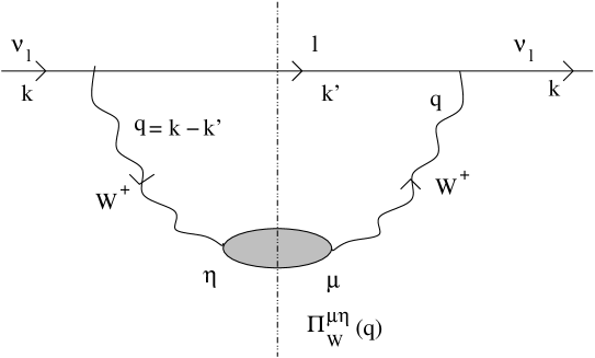
Figure 1: Diagrammatic representation of the neutrino selfenergy in nuclear matter.

$$\Sigma_{\nu}(k;\rho)=\frac{8{\rm i}G}{\sqrt{2}M^{2}_{W}}\int\frac{d^{4}q}{(2\pi)^{4}}\frac{L_{\eta\mu}\Pi^{\mu\eta}_{W}(q;\rho)}{k^{\prime 2}-m^{2}_{l}+{\rm i}\epsilon}$$ (12)

The neutrino disappears from the elastic flux, by inducing one particle-one hole (1p1h), 2p2h $\cdots$ excitations, $\Delta(1232)-$hole ($\Delta$h) excitations or creating pions, etc… at a rate given by

$$\Gamma(k;\rho)=-\frac{1}{k^{0}}{\rm Im}\Sigma_{\nu}(k;\rho)$$ (13)

We get the imaginary part of $\Sigma_{\nu}$ by using the Cutkosky’s rules. In this case we cut with a straight vertical line (see Fig. 1) the intermediate lepton state and those implied by the $W-$boson polarization (shaded region). Those states are then placed on shell by taking the imaginary part of the propagator, selfenergy, etc. Thus, we obtain for $k^{0}>0$

$${\rm Im}\Sigma_{\nu}(k)=\frac{8G}{\sqrt{2}M^{2}_{W}}\int\frac{d^{3}k^{\prime}}{(2\pi)^{3}}\frac{\Theta(q^{0})}{2E^{\prime}_{l}}~{}{\rm Im}\left\{\Pi^{\mu\eta}_{W}(q;\rho)L_{\eta\mu}\right\}$$ (14)

with $\Theta(...)$ the Heaviside function. Since $\Gamma dtdS$ provides a probability times a differential of area, which is a contribution to the $(\nu_{l},l)$ cross section, we have

$$d\sigma = \Gamma(k;\rho)dtdS=-\frac{1}{k^{0}}{\rm Im}\Sigma_{\nu}(k;\rho)dtdS=-\frac{1}{|\vec{k}|}{\rm Im}\Sigma_{\nu}(k;\rho)d^{3}r$$ (15)

and hence the nuclear cross section is given by

$$\sigma=-\frac{1}{|\vec{k}|}\int{\rm Im}\Sigma_{\nu}(k;\rho(r))d^{3}r$$ (16)

where we have substituted $\Sigma_{\nu}$ as a function of the nuclear density at each point of the nucleus and integrate over the whole nuclear volume. Hence, we assume the Local Density Approximation, (LDA) which, as shown in Ref. CO92 , is an excellent approximation for volume processes like the one studied here. Coming back to Eq. (14) we find

$$\frac{d^{2}\sigma_{\nu l}}{d\Omega(\hat{k^{\prime}})dk^{\prime 0}} = -\frac{|\vec{k}^{\prime}|}{|\vec{k}~{}|}\frac{G^{2}}{4\pi^{2}}\left(\frac{2\sqrt{2}}{g}\right)^{2}\int\frac{d^{\,3}r}{2\pi}\Big{\{}L_{\mu\eta}^{s}~{}{\rm Im}(\Pi_{W}^{\mu\eta}+\Pi_{W}^{\eta\mu})-L_{\mu\eta}^{a}~{}{\rm Re}(\Pi_{W}^{\mu\eta}-\Pi_{W}^{\eta\mu)}\Big{\}}\Theta(q^{0})$$ (17)

and then by comparing to Eq. (3), the hadronic tensor reads

$$W^{\mu\sigma}_{s} = -\Theta(q^{0})\left(\frac{2\sqrt{2}}{g}\right)^{2}\int\frac{d^{3}r}{2\pi}~{}{\rm Im}\left[\Pi_{W}^{\mu\sigma}+\Pi_{W}^{\sigma\mu}\right](q;\rho)$$ (18)

$$W^{\mu\sigma}_{a} = -\Theta(q^{0})\left(\frac{2\sqrt{2}}{g}\right)^{2}\int\frac{d^{3}r}{2\pi}~{}{\rm Re}\left[\Pi_{W}^{\mu\sigma}-\Pi_{W}^{\sigma\mu}\right](q;\rho)$$ (19)

As we see, the basic object is the selfenergy of the Gauge Boson ($W^{\pm}$) inside of the nuclear medium. Following the lines of Ref. GNO97 , we should perform a many body expansion, where the relevant gauge boson absorption modes would be systematically incorporated: absorption by one nucleon, or a pair of nucleons or even three nucleon mechanisms, real and virtual meson ($\pi$, $\rho$, $\cdots$) production, excitation of $\Delta$ of higher resonance degrees of freedom, etc. In addition, nuclear effects such as RPA or Short Range Correlations (SRC) should also be taken into account. Some of the $W-$absorption modes are depicted in Fig. 2.

Figure 2: Diagrammatic representation of some diagrams contributing to the $W^{+}-$selfenergy.

Up to this point the formalism is rather general and its applicability has not been restricted to the QE region. In this work we will focus on the QE contribution to the total cross section, and it will be analyzed in detail in the next section.

III QE contribution to $\Pi_{W}^{\mu\nu}(q;\rho)$

The virtual $W^{+}$ can be absorbed by one nucleon leading to the QE contribution of the nuclear response function. Such a contribution corresponds to a 1p1h nuclear excitation (first of the diagrams depicted in Fig. 2). To evaluate this selfenergy, the free nucleon propagator in the medium is required.

$$S(p\,;\rho)=(\hbox to0.0pt{\hbox to5.03125pt{\hfil/\hfil}\hss}p+M)G(p\,;\rho),\qquad G(p\,;\rho)=\left(\frac{1}{p^{2}-M^{2}+{\rm i}\epsilon}+\frac{2\pi{\rm i}}{2E(\vec{p}\,)}\delta(p^{0}-E(\vec{p}\,))\Theta(k_{F}-|\vec{p}~{}|)\right)$$ (20)

with the local Fermi momentum $k_{F}(r)=(3\pi^{2}\rho(r)/2)^{1/3}$, $M=940$ MeV the nucleon mass, and $E(\vec{p}\,)=\sqrt{M^{2}+\vec{p}^{\,2}}$. We will work on a non-symmetric nuclear matter with different Fermi sea levels for protons, $k_{F}^{p}$, than for neutrons, $k_{F}^{n}$ (equation above, but replacing $\rho/2$ by $\rho_{p}$ or $\rho_{n}$, with $\rho=\rho_{p}+\rho_{n}$). On the other hand, for the $W^{+}pn$ vertex we take

$$<p;\vec{p}^{~{}\prime}=\vec{p}+\vec{q}~{}|j^{\alpha}_{cc}(0)|n;\vec{p}~{}>=\bar{u}(\vec{p}{~{}^{\prime}})(V^{\alpha}-A^{\alpha})u(p)$$ (21)

with vector and axial nucleon currents given by

$$V^{\alpha}=2\cos\theta_{C}\times\left(F_{1}^{V}(q^{2})\gamma^{\alpha}+{\rm i}\mu_{V}\frac{F_{2}^{V}(q^{2})}{2M}\sigma^{\alpha\nu}q_{\nu}\right),\qquad A^{\alpha}=\cos\theta_{C}G_{A}(q^{2})\times\left(\gamma^{\alpha}\gamma_{5}+\frac{2M}{m_{\pi}^{2}-q^{2}}q^{\alpha}\gamma_{5}\right)$$ (22)

with $m_{\pi}=139.57$ MeV. Partially conserved axial current and invariance under G-parity have been assumed to relate the pseudoscalar form factor to the axial one and to discard a term of the form $(p^{\mu}+p^{\prime\mu})\gamma_{5}$ in the axial sector, respectively. Invariance under time reversal guarantees that all form factors are real. Besides, Due to isospin symmetry, the vector form factors are related to the electromagnetic ones

$$F_{1}^{V}(q^{2})=\frac{1}{2}\left(F_{1}^{p}(q^{2})-F_{1}^{n}(q^{2})\right),\qquad\mu_{V}F_{2}^{V}(q^{2})=\frac{1}{2}\left(\mu_{p}F_{2}^{p}(q^{2})-\mu_{n}F_{2}^{n}(q^{2})\right)$$ (24)

and for the axial form-factor we use

$$G_{A}(q^{2})=\frac{g_{A}}{(1-q^{2}/M_{A}^{2})^{2}},\quad g_{A}=1.257,\quad M_{A}=1.049~{}{\rm GeV}$$ (25)

With all of these ingredients is straightforward to evaluate the contribution to the $W^{+}-$selfenergy of the first diagram of Fig. 2,

$$-{\rm i}\Pi_{W}^{\mu\nu}(q^{0},\vec{q}\,)=-\cos^{2}\theta_{C}\left(\frac{g}{2\sqrt{2}}\right)^{2}\int\frac{d^{4}p}{(2\pi)^{4}}A^{\mu\nu}(p,q)G(p;\rho_{n})G(p+q;\rho_{p})$$ (26)

with the CC nucleon tensor given by

$$A^{\mu\nu}(p,q) = Tr\left\{\left(2F_{1}^{V}\gamma^{\mu}-2{\rm i}\mu_{V}\frac{F_{2}^{V}}{2M}\sigma^{\mu\alpha}q_{\alpha}-G_{A}\left(\gamma^{\mu}\gamma_{5}-\frac{2M}{m_{\pi}^{2}-q^{2}}q^{\mu}\gamma_{5}\right)\right)(\hbox to0.0pt{\hbox to5.03125pt{\hfil/\hfil}\hss}p+\hbox to0.0pt{\hbox to5.00002pt{\hfil$q$\hfil}\hss}/+M)\right.$$ (27)

$$\times \left.\left(2F_{1}^{V}\gamma^{\nu}+2{\rm i}\mu_{V}\frac{F_{2}^{V}}{2M}\sigma^{\nu\beta}q_{\beta}-G_{A}\left(\gamma^{\nu}\gamma_{5}+\frac{2M}{m_{\pi}^{2}-q^{2}}q^{\nu}\gamma_{5}\right)\right)(\hbox to0.0pt{\hbox to5.03125pt{\hfil/\hfil}\hss}p+M)\right\}$$

The Dirac’s space traces above can be easily done and the nucleon tensor can be found in Sect. A.1 of the Appendix. Subtracting the divergent vacuum contribution in Eq. (26), we finally get from Eqs. (18) and  (19)

$$W^{\mu\nu}(q^{0},\vec{q}\,) = -\frac{\cos^{2}\theta_{C}}{2M^{2}}\int_{0}^{\infty}drr^{2}\Big{\{}2\Theta(q^{0})\int\frac{d^{3}p}{(2\pi)^{3}}\frac{M}{E(\vec{p})}\frac{M}{E(\vec{p}+\vec{q})}\Theta(k_{F}^{n}(r)-|\vec{p}~{}|)\Theta(|\vec{p}+\vec{q}~{}|-k_{F}^{p}(r))$$ (28)

$$\times (-\pi)\delta(q^{0}+E(\vec{p})-E(\vec{p}+\vec{q}~{}))A^{\nu\mu}(p,q)|_{p^{0}=E(\vec{p})~{}}\Big{\}}$$

The $d^{3}p$ integrations above can be analytically done and all of them are determined by the imaginary part of the relativistic isospin asymmetric Lindhard function, $\overline{U}_{R}(q,k_{F}^{n},k_{F}^{p})$. Explicit expressions can be found in Sect. B of the Appendix.

Up to this point the treatment is fully relativistic and the four momentum transferred to the nucleus can be comparable or higher than the nucleon mass. At low and intermediate energies, RPA effects become extremely large, as shown for instance in Ref Ch90 . To account for RPA effects, we will use a nucleon–nucleon effective force Sp77 determined from calculations of nuclear electric and magnetic moments, transition probabilities and giant electric and magnetic multipole resonances using a non-relativistic nuclear dynamics scheme. This force, supplemented by nucleon–$\Delta(1232)$ and $\Delta(1232)$–$\Delta(1232)$ interactions OTW82 -pion , was successfully used in the work of Ref. GNO97 on inclusive nuclear electron scattering. In this latter reference a non-relativistic LFG is also employed. Thus, it is of interest to discuss also the hadronic tensor of Eq. (28) in the context of a non-relativistic Fermi gas. This is easily done by replacing the factors $M/E(\vec{p})$ and $M/E(\vec{p}+\vec{q})$ in Eq. (28) by one. Explicit expressions can be now found in Sect. C of the Appendix.

Pauli blocking, through the imaginary part of the Lindhard function, is the main nuclear effect included in the hadronic tensor of Eq. (28). In the next subsections, we will study different nuclear corrections to $W^{\mu\nu}$.

To finish this section, we devote a few words to the Low Density Theorem (LDT). At low nuclear densities the imaginary part of the relativistic isospin asymmetric Lindhard function can be approximated by

$${\rm Im}\overline{U}_{R}(q,k_{F}^{n},k_{F}^{p})\approx-\pi\rho_{n}\frac{M}{E(\vec{q}\,)}\delta(q^{0}+M-E(\vec{q}\,))$$ (29)

and thus one readily finds

$$\sigma_{\nu_{l}+\,A_{Z}\to l^{-}+X}\approx N\sigma_{\nu_{l}+\,n\to l^{-}+p},\qquad N=A-Z$$ (31)

which accomplishes with the LDT. For future purposes we give in Sect. D of the Appendix the $\nu_{l}+\,n\to l^{-}+p$ differential cross section.

III.1 RPA Nuclear Correlations

When the electroweak interactions take place in nuclei, the strengths of electroweak couplings may change from their free nucleon values due to the presence of strongly interacting nucleons Ch90 . Indeed, since the nuclear experiments on $\beta$ decay in the early seventies Wi74 , the quenching of axial current is a well established phenomenon. We follow here the MBF of Ref. GNO97 , and take into account the medium polarization effects in the 1p1h contribution to the $W-$selfenergy by substituting it by an RPA response as shown diagrammatically in Fig. 3. For that purpose we use an effective ph–ph interaction of the Landau-Migdal type

$$\begin{array}[]{ll}V=&c_{0}\Big{\{}f_{0}(\rho)+f_{0}^{\prime}(\rho)\vec{\tau}_{1}\vec{\tau}_{2}+g_{0}(\rho)\vec{\sigma}_{1}\vec{\sigma}_{2}+g_{0}^{\prime}(\rho)\vec{\sigma}_{1}\vec{\sigma}_{2}\vec{\tau}_{1}\vec{\tau}_{2}\Big{\}}\end{array}$$ (32)

where $\vec{\sigma}$ and $\vec{\tau}$ are Pauli matrices acting on the nucleon spin and isospin spaces, respectively. Note that the above interaction is of contact type, and therefore in coordinate space one has $V(\vec{r}_{1},\vec{r}_{2})\propto\delta(\vec{r}_{1}-\vec{r}_{2})$. As mentioned before, the coefficients were determined in Ref. Sp77 from calculations of nuclear electric and magnetic moments, transition probabilities, and giant electric and magnetic multipole resonances. They are parameterized as

$$f_{i}(\rho(r))=\frac{\rho(r)}{\rho(0)}f_{i}^{(in)}+\left[1-\frac{\rho(r)}{\rho(0)}\right]f_{i}^{(ex)}$$ (33)

where

$$\begin{array}[]{ll}f_{0}^{(in)}=0.07&f_{0}^{\prime(ex)}=0.45\\ f_{0}^{(ex)}=-2.15&f_{0}^{\prime(in)}=0.33\\ g_{0}^{(in)}=g_{0}^{(ex)}=g_{0}=0.575{}{}{}{}{}{}{}{}{}&g_{0}^{\prime(in)}=g_{0}^{\prime(ex)}=g_{0}^{\prime}=0.725\\ \end{array}$$ (34)

and $c_{0}=380\,{\rm MeVfm}^{3}$. In the $S=1=T$ channel ($\vec{\sigma}\vec{\sigma}\vec{\tau}\vec{\tau}$ operator) we use an interaction with explicit $\pi$ (longitudinal) and $\rho$ (transverse) exchanges, which has been used for the renormalization of the pionic and pion related channels in different nuclear reactions at intermediate energies GNO97 , CO92 –pion . Thus we replace,

$$c_{0}g_{0}^{\prime}(\rho)\vec{\sigma}_{1}\vec{\sigma}_{2}\vec{\tau}_{1}\vec{\tau}_{2}\to\vec{\tau}_{1}\vec{\tau}_{2}\sum_{i,j=1}^{3}\sigma_{1}^{i}\sigma_{2}^{j}V_{ij}^{\sigma\tau},\qquad V_{ij}^{\sigma\tau}=\left(\hat{q}_{i}\hat{q}_{j}V_{l}(q)+({\delta}_{ij}-\hat{q}_{i}\hat{q}_{j})V_{t}(q)\right)$$ (35)

with $\hat{q}=\vec{q}/|\vec{q}\,|$ and the strengths of the ph-ph interaction in the longitudinal and transverse channel are given by

$$V_{l}(q^{0},\vec{q}) = \frac{f^{2}}{m^{2}_{\pi}}\left\{\left(\frac{\Lambda_{\pi}^{2}-m_{\pi}^{2}}{\Lambda_{\pi}^{2}-q^{2}}\right)^{2}\frac{\vec{q}{\,{}^{2}}}{q^{2}-m_{\pi}^{2}}+g^{\prime}_{l}(q)\right\},\qquad\frac{f^{2}}{4\pi}=0.08,~{}~{}\Lambda_{\pi}=1200~{}{\rm MeV}$$

$$V_{t}(q^{0},\vec{q}) = \frac{f^{2}}{m^{2}_{\pi}}\left\{C_{\rho}\left(\frac{\Lambda_{\rho}^{2}-m_{\rho}^{2}}{\Lambda_{\rho}^{2}-q^{2}}\right)^{2}\frac{\vec{q}{\,{}^{2}}}{q^{2}-m_{\rho}^{2}}+g^{\prime}_{t}(q)\right\},\qquad C_{\rho}=2,~{}~{}\Lambda_{\rho}=2500~{}{\rm MeV},~{}~{}m_{\rho}=770~{}{\rm MeV}$$ (36)

Figure 3: Set of irreducible diagrams responsible for the polarization (RPA) effects in the 1p1h contribution to the $W-$selfenergy.

The SRC functions $g^{\prime}_{l}$ and $g^{\prime}_{t}$ have a smooth $q-$dependence OTW82 ; Ga88 , which we will not consider here, and thus we will take $g^{\prime}_{l}(q)=g^{\prime}_{t}(q)=g^{\prime}=0.63$ as it was done in the study of inclusive nuclear electron scattering carried out in Ref. GNO97 , and also in some of the works of Ref. pion . Note that, $c_{0}g^{\prime}_{0}$ and $g^{\prime}f^{2}/m_{\pi}^{2}$ differ from each other in less than 10%.

We also include $\Delta(1232)$ degrees of freedom in the nuclear medium which, given the spin-isospin quantum numbers of the $\Delta$ resonance, only modify the vector-isovector ($S=1=T$) channel of the RPA response function. The ph–$\Delta$h and $\Delta$h–$\Delta$h effective interactions are obtained from Eqs. (35) and (36) by replacing $\vec{\sigma}\to\vec{S}$, $\vec{\tau}\to\vec{T}$, where $\vec{S},\vec{T}$ are the spin, isospin $N\Delta$ transition operators OTW82 and $f\to f^{*}=2.13~{}f$, for any $\Delta$ which replaces a nucleon.

Thus, the $V$ lines in Fig. 3 stand for the effective ph($\Delta$h)-ph($\Delta$h) interaction described so far. Given the isospin structure of the $W^{\pm}NN$ coupling, the isoscalar terms ($f_{0}$ and $g_{0}$) of the effective interaction can not contribute to the RPA response function. We should stress that this effective interaction is non-relativistic, and then for consistency we will neglect terms of order ${\cal O}(p^{2}/M^{2})$ when summing up the RPA series.

To start with, let us examine how the axial vector term ($G_{A}\gamma^{\mu}\gamma_{5}\tau_{+}/2$, where $\tau_{\pm}=\tau_{x}\pm{\rm i}\tau_{y}$ are the ladder isospin operators responsible for the $n$ to $p$ and $p$ to $n$ transitions, $\tau^{+}|n>=2|p>$) of the CC axial current is renormalized. As mentioned above, we will only compute the higher density corrections, implicit in the RPA series, to the leading and next-to-leading orders in the $p/M$ expansion. The nonrelativistic reduction of the axial vector term in the nucleon current reads

$$G_{A}\overline{u}_{r^{\prime}}(\vec{p}^{\,\prime})\frac{\tau_{+}}{2}\gamma^{\mu}\gamma_{5}u_{r}(p)=2MG_{A}\chi^{\dagger}_{r^{\prime}}\left(-g^{\mu i}\sigma^{i}+g^{\mu 0}\frac{\vec{\sigma}\cdot(\vec{p}+\vec{p}^{\,\prime})}{2M}+\cdots\right)\frac{\tau_{+}}{2}\chi_{r},\quad i=1,2,3$$ (37)

with $\vec{p}^{\,\prime}=\vec{p}+\vec{q}$, and $\chi_{r}$ a non-relativistic nucleon spin-isospin wave-function. In Eq. (37) there is a sum on the repeated index $i$ and the dots stand for corrections of order ${\cal O}\left(\vec{p}^{\,2}/M^{2},\vec{p}^{\,\prime 2}/M^{2},q^{0}/M\right)$. In the impulse approximation, this current leads to a CC nucleon tensor,

$$A^{\mu\nu}(p,q)|_{{\rm axial~{}vector}}^{NR}=8M^{2}\left({\cal A}_{1}^{\mu\nu}+{\cal A}_{2}^{\mu\nu}\right),\quad{\cal A}_{1}^{\mu\nu}=G_{A}^{2}g^{\mu i}g^{\nu j}\delta^{ij},\quad{\cal A}_{2}^{\mu\nu}=-G_{A}^{2}\left(g^{\mu i}g^{\nu 0}+g^{\mu 0}g^{\nu i}\right)\frac{(2\vec{p}+\vec{q}\,)^{i}}{2M}$$ (38)

with $i,j=1,2,3$ and there is again a sum for repeated indices. The tensor $A^{\mu\nu}(p,q)|_{{\rm axial~{}vector}}^{NR}$ can be also obtained from the non-relativistic reduction of $A^{\mu\nu}(p,q)$ in Eq. (66). The ${\cal A}_{1}$ contribution comes from the leading operator $-g^{\mu i}\sigma^{i}\tau_{+}/2$, and involves the trace of $G_{A}^{2}\sigma^{i}\sigma^{j}$ (1p1h excitation depicted in the first diagram of Fig. 3). Let us consider first this simple operator and only forward propagating (direct term of the Lindhard function) ph–excitations. Taking into account the spin structure of this operator the scalar term $f_{0}^{\prime}$ of the effective interaction does not contribute either, and thus we are left with the spin-isospin channel of the effective interaction, $\sum_{ij}V_{ij}^{\sigma\tau}\sigma_{1}^{i}\sigma_{2}^{j}\vec{\tau}_{1}\vec{\tau}_{2}$. Let us now look at the irreducible diagrams consisting of the excitation of one and two ph states (first and second diagrams of Fig. 3). The contribution of those diagrams to the W-selfenergy is

$$\Pi^{ij}_{W} \propto ~{}<p|\frac{\tau_{+}}{2}|n><n|\frac{\tau_{-}}{2}|p>\frac{\overline{U}}{2}Tr(\sigma^{i}\sigma^{j})$$ (39)

$$+ <p|\frac{\tau_{+}}{2}|n><n|\vec{\tau}|p><p|\vec{\tau}|n><n|\frac{\tau_{-}}{2}|p>\left(\frac{\overline{U}}{2}\right)^{2}\sum_{k,l=1}^{3}Tr(\sigma^{i}\sigma^{l})Tr(\sigma^{k}\sigma^{j})V^{\sigma\tau}_{lk}$$

$$= \overline{U}(q,k_{F}^{n},k_{F}^{p})\left(\delta^{ij}+2\overline{U}(q,k_{F}^{n},k_{F}^{p})V^{ij}_{\sigma\tau}\right)$$

The excitation of three ph states gives a contribution of $\overline{U}(2\overline{U})^{2}\sum_{k}V^{ik}_{\sigma\tau}V^{kj}_{\sigma\tau}=\overline{U}(2\overline{U})^{2}\left(\hat{q}_{i}\hat{q}_{j}V_{l}^{2}+({\delta}_{ij}-\hat{q}_{i}\hat{q}_{j})V_{t}^{2}\right)$ to $\Pi^{ij}_{W}$. Thus, the full sum of multiple ph excitation states, implicit in Fig. 3, leads to two independent geometric series, in the longitudinal and transverse channels, which are taken into account by the following substitution in the hadronic tensor ($W^{\mu\nu}$)

$$\delta^{ij}8M^{2}G_{A}^{2}{\rm Im}\overline{U}(q,k_{F}^{n},k_{F}^{p}) \to 8M^{2}G_{A}^{2}{\rm Im}\left\{\overline{U}(q,k_{F}^{n},k_{F}^{p})\left(\frac{\hat{q}^{i}\hat{q}^{j}}{1-2\overline{U}(q,k_{F}^{n},k_{F}^{p})V_{l}(q)}+\frac{\delta^{ij}-\hat{q}^{i}\hat{q}^{j}}{1-2\overline{U}(q,k_{F}^{n},k_{F}^{p})V_{t}(q)}\right)\right\}$$ (40)

$$= 8M^{2}G_{A}^{2}{\rm Im}\overline{U}(q,k_{F}^{n},k_{F}^{p})\left(\frac{\hat{q}^{i}\hat{q}^{j}}{|1-2\overline{U}(q,k_{F}^{n},k_{F}^{p})V_{l}(q)|^{2}}+\frac{\delta^{ij}-\hat{q}^{i}\hat{q}^{j}}{|1-2\overline{U}(q,k_{F}^{n},k_{F}^{p})V_{t}(q)|^{2}}\right)$$

The factor 2 in the denominator above and that in Eq. (39) comes from the isospin dependence, $\vec{\tau}_{1}\cdot\vec{\tau}_{2}$, of the effective ph–ph interaction. Taking account of $\Delta$h and backward (crossed term of the Lindhard function) propagating ph excitations (see Fig. 3), not accounted for by $\overline{U}$ is readily done by substituting $2\overline{U}$ in the denominator by $U(q,k_{F})=U_{N}+U_{\Delta}$, the Lindhard function of Ref. Ga88 , which for simplicity we evaluate in an isospin symmetric nuclear medium of density $\rho$. The different couplings for $N$ and $\Delta$ are incorporated in $U_{N}$ and $U_{\Delta}$ and then the same interaction strengths $V_{l}$ and $V_{t}$ are used for ph and $\Delta$h excitations OTW82 ; pion . Taking $\vec{q}$ in the $z$ direction, Eq. (40) implies that the axial vector contribution to the transverse ($xx,yy$) and longitudinal ($zz$) components of the hadronic tensor get renormalized by different factors $1/|1-U(q,k_{F})V_{t}(q)|^{2}$ versus $1/|1-U(q,k_{F})V_{l}(q)|^{2}$.

Let us pay now attention to the term ${\cal A}_{2}$ in Eq. (38), it comes from the interference between the $-g^{\mu i}\sigma^{i}\tau_{+}/2$ and $\tau_{+}g^{\mu 0}\left(\vec{\sigma}\cdot(\vec{p}+\vec{p}^{\,\prime})\right)/4M$ operators in Eq. (37). The consideration of the full RPA series leads now to the substitution

$$8M^{2}\frac{q^{0}}{|\vec{q}\,|}G^{2}_{A}{\rm Im}\overline{U}(q,k_{F}^{n},k_{F}^{p})\to 8M^{2}\frac{q^{0}}{|\vec{q}\,|}G^{2}_{A}\frac{{\rm Im}\overline{U}(q,k_{F}^{n},k_{F}^{p})}{|1-U(q,k_{F})V_{l}(q)|^{2}}$$ (41)

in the $0z$ and $z0$ components of the hadronic tensor $W^{\mu\nu}$.

Keeping track of the responsible operators, we have examined and renormalized all different contributions to the CC nucleon tensor $A^{\mu\nu}$, by summing up the RPA series depicted in Fig. 3. The $00,0z,zz,xx$ and $xy$ components of the RPA renormalized CC nucleon tensor can be found in Sect. A.2 of the Appendix. As mentioned above, since the ph($\Delta$h)-ph($\Delta$h) effective interaction is non-relativistic, we have computed polarization effects only for the leading and next-to-leading terms in the $p/M$ expansion. Thus, order ${\cal O}\left(k_{F}\vec{p}^{\,2}/M^{2},k_{F}\vec{p}^{\,\prime 2}/M^{2},k_{F}q^{0}/M\right)$ has been neglected in the formulae of the Sect. A.2 of the Appendix. We have made an exception to the above rule, and since $\mu_{V}$ could be relatively large, we have taken $\mu_{V}F_{2}^{V}|\vec{q}\,|/M$ to be of order ${\cal O}(0)$ in the $p/M$ expansion. Finally, we should stress that the scalar–isovector term of the effective interaction ($f^{\prime}$) cannot produce $\Delta$h excitations and therefore, when this term is involved in the RPA renormalization, only the nucleon Lindhard function ($U_{N}$) appears (see coefficient ${\bf C_{N}}$ in Eq. (74)).

To finish this subsection we will discuss the differences between the medium polarization scheme presented here and that undertaken in Refs. Ch90 ; Si92 . There is an obvious difference, since in these latter references the scalar-isovector term ($f^{\prime}$) of the ph–ph effective interaction was not taken into account. In addition, there are some differences concerning the tensorial treatment of the RPA response function. In the framework presented in this work we firstly evaluate the 1p1h hadronic tensor and all sort of polarization (RPA) corrections to the different components of this tensor. In a second step we contract it with the leptonic tensor and obtain the differential cross section. The RPA corrections do not depend only on the different terms of the nucleon currents, but also on the particular component of the hadronic tensor which is being renormalized. Thus, as it is obvious, the RPA corrections, in general, are different for each of the terms ($(F_{1}^{V})^{2},(F_{2}^{V})^{2},F_{1}^{V}F_{2}^{V},G_{A}^{2},G_{P}^{2},G_{A}G_{P},F_{1}^{V}G_{A}$ and $F_{2}^{V}G_{A}$, with $G_{P}=2MG_{A}/(m^{2}_{\pi}-q^{2})$ ) appearing in the CC nucleon tensor. Besides, for a fixed term, the polarization effects do also depend on the tensor component. Indeed, we have already mentioned this fact in the discussion of Eq. (40), where we saw that the axial vector contribution to the transverse ($xx$,$yy$) and the longitudinal ($zz$) components of the hadronic tensor get renormalized by different factors.

In the works of Refs. Ch90 ; Si92 the 1p1h hadronic tensor, without polarization effects included, is first contracted with the leptonic one. This contraction is denoted as, up to global kinematical factors, $\overline{\sum}\sum|T|^{2}$ in those references. In a second step, the authors of Refs. Ch90 ; Si92 study the medium polarization corrections to $\overline{\sum}\sum|T|^{2}$. They find out different medium corrections for each of the terms of the CC nucleon tensor ($(F_{1}^{V})^{2},\cdots,F_{2}^{V}G_{A}$), as we do. However, for a fixed term, they cannot independently study the effect of the RPA re-summation in each of the different tensor components, since they are not dealing with the hadronic tensor itself, but with the contraction of it with the leptonic one. As a matter of example, to account for the RPA corrections to the axial vector–axial vector term, the following substitution is given in Refs. Ch90 ; Si92

$$G_{A}^{2}\to G_{A}^{2}\left(\frac{2}{3|1-U(q,k_{F})V_{t}(q)|^{2}}+\frac{1}{3|1-U(q,k_{F})V_{l}(q)|^{2}}\right)$$ (42)

The above substitution can be recovered from Eq. (40) by contracting this latter equation with $\delta_{ij}$, and replacing $2\overline{U}\to U$. Thus, Eq. (42) is strictly correct, neglecting terms of order $p/M$, only for the contribution to $\overline{\sum}\sum|T|^{2}$ obtained from the contraction of the hadronic tensor with the $g_{\mu\nu}$ term of the leptonic one. The prescription of Eq. (42) is not correct for those contributions to $\overline{\sum}\sum|T|^{2}$ arising from the contraction of the $k^{\prime}_{\mu}k_{\sigma}+k^{\prime}_{\sigma}k_{\mu}$ terms of the leptonic tensor with the axial vector–axial vector contribution of $W^{\mu\nu}$. Note however that neglecting the bound muon three momentum and up to terms of order $p/M$, Eq. (42) is correct for the study of inclusive muon capture in nuclei, where it was first used by the authors of Refs. Ch90 ; Si92 , and it is also reasonable for neutrino–nucleus reactions at low energies, where the RPA effects are more important.

III.2 Correct Energy Balance and Coulomb Distortion Effects

To ensure the correct energy balance in the reaction (2) for finite nuclei, the energy conserving $\delta$ function in Eq. (28) has to be modified Ch90 ; Si92 . The energies $E(\vec{p})$ and $E(\vec{p}+\vec{q}~{})$ in the argument of the $\delta$ function refer to the LFG of the nucleons in the initial and final nucleus. In the Fermi sea there is no energy gap for the transition from the occupied to the unoccupied states and hence ph excitations can be produced with a small energy, $Q^{\rm LFG}(r)=E_{F}^{p}(r)-E_{F}^{n}(r)$ . However, in actual nuclei there is a minimum excitation energy, $Q=M(A_{Z+1})-M(A_{Z})$, needed for the transition to the ground state of the final nucleus. For instance , this $Q$ value is 16.827 MeV for the transition ${}^{12}{\rm C}_{gs}\to^{12}{\rm N}_{gs}$ and the consideration of this energy gap is essential to obtain reasonable cross sections for low-energy neutrinos. We have taken it into account by replacing

$$q^{0}\to q^{0}-(Q-Q^{\rm LFG}(r))$$ (43)

in the $\delta-$function of the right hand side of Eq. (28).

The second effect which we want to address here is due to the fact that the charged lepton produced in the reaction of Eq. (2) is moving in the Coulomb field of the nucleus described by a charge distribution $\rho_{ch}(r)$. In our scheme, we implement the corrections due to this effect following the semiclassical approximation used in Ref. Si92 . Thus, we include a selfenergy (Coulomb potential) in the intermediate lepton propagator of the neutrino selfenergy depicted in Fig. 1. We approximate this selfenergy inside the LFG by

$$\Sigma_{C}=2k^{\prime 0}V_{C}(r),\quad V_{C}(r)=-4\pi\alpha\left(\frac{1}{r}\int_{0}^{r}dr^{\prime}r^{\prime 2}\rho_{ch}(r^{\prime})+\int_{r}^{+\infty}dr^{\prime}r^{\prime}\rho_{ch}(r^{\prime})\right)$$ (44)

with $\alpha=1/137.036$ and the charge distribution, $\rho_{ch}$, normalized to $Z$. The evaluation of the imaginary part of the $\nu$ self-energy in the medium requires to put the intermediate lepton propagator on the mass shell. Following the Cutkosky’s rules, and neglecting quadratic corrections in $V_{C}$, we find

$$\frac{1}{k^{\prime\,2}-m^{2}_{l}-2k^{\prime 0}V_{C}(r)+{\rm i}\epsilon}\to-{\rm i}\pi\frac{\delta(k^{\prime 0}-E^{\prime}_{l})}{k^{\prime 0}}\Theta(\hat{E}^{\prime}_{l}(r)-m_{l})$$ (45)

where $E^{\prime}_{l}$ is the asymptotical outgoing lepton energy in regions where the Coulomb potential can be neglected, and the local outgoing lepton energy, $\hat{E}^{\prime}_{l}(r)$, is defined by energy conservation

$$\hat{E}^{\prime}_{l}(r)+V_{C}(r)=\sqrt{m_{l}^{2}+\vec{{\cal K}}^{\,\prime 2}(r)}+V_{C}(r)=E^{\prime}_{l}$$ (46)

Because of the Coulomb potential, the outgoing lepton three momentum, $\vec{{\cal K}}^{\,\prime}$, is not longer conserved, and it becomes a function of $r$, taking its asymptotical value, $\vec{k}^{\,\prime}$, at large distances. Therefore, $\vec{q}$ should also be replaced by a local function: $\vec{q}^{\,\,\prime}(r)=\vec{k}-\vec{{\cal K}}^{\,\prime}(r)$. Furthermore, from the $d^{3}k^{\prime}$ integration in Eq. (14), and considering now the locality of the three momentum, we get from phase space a correction factor $|\vec{{\cal K}}^{\,\prime}(r)|\hat{E}^{\prime}_{l}(r)/|\vec{k}^{\,\prime}|E^{\prime}_{l}$. This way of taking into account the Coulomb effects has clear resemblances with what is called “modified effective momentum approximation” in Ref. En98 . The use of a plane-wave approximation in the interaction region is equivalent to the assumption that the Coulomb potential does not change the direction of the particles when they leave the nucleus. It should therefore not strongly alter an outgoing negatively charged lepton wave packet, which asymptotically is spherical, after it leaves the nucleus except by slowing it down and thereby changing the average radial wavelength and amplitude as the wave moves to larger $r$. As it is shown in En98 , for total cross sections this procedure works very accurately for muons down to low energies. For low- energy electrons and positrons it is less accurate, and the use of the Fermi function $F(Z,E^{\prime}_{l})$ (Be82 ) is widely accepted in the literature. Anyway, Coulomb effects are small and they become relatively sizeable only for neutrino induced reactions near threshold and/or for heavy nuclei.

To summarize the results of Subsections III.1 and III.2, our final expression for the hadronic tensor is given by

$$W^{\mu\nu}(q^{0},\vec{q}\,) = -\frac{\cos^{2}\theta_{C}}{2M^{2}}\int_{0}^{\infty}drr^{2}\frac{|\vec{{\cal K}}^{\,\prime}(r)|\hat{E}^{\prime}_{l}(r)}{|\vec{k}^{\,\prime}|E^{\prime}_{l}}\Theta(\hat{E}^{\prime}_{l}(r)-m_{l})\Big{\{}2\Theta(q^{\prime 0})\int\frac{d^{3}p}{(2\pi)^{3}}\frac{M}{E(\vec{p})}\frac{M}{E(\vec{p}+\vec{q}^{\,\,\prime})}\times$$ (47)

$$\Theta(k_{F}^{n}(r)-|\vec{p}~{}|)\Theta(|\vec{p}+\vec{q}^{\,\,\prime}\,|-k_{F}^{p}(r))(-\pi)\delta\left(q^{\prime\,0}+E(\vec{p})-E(\vec{p}+\vec{q}^{\,\,\prime}\,)\right)A^{\nu\mu}_{\rm RPA}(p,q^{\prime})|_{p^{0}=E(\vec{p})~{}}\Big{\}}$$

with $q^{\prime 0}=q^{0}-(Q-Q^{\rm LFG}(r))$, $\vec{q}^{\,\,\prime}(r)=\vec{k}-\vec{{\cal K}}^{\,\prime}(r)$, and $A^{\mu\nu}_{\rm RPA}$ given in Sect. A.2 of the Appendix.

III.3 FSI Effects

Once a ph excitation is produced by the virtual $W-$boson, the outgoing nucleon can collide many times, thus inducing the emission of other nucleons. The result of it is a quenching of the QE peak respect to the simple ph excitation calculation and a spreading of the strength, or widening of the peak. The integrated strength over energies is not much affected though. A distorted wave approximation with an optical (complex) nucleon nucleus potential would remove all these events. However, if we want to evaluate the inclusive $(\nu_{l},l^{-})$ cross section these events should be kept and one must sum over all open final state channels.

In our MBF we will account for the FSI by using nucleon propagators properly dressed with a realistic selfenergy in the medium, which depends explicitly on the energy and the momentum FO92 . This selfenergy leads to nucleon spectral functions in good agreement with accurate microscopic approaches like the ones of Refs. Ra89 ; Mu95 . The selfenergy of Ref. FO92 has a proper energy–momentum dependence plus an imaginary part from the coupling to the 2p2h components, which is equivalent to the use of correlated wave functions, evaluated from realistic $NN$ forces and incorporating the effects of the nucleon force in the nucleon pairs. Thus, we consider the many body diagram depicted in Fig. 4 (there the dashed lines stand for an $NN$ interaction inside of the nuclear medium OTW82 ; FO92 ).

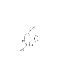
Figure 4: $W^{+}-$selfenergy diagram obtained from the first diagram depicted in Fig. 2 by dressing up the nucleon propagator of the particle state in the ph excitation.

However, a word of caution is in order since the imaginary part of this diagram presents a divergency. The reason is that when placing the 2p2h excitation on the mass shell through Cutkosky rules, we still have the square of the nucleon propagator with momentum $p+q$ in the figure. This propagator can be placed on shell for virtual $W-$bosons and we get a divergence.

Figure 5: Insertion of the nucleon selfenergy on the nucleon line of the particle state.

The divergence is not spurious, in the sense that its meaning is the probability per unit time of absorbing a virtual $W^{+}$ by one nucleon times the probability of collision of the final nucleon with other nucleons in the infinite Fermi sea in the lifetime of this nucleon. Since this nucleon is real, its lifetime is infinite and thus the probability is infinite, as well. The problem is physically solved Sa88 by recalling that the nucleon in the Fermi sea has a selfenergy with an imaginary part which gives it a finite lifetime (for collisions). This is taken into account by iterating, in the Dyson equation sense, the nucleon selfenergy insertion of Fig. 5 in the nucleon line, hence substituting the particle nucleon propagator, $G(p;\rho)$, in Eq. (20) by a renormalized nucleon propagator, $G_{\rm FSI}(p;\rho)$, including the nucleon selfenergy in the medium, $\Sigma(p^{0},\vec{p}\,;\rho)$,

$$G_{\rm FSI}(p;\rho)=\frac{1}{p^{0}-{\bar{E}}(\vec{p}\,)-\Sigma(p^{0},\vec{p}\,;\rho)}$$ (48)

with ${\bar{E}}(\vec{p}\,)=M+\vec{p}^{\,2}/2M$. As mentioned above, we use here the nucleon selfenergy model developed in Ref. FO92 , which led to excellent results in the study of inclusive electron scattering from nuclei GNO97 . Since the model of Ref. FO92 is not Lorentz relativistic and it also considers an isospin symmetric nuclear medium, we will only discuss the FSI effects for nuclei with approximately equal number of protons and neutrons, and using non-relativistic kinematics for the nucleons (see Sect. C of the Appendix). Thus, we have obtained Eq. (48) from the non-relativistic reduction of $G(p;\rho)$, in Eq. (20), by including the nucleon selfenergy.

Alternatively to the nucleon selfenergy language, one can use the spectral function representation

$$G_{\rm FSI}(p;\rho)=\int_{-\infty}^{\mu}\frac{S_{h}(\omega,\vec{p}\,;\rho)}{p^{0}-\omega-i\epsilon}d\omega+\int_{\mu}^{\infty}\frac{S_{p}(\omega,\vec{p}\,;\rho)}{p^{0}-\omega+i\epsilon}d\omega$$ (49)

where $S_{h},S_{p}$ are the hole and particle spectral functions related to nucleon selfenergy $\Sigma$ by means of

$$S_{p,h}(\omega,\vec{p}\,;\rho) = \mp\frac{1}{\pi}\frac{{\rm Im}\Sigma(\omega,\vec{p}\,;\rho)}{\Big{[}\omega-{\bar{E}}(\vec{p}\,)-{\rm Re}\Sigma(\omega,\vec{p}\,;\rho)\Big{]}^{2}+\Big{[}{\rm Im}\Sigma(\omega,\vec{p}\,;\rho)\Big{]}^{2}}$$ (50)

with $\omega\geq\mu$ or $\omega\leq\mu$ for $S_{p}$ and $S_{h}$, respectively. The chemical potential $\mu$ is determined by

$$\mu=M+\frac{k_{F}^{2}}{2M}+{\rm Re}\Sigma(\mu,k_{F})$$ (51)

By means of Eq. (49) we can write the ph propagator or new Lindhard function incorporating the effects of the nucleon selfenergy in the medium, and we have for its imaginary part (for positive values of $q^{0}$)

$${\rm Im}\overline{U}_{FSI}(q;k_{F})=-\frac{\Theta(q^{0})}{4\pi^{2}}\int d^{3}p\int_{\mu-q^{0}}^{\mu}d\omega S_{h}(\omega,\vec{p}\,;\rho)S_{p}(q^{0}+\omega,\vec{p}+\vec{q}\,;\rho)$$ (52)

Comparing the above expression with that of the ordinary imaginary part of the non-relativistic Lindhard function, Eq. (88), one realizes that to account for FSI effects in an isospin symmetric nuclear medium of density $\rho$ we should make the following substitution

$$2\Theta(q^{0})\int\frac{d^{3}p}{(2\pi)^{3}}\Theta(k_{F}^{n}(r)-|\vec{p}~{}|)\Theta(|\vec{p}+\vec{q}~{}|-k_{F}^{p}(r))(-\pi)\delta(q^{0}+{\bar{E}}(\vec{p})-{\bar{E}}(\vec{p}+\vec{q}~{}))A^{\nu\mu}(p,q)|_{p^{0}={\bar{E}}(\vec{p})~{}}$$ (53)

$$\rightarrow -\frac{\Theta(q^{0})}{4\pi^{2}}\int d^{3}p\int_{\mu-q^{0}}^{\mu}d\omega S_{h}(\omega,\vec{p}\,;\rho)S_{p}(q^{0}+\omega,\vec{p}+\vec{q}\,;\rho)A^{\nu\mu}(p,q)|_{p^{0}={\bar{E}}(\vec{p})~{}}$$

in the expression of the hadronic tensor (Eq. (28)). The $d^{3}p$ integrations have to be done numerically. Indeed, the integrations are not trivial from the computational point of view, since in some regions the spectral functions behave like delta functions. We use the spectral functions calculated in Ref. FO92 , but since the imaginary part of the nucleon selfenergy for the hole states is much smaller than that of the particle states at intermediate nuclear excitation energies, we make the approximation of setting to zero Im$\Sigma$ for the hole states. This was found to be a good approximation in Ci90 . Thus, we take

$$S_{h}(\omega,\vec{p}\,;\rho)=\delta(\omega-\hat{E}(\vec{p}\,))\Theta(\mu-\hat{E}(p))$$ (54)

where $\hat{E}(p)$ is the energy associated to a momentum $\vec{p}$ obtained self consistently by means of the equation

$$\hat{E}(\vec{p}\,)={\bar{E}}(\vec{p}\,)+{\rm Re}\Sigma(\hat{E}(\vec{p}\,),\vec{p}\,;\rho)$$ (55)

It must be stressed that it is important to keep the real part of $\Sigma$ in the hole states when renormalizing the particle states because there are terms in the nucleon selfenergy largely independent of the momentum and which cancel in the ph propagator, where the two selfenergies subtract.

On top of the FSI corrections examined here, one should also take into account the nuclear corrections studied previously in Subsections III.1 and III.2.

IV CC Antineutrino Induced Nuclear Reactions

The cross section for the antineutrino induced nuclear reaction

$${\bar{\nu}}_{l}(k)+\,A_{Z}\to l^{+}(k^{\prime})+X$$ (56)

is easily obtained from the expressions given in Sects. II and III with the followings modifications:

• Changing the sign of the parity-violating terms, proportional to $W_{3}$, in the differential cross section, Eq. (10).

• Replacing the $W^{+}$selfenergy in the medium, $\Pi_{W}^{\mu\nu}$, by that of the $W^{-}$ boson ($\overline{\Pi}_{W}^{\mu\nu}$). This is achieved by exchanging the role of protons and neutrons in all formulae, $\overline{\Pi}_{W}^{\mu\nu}\left(\rho_{p}(r),\rho_{n}(r)\right)=\Pi_{W}^{\mu\nu}\left(\rho_{n}(r),\rho_{p}(r)\right)$.

• Changing the sign of $V_{C}$, which turns out to be repulsive for positive charged outgoing leptons.

• Correcting the LFG energy balance with the difference $\overline{Q}-\overline{Q}^{\rm LFG}(r)$, with $\overline{Q}=M(A_{Z-1})-M(A_{Z})$ and $\overline{Q}^{\rm LFG}(r)=E_{F}^{n}(r)-E_{F}^{p}(r)$.

V Inclusive Muon Capture in Nuclei

In this section we study the $\mu-$atom inclusive decay, it is to say the reaction

$$\left(A_{Z}-\mu^{-}\right)_{\rm bound}^{1s}\to\nu_{\mu}(k)+X$$ (57)

It is obvious that the dynamics that governs this process is related to that of antineutrino (Eq. (56)) and neutrino (Eq. (2)) induced nuclear processes, but a distinctive feature is that the nuclear excitation energies involved in the $\mu-$atom decay are extremely low (smaller than $\approx$ 20 MeV). In this energy regime one might expect important un-accuracies in the LFG description of the nucleus. However and due to the inclusive character of the process, we will see that our MBF leads to reasonable results, with discrepancies of the order of 10-15% at most, with RPA effects as large as a factor of two. We should emphasize that similar conclusions were achieved in the works of Ref. Ch90 , which also use a LFG picture of the nucleus.

The evaluation of the decay width for finite nuclei proceeds in two steps. In the first one we evaluate the spin averaged decay width for a muon at rest in a Fermi sea of protons and neutrons with $N\neq Z$. In this first step, the strong renormalization effects (RPA) will be also taken into account and thus we will end up with a decay width, $\hat{\Gamma}$ which will be a function of the proton and neutron densities. In the second step, we use the LDA to go to finite nuclei and evaluate

$$\Gamma=\int d^{3}r|\phi_{\rm 1s}(\vec{r}\,)|^{2}\hat{\Gamma}\left(\rho_{p}(r),\rho_{n}(r)\right)$$ (58)

where $\phi_{\rm 1s}(\vec{r}\,)$ is the muon wave function in the $1s$ state from where the capture takes place. It has been obtained by solving the Schrödinger equation with a Coulomb interaction taking account of the finite size of the nucleus and vacuum polarization Iz80 . Equation (58) amounts to saying that every bit of the muon, given by the probability $|\phi_{\rm 1s}(\vec{r}\,)|^{2}d^{3}r$, is surrounded by a Fermi sea of densities $\rho_{p}(r),\rho_{n}(r)$. The LDA assumes a zero range of the interaction, or equivalently no dependence on $\vec{q}$. The $\vec{q}$ dependence of the interaction is extremely weak for the $\mu-$atom decay process and, thus the LDA prescription becomes highly accurate Ch90 .

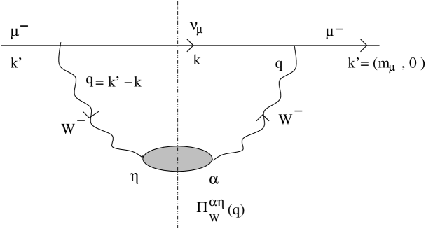
Figure 6: Diagrammatic representation of the muon (at rest) selfenergy in nuclear matter.

The spin averaged muon decay width, in an infinite nuclear matter of densities $\rho_{p}(r)$ and $\rho_{n}(r)$, is related to the imaginary part of the selfenergy (see Fig. 6), $\Sigma_{\mu}^{r}\left(\rho_{p}(r),\rho_{n}(r)\right)$, of a muon at rest and spin $r$ in the medium by

$$\hat{\Gamma}\left(\rho_{p}(r),\rho_{n}(r)\right)=-\frac{1}{m_{\mu}}{\rm Im}\Sigma_{\mu}\left(\rho_{p}(r),\rho_{n}(r)\right),\qquad\Sigma_{\mu}=\frac{1}{2}\sum_{r}\Sigma_{\mu}^{r}$$ (59)

To evaluate the imaginary part of the selfenergy associated to the diagram of Fig. 6, the intermediate states are placed on shell in the integration over the internal variables. These states are those crossed by the dash–dotted line in Fig. 6. The evaluation of the $\mu-$selfenergy is almost identical to that of a neutrino in Fig. 1, and thus we obtain from Eq. (14),

$$\hat{\Gamma}\left(\rho_{p}(r),\rho_{n}(r)\right)=-\frac{1}{m_{\mu}}\frac{4G}{\sqrt{2}M^{2}_{W}}\int\frac{d^{3}k}{(2\pi)^{3}}\frac{\Theta(q^{0})}{2|\vec{k}\,|}~{}{\rm Im}\left\{\overline{\Pi}^{\mu\eta}_{W}\left(q;\rho_{p}(r),\rho_{n}(r)\right)L_{\mu\eta}\right\}$$ (60)

with $q^{0}=m_{\mu}-|\vec{k}\,|$ and $|\vec{q}\,|=|\vec{k}\,|$. For kinematical reasons, only the QE part of the $W^{-}-$selfenergy will contribute to the muon decay width and thus we find

$$\hat{\Gamma}\left(\rho_{p}(r),\rho_{n}(r)\right) = \frac{G^{2}\cos^{2}\theta_{C}}{m_{\mu}}\int\frac{d^{3}k}{(2\pi)^{3}}\frac{1}{2|\vec{k}\,|}L_{\mu\eta}{\cal T}^{\mu\eta}\left(q;\rho_{p},\rho_{n}\right)$$ (61)

$$= \frac{G^{2}\cos^{2}\theta_{C}}{2\pi^{2}}\int_{0}^{+\infty}\vec{k}^{\,2}\left(-t_{1}+\frac{t_{2}}{2}+|\vec{k}\,|t_{3}+\frac{m_{\mu}^{2}}{2}t_{4}+m_{\mu}t_{5}\right)d|\vec{k}\,|$$

where the tensor ${\cal T}^{\mu\nu}$ is defined as

$${\cal T}^{\mu\nu}\left(q;\rho_{p},\rho_{n}\right) = -\frac{1}{4M^{2}}\Big{\{}2\Theta(q^{0})\int\frac{d^{3}p}{(2\pi)^{3}}\frac{M}{E(\vec{p})}\frac{M}{E(\vec{p}+\vec{q})}\Theta(k_{F}^{p}(r)-|\vec{p}~{}|)\Theta(|\vec{p}+\vec{q}~{}|-k_{F}^{n}(r))$$ (62)

$$\times (-\pi)\delta(q^{0}+E(\vec{p})-E(\vec{p}+\vec{q}~{}))A^{\mu\nu}_{\rm RPA}(p,q)|_{p^{0}=E(\vec{p})~{}}\Big{\}}$$

$$\equiv t_{1}g^{\mu\nu}+t_{2}l^{\mu}l^{\nu}+{\rm i}t_{3}\epsilon^{\mu\nu\alpha\beta}l_{\alpha}q_{\beta}+t_{4}q^{\mu}q^{\nu}+t_{5}\left(l^{\mu}q^{\nu}+l^{\nu}q^{\mu}\right),\qquad{\rm with}~{}l^{\mu}=(1,\vec{0}).$$

The similitude of the above equation with Eq. (28) is clear. As in this latter case, the $d^{3}p$ integrations in Eq. (62) can be done analytically (see Sect. B of the Appendix) and all of them are determined by the imaginary part of the relativistic isospin asymmetric Lindhard function, $\overline{U}_{R}(q,k_{F}^{n},k_{F}^{p})$. For a non-relativistic Fermi gas, the decay width is easily obtained from Eq. (62) by replacing the factors $M/E(\vec{p})$ and $M/E(\vec{p}+\vec{q})$ by one. Analytical expressions can be now found in the Sect. C of the Appendix. FSI effects can be also taken into account by performing the substitution of Eq. (53).

Thus, both the muon decay process in the medium and the electroweak inclusive nuclear reactions $\nu_{l}(k)+\,A_{Z}\to l^{-}(k^{\prime})+X$ in the QE regime are sensitive to the same physical features, $W^{\pm}pn-$vertex, and RPA and FSI effects. However, in the muon-atom decay only very small nuclear excitation energies are explored, 0–25 MeV, while in the latter processes higher nuclear excitation energies can be tested by varying the incoming neutrino momentum.

The $1s$ muon binding energy, $B_{\mu}^{1s}>0$, can be taken into account, by replacing $m_{\mu}\to\hat{m}_{\mu}=m_{\mu}-B_{\mu}^{1s}$. This replacement leads to extremely small (significant) changes for light (heavy) nuclei, where $B^{1s}_{\mu}$ is of the order of 0.1 MeV (10 MeV), see Table 1.

Finally, the correct energy balance in the decay can be enforced in the LFG by replacing

$$q^{0}\to q^{0}-\left(\overline{Q}-\overline{Q}^{\rm LFG}(r)\right)=\hat{m}_{\mu}-|\vec{k}\,|-\left(\overline{Q}-\overline{Q}^{\rm LFG}(r)\right)$$ (63)

in Eqs. (61) and (62).

VI Results

Firstly, we compile in Table 1 the input used for the different nuclei studied in this work. Nuclear masses and charge densities are taken from Refs. Fi96 and Ja74 , respectively. For each nucleus, we take the neutron matter density approximately equal (but normalized to $N$) to the charge density, though we consider small changes, inspired by Hartree-Fock calculations with the density-matrix expansion Ne75 and corroborated by pionic atom data GNO92 . However charge (neutron) matter densities do not correspond to proton (neutron) point–like densities because of the finite size of the nucleon. This is taken into account by following the procedure outlined in Section 2 of Ref. GNO92 (see Eqs. (12)-(14) of this reference).

Nucleus	$R_{p}$ [fm]	$R_{n}$[fm]	$a$ [fm]∗	$Q$ [MeV]	$\overline{Q}$ [MeV]	$B_{\mu}^{1s}$ [MeV]
12C	1.692	1.692	1.082	16.827	13.880	0.100
16O	1.833	1.833	1.544	14.906	10.931	0.178
18O	1.881	1.975	1.544	1.144	14.413	0.178
23Na	2.773	2.81	0.54	3.546	4.887	0.336
40Ca	3.51	3.43	0.563	13.809	1.822	1.064
44Ca	3.573	3.714	0.563	3.142	6.170	1.063
75As	4.492	4.64	0.58	0.353	1.688	2.624
112Cd	5.38	5.58	0.58	2.075	4.462	4.861
208Pb	6.624	6.890	0.549	2.368	5.512	10.510

(*) The parameter $a$ is dimensionless for the MHO density form.

Table 1: Charge ($R_{p},a$), neutron matter ($R_{n},a$) density parameters, $Q,\overline{Q}-$values and negative muon binding energies for different nuclei. For carbon and oxygen we use a modified harmonic oscillator (MHO) density, $\rho(r)=\rho_{0}(1+a(r/R)^{2})\exp(-(r/R)^{2})$, while for the rest of the nuclei, a two-parameter Fermi distribution, $\rho(r)=\rho_{0}/(1+\exp((r-R)/a))$, was used.

VI.1 Inclusive Neutrino Reactions at Low Energies

In this subsection we present results obtained by using non-relativistic kinematics for the nucleons. We do not include FSI effects, since in Sect. III.3 we made the approximation of setting to zero Im$\Sigma$ for the hole states. For low nuclear excitation energies ($\leq 60$), this approximation is not justified, because the imaginary part of the selfenergy of particle and hole states are comparable FO92 . The inclusion of FSI effects would lead to a quenching of the QE peak of the bare ph calculation, and a spreading of the strength GNO97 ; Bl01 ; Ma03 ; Am04 ; RPC . However FSI effects on integrated quantities are small. From the results of the next subsection we estimate in $\sim 5$–10% the theoretical error of the integrated cross sections and total muon capture rates presented in this subsection.

The processes studied in this subsection explore quite low nuclear excitation energies ($\leq$ 25–30 MeV), and hence one might expect that a proper finite nuclei treatment could be in order. Indeed, these processes are sensitive to the excitation of giant resonances Au02 ; Au97 ; Vol00 ; Ko03 . As mentioned in the Introduction, our purpose is to describe the interaction of neutrinos and antineutrinos with nuclei at higher energies (nuclear excitation energies of the order of 100–600 MeV) of interest for future neutrino oscillation experiments. However, our model provides a good description of the low energy inclusive measurements analyzed in this subsection. RPA correlations play an essential role and lead to reductions as large as a factor of two. We should remind that the effective interaction appearing in the RPA series was fitted in Ref. Sp77 to giant resonances, and thus our approach incorporates the mechanism which produces those resonances in finite nuclei.

At low energies, finite nuclei effects are expected to be sizeable for outgoing lepton energy distributions. There exist discrete and resonance state peaks, and the continuum distribution significantly differs from the LFG one. However, the integrated strength over energies, including the discrete state and resonance contributions, remains practically unchanged, which explains the success of our model to describe integrated-inclusive magnitudes. A clear example of this can be found in Ref. Am04 where the inclusive decay width of muonic atoms by using a shell model with final neutron states lying both in the continuum and in the discrete spectrum are calculated. The results are compared with those obtained from a LFG model. Both models are in quite good agreement within a few percent when the shell model density is used in the LFG calculation. Being an integrated, inclusive observable, the total capture width is quite independent of the fine details of the nuclear wave functions. Similar conclusions were reached in the study of the radiative pion capture in nuclei, $\left(A_{Z}-\pi^{-}\right)_{\rm bound}\to\gamma+X$, performed in Ref. RPC . There, the predictions of a continuum shell model were also extensively compared to those deduced from a LFG picture of the nucleus. The differences found, among the integrated decay widths predicted by both approaches, were, at most, of the order of 4% (see Table 5 of first entry in Ref. RPC ).

Figure 7: Predictions for the LSND measurement of the ¹²C $(\nu_{\mu},\mu^{-})X$ reaction (left panels) and the ¹²C $(\nu_{e},e^{-})X$ reaction near threshold (right panels). Results have been obtained by using non-relativistic kinematics for the nucleons and without FSI. Top: $\nu_{\mu}$ and $\nu_{e}$ cross sections multiplied by the neutrino fluxes, as a function of the neutrino energy. In addition to the RPA calculation (solid line), we show results without RPA correlations and Coulomb corrections (dotted line), and also (dashed line) the low density limit of Eq. (31). Middle: Differential muon and electron neutrino cross sections at $E_{\nu_{\mu}}=179.5$ MeV (left) and $E_{\nu_{e}}=46.2$ MeV (right), as a function of the energy transfer. Bottom: Neutrino spectra from Al95 (left) and Eq. (65) (right).

	LDT	Pauli+$Q$	RPA	SM HT00	SM Vol00	CRPA Ko03	Exp
							LSND’95 Al95	LSND’97 At97	LSND’02 Auexp02
$\overline{\sigma}$ $(\nu_{\mu},\mu^{-})$	66.1	20.7	11.9	13.2	15.2	19.2	$8.3\pm 0.7\pm 1.6$	$11.2\pm 0.3\pm 1.8$	$10.6\pm 0.3\pm 1.8$
							KARMEN KARMEN	LSND LSND	LAMPF LAMPF
$\overline{\sigma}$ $(\nu_{e},e^{-})$	5.97	0.19	0.14	0.12	0.16	0.15	$0.15\pm 0.01\pm 0.01$	$0.15\pm 0.01\pm 0.01$	$0.141\pm 0.023$

Table 2: Experimental and theoretical flux averaged ${}^{12}{\rm C}(\nu_{\mu},\mu^{-})X$ and ${}^{12}{\rm C}(\nu_{e},e^{-})X$ cross sections in 10^-40 cm² units. We label our predictions as in Fig. 7. We also quote results from other calculations (see text for details).

VI.1.1 The Inclusive Reactions ${}^{12}{\rm C}(\nu_{\mu},\mu^{-})X$ and ${}^{12}{\rm C}(\nu_{e},e^{-})X$ Near Threshold

In order to compare with the experimental measurements we calculate flux averaged cross sections

$$\overline{\sigma}=\frac{1}{{\cal N}}\int_{E_{\nu}^{\rm min}}^{E_{\nu}^{\rm max}}dE_{\nu}\sigma(E_{\nu})W(E_{\nu}),\quad{\cal N}=\int_{E_{\nu}^{\rm min}}^{E_{\nu}^{\rm max}}W(E_{\nu})dE_{\nu},$$ (64)

In the LSND experiment at Los Alamos, the inclusive ${}^{12}{\rm}C(\nu_{\mu},\mu^{-})X$ cross section was measured using a pion decay in flight $\nu_{\mu}$ beam, with energies ranging from zero to 300 MeV, and a large liquid scillantor detector Al95 ; At97 ; Auexp02 . The muon neutrino spectrum, $W(E_{\nu})$, is taken from Ref. Al95 and it is plotted in the left bottom panel of Fig. 7. We fix $E_{\nu}^{\rm min}$ and $E_{\nu}^{\rm max}$ to 123.1 and 300 MeV, respectively. The electron neutrino beams used in experiments (LAMPF, KARMEN, etc.) have relatively low energies. Such neutrinos do not constitute a monochromatic beam, and their spectrum is plotted in the right bottom panel of Fig. 7. The bare ph strength spreading due to the FSI might affect the inclusive, flux averaged cross-section because of the energy variations in the neutrino flux. As an illustration, if some of the strength is shifted to higher energies then some of the low-energy neutrinos will not be able to excite it, compared with the case when the strength is not spread out. Of course these effects are not very large, because some strength is also moved to lower energies and compensates this. These uncertainties contribute to the $\sim 5$–10% theoretical error mentioned above.

Our results for the ${}^{12}{\rm C}(\nu_{\mu},\mu^{-})X$ and ${}^{12}{\rm C}(\nu_{e},e^{-})X$ reactions near threshold are presented in Fig. 7 and Table 2. As can be seen in the table, the agreement to data is remarkable. Nuclear effects turn out to be essential, and thus the simple prescription of multiplying by a factor of six (the number of neutrons of ¹²C) the free space $\nu_{l}n\to pl^{-}$ cross section overestimates the flux averaged cross sections by a factor of 5 and of 40 for the muon and electron neutrino induced reactions, respectively. The inclusion of Pauli blocking and the use of the correct energy balance in the reaction lead to much better results, but the cross sections are still badly overestimated. Only once RPA and Coulomb corrections are included a good description of data is achieved. RPA correlations reduce the flux averaged cross sections by about a factor of two, while Coulomb distortion significantly enhances them, in particular for the electron neutrino reaction where this enhancement is of about 30%.

In Table 2, a few selected theoretical calculations (large basis shell model (SM) results of Refs. Vol00 ; HT00 and the continuum RPA (CRPA) ones from Ref. Ko03 ) are also quoted. Our approach might look simplified with respect to the ones just mentioned, but in fact it is also an RPA approach built up from single particle states of an uncorrelated Fermi sea. This method in practice is a very accurate tool when the excitation energy is sufficiently large such that relatively many states contribute to the process. Obviously, because of its nature, the method only applies to inclusive processes and it is not meant to evaluate transitions to discrete states. The adaptation of the method to finite nuclei via the LDA has proved to be a rather precise technique to deal with inclusive photonuclear reactions CO92 and response functions in electron scattering GNO97 . The effective ph($\Delta$h)-ph($\Delta$h) interaction used in the RPA series has been successfully employed in different processes GNO97 ; CO92 ; pion . There are two distinctive features of this interaction in the $S=T=1$ channel, which are not incorporated in most of the finite nuclei approaches: i) it incorporates explicit pion and rho exchanges and thus the force in this channel is splited into longitudinal and transverse parts, and ii) it includes resonance $\Delta$ degrees of freedom. The inclusion of $\Delta$h components in the RPA series reduces the LSND flux averaged ¹²C $(\nu_{\mu},\mu^{-})X$ cross section by about a 15%, while the reduction factor is about four times smaller for the electron neutrino reaction, because in this latter case, the larger contributions to the flux averaged ¹²C$(\nu_{e},e^{-})X$ cross section comes from very low ($\leq 20$ MeV) nuclear excitation energies (see Fig. 7). In addition, a correct tensorial treatment of the RPA hadronic tensor is also important, and it explains the bulk of the existing differences between our results and those obtained in Ref. Si92 (see Subsect. III.1 for details). As a matter of example, in Ref. Si92 a value of $16.7\pm 1.4\times 10^{-40}~{}{\rm cm}^{2}$ is predicted for the LSND flux averaged ¹²C$(\nu_{\mu},\mu^{-})X$ cross section. This value is about a 40% higher than our result, despite of using quite similar ph($\Delta$h)-ph($\Delta$h) effective interactions. Differences are significantly smaller for the electron neutrino flux averaged cross section, since this reaction is sensitive to quite lower energies.

In the middle panels of Fig. 7, we plot the outgoing lepton energy distribution for an incoming neutrino energy near the maximum of $\sigma(E_{\nu})W(E_{\nu})$ (top panels). We see in these plots the range of energies transferred ($E_{\nu}-E^{\prime}_{l}-Q$) to the daughter nucleus: 25-30 MeV for the muon neutrino reaction and less than 10 MeV for the electron neutrino process. Finite nuclei distributions will present some discrete state and narrow resonance peaks, but the integrated strength over energies would not be much affected though, as we have already discussed.

VI.1.2 Total Nuclear Capture Rates for Negative Muons

	Pauli+$\overline{Q}$ $[10^{4}\,s^{-1}]$	RPA $[10^{4}\,s^{-1}]$	Exp $[10^{4}\,s^{-1}]$	$\left(\Gamma^{\rm Exp}-\Gamma^{\rm Th}\right)/\Gamma^{\rm Exp}$
12C	5.42	3.21	$3.78\pm 0.03$	$-$0.15
16O	17.56	10.41	$10.24\pm 0.06$	$-0.02$
18O	11.94	7.77	$8.80\pm 0.15$	$-$0.12
23Na	58.38	35.03	$37.73\pm 0.14$	$-$0.07
40Ca	465.5	257.9	$252.5\pm 0.6$	$-0.02$
44Ca	318	189	$179\pm 4$	$-0.06$
75As	1148	679	609$\pm 4$	$-0.11$
112Cd	1825	1078	1061$\pm 9$	$-0.02$
208Pb	1939	1310	1311$\pm 8$	$-$$0.00$

Table 3: Experimental and theoretical total muon capture widths for different nuclei. Data are taken from Ref. Su87 , and when more than one measurement is quoted in Su87 , we use a weighted average: $\overline{\Gamma}/\sigma^{2}=\sum_{i}\Gamma_{i}/\sigma_{i}^{2}$, with $1/\sigma^{2}=\sum_{i}1/\sigma_{i}^{2}$. Theoretical results have been obtained by using non-relativistic kinematics for the nucleons (Sect. C of the Appendix). To illustrate the role played by the RPA correlations, we quote two different theoretical results: i) Pauli+$\overline{Q}$ obtained from Eq. (62) without including FSI effects and RPA correlations (i.e., replacing $A^{\mu\nu}_{\rm RPA}$ by $A^{\mu\nu}$ in Eq. (62)), but taking into account the value of $\overline{Q}$; ii) the full calculation, including all nuclear effects with the exception of FSI, presented in Sect.V, and denoted as RPA. Finally, in the last column we show the relative discrepancies existing between the theoretical predictions given in the third column and data.

Figure 8: Inclusive muon capture differential width from ¹²C, as a function of the outgoing neutrino energy (top axis) and of the energy transfer (bottom axis). Non-relativistic kinematics has been used for the nucleons. The two calculations are labeled as in Table 3.

After the success in describing the LSND measurement of the reaction ¹²C $(\nu_{\mu},\mu^{-})X$ near threshold, it seems natural to further test our model by studying the closely related process of inclusive muon capture in ¹²C. Furthermore, and since there are abundant and accurate measurements of nuclear inclusive muon capture rates through the whole periodic table, we have also calculated muon capture widths for a few selected nuclei, which will be also studied below in Sect. VI.2. Our results are compiled in Table 3. Data are quite accurate, with precisions smaller than 1%, quite far from the theoretical uncertainties of any existing model. Medium polarization effects (RPA correlations), once more, are essential to describe the data, as was already shown in Ref. Ch90 . Despite the huge range of variation of the capture widths, the agreement to data is quite good for all studied nuclei, with discrepancies of about 15% at most. It is precisely for ¹²C, where we find the greatest discrepancy with experiment. Nevertheless, our model provides one of the best existing combined description of the inclusive muon capture in ¹²C and the LSND measurement of the reaction ¹²C $(\nu_{\mu},\mu^{-})X$ near threshold Ko03 .

Finally, in Fig. 8 we show the outgoing $\nu_{\mu}$ energy distribution from muon capture in ¹²C, which ranges from 70 to 90 MeV. The energy transferred to the daughter nucleus (¹²B) ranges from 0 to 20 MeV. We also show in the figure the medium polarization effect on the differential decay rate. As already mentioned, the shape of the curves in Fig. 8 will significantly change if a proper finite nuclei treatment is carried out, with the appearance of narrow peaks, but providing similar values for the integrated widths Am04 .

VI.2 Inclusive QE Neutrino and Antineutrino Reactions at Intermediate Energies

Figure 9: RPA and Coulomb (CB) corrections to electron and muon neutrino and antineutrino QE cross sections for different nuclei, as a function of the neutrino energy. A relativistic treatment of the nucleons is undertaken and FSI effects are not considered. $R_{\rm RPA+CB}$ is defined as $(\sigma_{\rm RPA+CB}-\sigma_{0})/\sigma_{0}$, where $\sigma_{0}$ does not include RPA and Coulomb corrections, while $\sigma_{\rm RPA+CB}$ includes these nuclear effects.

Figure 10: Electron and muon neutrino and antineutrino inclusive QE cross sections and ratios for different nuclei, at intermediate energies. Results have been obtained with the full model without FSI, and using relativistic kinematics for the nucleons. For comparison we also show results obtained in the free space (low density limit, LDT, Eq. (31)).

In this subsection we will present results on muon and electron neutrino and antineutrino induced reactions in several nuclei for intermediate energies, where the predictions of the model developed in this work are reliable, not only for integrated cross sections, as in the previous subsection, but also for differential cross sections. We will present results for incoming neutrino energies within the interval 150-400 (250-500) MeV for electron (muon) species. The use of relativistic kinematics for the nucleons leads to moderate reductions of both neutrino and antineutrino cross sections, ranging these reductions in the interval 4-9%, at the intermediate energies considered in this work. Such corrections do not depend significantly on the considered nucleus.

In Fig 9, the effects of RPA and Coulomb corrections are studied as a function of the incoming neutrino/antineutrino energy. These corrections are important (20-60%), both for neutrino and antineutrino reactions, in the whole range of considered energies. RPA correlations reduce the cross sections, and we see large effects, specially at lower energies. The RPA reductions become smaller as the energy increases. Nevertheless for the higher energies considered (500 and 400 MeV for muon and electron neutrino reactions, respectively) we still find suppressions of about 20-30%. Coulomb distortion of the outgoing charged lepton enhances (reduces) the cross sections for neutrino (antineutrino) processes. Coulomb effects decrease with energy. For antineutrino reactions, the combined effect of RPA and Coulomb corrections have a moderated dependence on $A$ and $Z$. Coulomb corrections reduce the outgoing positive charged lepton effective momentum inside of the nuclear medium. Thus, the phase space correction factor $|\vec{{\cal K}}^{\,\prime}(r)|\hat{E}^{\prime}_{l}(r)/|\vec{k}^{\,\prime}|E^{\prime}_{l}$ is smaller than one and the cross section gets smaller. This effect, obviously grows with $Z$. On the other hand, the RPA suppression decreases when the lepton effective momentum increases and it grows with $A$. The combined effect explains the nuclear dependence found in the antineutrino plots. At the higher energy end the $A-$dependence becomes milder, since Coulomb distortion becomes less important. In the case of neutrinos, the increase of the cross section due to Coulomb cancels out partially with the RPA reduction. Finally, the existing differences between electron and muon neutrino/antineutrino plots are due to the different momenta of an electron and a muon with the same energy.

In Fig. 10, we show electron and muon neutrino and antineutrino inclusive QE cross sections and ratios for different nuclei, as a function of the incoming lepton energy. Results have been obtained with the full model presented in Sect.III, including all nuclear effects with the exception of FSI, and using relativistic kinematics for the nucleons. Neutrino cross sections scale with $N$ (number of neutrons) reasonably well, while there exist important departures from a $Z$ (number of protons) scaling rule for antineutrino cross sections. These departures can be easily understood from the discussion of Fig.9. To better disentangle medium effects, the free space neutrino/antineutrino nucleon cross section multiplied by the number of neutrons or protons is also depicted in the plots.

Figure 11: Muon neutrino and antineutrino relativistic QE differential cross sections from different nuclei and several $\nu_{\mu},{\bar{\nu}}_{\mu}$ energies. Results, denoted as ’Pauli+$Q$’ or ’Pauli+$\overline{Q}$’ have been obtained in ¹²C and do not include RPA, FSI and Coulomb effects, while the rest of results have been obtained with the full model without FSI.

In Fig. 11 we show muon neutrino and antineutrino inclusive QE differential cross sections as a function of the energy transfer, for different isoscalar nuclei and different incoming lepton energies. We see an approximate $A-$scaling and once more the important role played by the medium polarization effects. Similar results (not shown in the figure) are obtained from electron species.

The double differential cross section $d\sigma/dE^{\prime}_{l}d|\vec{q}\,|$ for the muon neutrino reaction in calcium is shown in Fig. 12. In the top panel, we compare the lepton scattering angle distribution for three different values of the energy transfer. As usual in QE processes, the peaks of the distributions are placed in the vicinity of $|\vec{q}\,|=\sqrt{2Mq^{0}}$. In the bottom panel, we show FSI effects on the differential cross section for one of the energies ($E_{l}^{\prime}=228.6$ MeV) studied in the upper panel. We also show the effects of using relativistic kinematics for the nucleons. As anticipated, FSI provides a broadening and a significant reduction of the strength of the QE peak. Nevertheless the $|\vec{q}~{}|$ integrated cross section is only slightly modified (a reduction of about 2.5% when RPA corrections are not considered and only about 1% enhancement when they are included).

Figure 12: Muon neutrino differential cross sections in calcium as a function of the lepton scattering angle (top) and of the momentum transfer (bottom). The neutrino energy is 371.8 MeV. Top: Cross sections, without FSI and using relativistic kinematics for the nucleons, at different muon energies. Crosses have been obtained without RPA and Coulomb effects, while the curves have been obtained with the full model (up to FSI effects). Bottom: Cross sections, for a muon energy of 228.6 MeV, obtained by using relativistic (long dashed line,’REL’) and non-relativistic nucleon kinematics. In this latter case, we present results with (solid line , ’FSI’) and without (short dashed line, ’NOREL’) FSI effects. For the three cases, we also show the effect of taking into account RPA and Coulomb corrections (lower lines at the peak). The areas (in units of 10^-40 cm²/MeV) below the curves are 3.50 (REL), 3.87 (NOREL) and 3.77 (FSI) when RPA and Coulomb corrections are not considered, and 3.13 (REL), 3.49 (NOREL) and 3.53 (FSI) when these nuclear effects are taken into account.

In Fig. 13 we plot double differential cross sections for fixed momentum transfer, as a function of the excitation energy. We show neutrino and antineutrino cross sections from ¹⁶O. FSI effects are not considered in the top panel, and one finds the usual QE shape, with peaks placed, up to relativistic corrections, in the neighborhood of $\vec{q}^{\,2}/2M$. Once more, medium polarization effects are clearly visible. FSI corrections are studied in the bottom panel, and we find the expected broadening of the QE peak, but the integrated cross sections remain almost unaltered.

Figure 13: $\nu_{e}$ and $\overline{\nu}_{e}$ differential cross sections in ¹⁶O as a function of the excitation energy, for fixed values of the momentum transfer and $E_{\nu,\overline{\nu}}=400$ MeV. Top: Results obtained from the full relativistic model without FSI, with (’RPA’) and without RPA and Coulomb corrections (’Pauli+$Q(\overline{Q})$’). Bottom: Results obtained by using relativistic (long dashed line, ’REL’) and non-relativistic nucleon kinematics. In this latter case, we present results with (solid line, ’FSI’) and without (short dashed line, ’NOREL’) FSI effects. For the three cases, we also show the effect of taking into account RPA and Coulomb corrections (lower lines at the peak). The areas (in units of 10^-40 cm²/MeV) below the curves are 1.02 (REL), 1.13 (NOREL) and 1.01 (FSI) when RPA and Coulomb corrections are not considered, and 0.79 (REL), 0.90 (NOREL) and 0.85 (FSI) when these nuclear effects are taken into account.

Finally, in Table 4 we compile muon and electron neutrino and antineutrino inclusive QE integrated cross sections from oxygen. We present results for relativistic and non-relativistic nucleon kinematics and in this latter case, we present results with and without FSI effects. Though FSI change importantly the shape of the differential cross sections, it plays a minor role when one considers total cross sections. When medium polarization effects are not considered, FSI provides significant reductions (13-29%) of the cross sections Bl01 . However, when RPA corrections are included the reductions becomes more moderate, always smaller than 7%, and even there exist some cases where FSI enhances the cross sections. This can be easily understood by looking at Fig. 14, where we show the differential cross section as a function of the energy transfer for $E_{\nu}=375$ MeV. There, we see that FSI increases the cross section for high energy transfer. But for nuclear excitation energies higher than those around the QE peak, the RPA corrections are certainly less important than in the peak region. Hence, the RPA suppression of the FSI distribution is significantly smaller than the RPA reduction of the distribution determined by the ordinary Lindhard function.

$E_{\nu}$ [MeV]		$\sigma\left({}^{16}{\rm O}(\nu_{\mu},\mu^{-}X)\right)~{}[10^{-40}$ cm2]			$\sigma\left({}^{16}{\rm O}({\bar{\nu}}_{\mu},\mu^{+}X)\right)~{}[10^{-40}$ cm2]
		REL	NOREL	FSI	REL	NOREL	FSI
500	Pauli + $Q(\overline{Q})$	460.0	497.0	431.6	155.8	168.4	149.9
	RPA	375.5	413.0	389.8	113.4	126.8	129.7
375	Pauli + $Q(\overline{Q})$	334.6	354.8	292.2	115.1	122.6	105.0
	RPA	243.1	263.9	243.9	79.8	87.9	87.5
250	Pauli + $Q(\overline{Q})$	155.7	162.2	122.5	63.4	66.4	52.8
	RPA	94.9	101.9	93.6	38.8	42.1	40.3
$E_{\nu}$ [MeV]		$\sigma\left({}^{16}{\rm O}(\nu_{e},e^{-}X)\right)~{}[10^{-40}$ cm2]			$\sigma\left({}^{16}{\rm O}({\bar{\nu}}_{e},e^{+}X)\right)~{}[10^{-40}$ cm2]
		REL	NOREL	FSI	REL	NOREL	FSI
310	Pauli + $Q(\overline{Q})$	281.4	297.4	240.6	98.1	104.0	87.2
	RPA	192.2	209.0	195.2	65.9	72.4	73.0
220	Pauli + $Q(\overline{Q})$	149.5	156.2	121.2	60.7	63.6	51.0
	RPA	90.1	97.3	92.8	36.8	40.0	40.2
130	Pauli + $Q(\overline{Q})$	37.0	38.3	28.8	21.1	21.9	16.9
	RPA	20.6	22.3	23.3	10.9	11.9	12.8

Table 4: Muon (top) and electron (bottom) neutrino (left) and antineutrino (right) inclusive QE integrated cross sections from oxygen. We present results for relativistic (’REL’) and non-relativistic nucleon kinematics. In this latter case, we present results with (’FSI’) and without (’NOREL’) FSI effects. Results, denoted as ’RPA’ and ’Pauli+$Q(\overline{Q})$’ have been obtained with and without including RPA correlations and Coulomb corrections, respectively.

Figure 14: Muon neutrino QE differential cross sections in oxygen as a function of the energy transfer. The neutrino energy is 375 MeV. We show results for relativistic (long dashed line, ’REL’) and non-relativistic nucleon kinematics. In this latter case, we present results with (solid line, ’FSI’) and without (short dashed line, ’NOREL’) FSI effects. We also show the effect of RPA and Coulomb corrections (lower lines at the peak). The integrated cross sections can be found in Table 4.

VII Conclusions

The model presented in this paper, which is a natural extension of previous works GNO97 ; CO92 ; OTW82 ; pion on electron, photon and pion dynamics in nuclei, should be able to describe inclusive QE neutrino and antineutrino nuclear reactions at intermediate energies of interest for future neutrino oscillation experiments. Even though the scarce existing data involve very low nuclear excitation energies, for which specific details of the nuclear structure might play a role, our model provides one of the best existing combined description of the inclusive muon capture in ¹²C and of the measurements of the ¹²C $(\nu_{\mu},\mu^{-})X$ and ¹²C $(\nu_{e},e^{-})X$ reactions near threshold. Inclusive muon capture from other nuclei is also successfully described by the model.

The inclusion of RPA effects, in particular the nuclear renormalization of the axial current, turned out to be extremely important to obtain an acceptable description of data. This had been already pointed out in Refs. Ch90 ; Au02 ; Si92 ; Ko03 , and it is a distinctive feature of nuclear reactions at intermediate energies GNO97 ; CO92 ; OTW82 ; pion . On the other hand FSI effects, though produce significantly changes in the shape of differential cross sections, lead to minor changes for integrated cross sections, comparable to the theoretical uncertainties, once RPA corrections are also taken into account.

The natural extension of this work is the study of higher transferred energies to the nucleus, also relevant for the analysis of future experiments aiming at determining the neutrino oscillation parameters with high precision. For those energies, the production of real pions and the excitation of the $\Delta(1232)$ or higher resonances will be contributions to the inclusive neutrino–nucleus cross section comparable to the QE one, or even larger.

Appendix A CC Nucleon Tensor

A.1 Impulse Approximation

Performing the traces in Eq. (27) and taking into account that in Eq. (28) both the particle and the hole nucleons are on the mass shell ($p^{2}=(p+q)^{2}=M^{2},~{}2p\cdot q+q^{2}=0$), one finds

$$A^{\mu\nu}(p,q) = 16(F_{1}^{V})^{2}\left\{(p+q)^{\mu}p^{\nu}+(p+q)^{\nu}p^{\mu}+\frac{q^{2}}{2}g^{\mu\nu}\right\}+2q^{2}(\mu_{V}F_{2}^{V})^{2}\left\{4g^{\mu\nu}-4\frac{p^{\mu}p^{\nu}}{M^{2}}-2\frac{p^{\mu}q^{\nu}+q^{\mu}p^{\nu}}{M^{2}}\right.$$ (66)

$$- \left.q^{\mu}q^{\nu}(\frac{4}{q^{2}}+\frac{1}{M^{2}})\right\}-16F_{1}^{V}\mu_{V}F_{2}^{V}(q^{\mu}q^{\nu}-q^{2}g^{\mu\nu})+4G_{A}^{2}\left\{2p^{\mu}p^{\nu}+q^{\mu}p^{\nu}+p^{\mu}q^{\nu}+g^{\mu\nu}(\frac{q^{2}}{2}-2M^{2})\right.$$

$$- \left.\frac{2M^{2}(2m_{\pi}^{2}-q^{2})}{(m_{\pi}^{2}-q^{2})^{2}}q^{\mu}q^{\nu}\right\}-16{\rm i}G_{A}\left(\mu_{V}F_{2}^{V}+F_{1}^{V}\right)\epsilon^{\mu\nu\alpha\beta}q_{\alpha}p_{\beta}$$

The above tensor admits a decomposition of the type

$$A^{\mu\nu}(p,q)=a_{1}g^{\mu\nu}+a_{2}\left(p^{\mu}p^{\nu}+\frac{p^{\mu}q^{\nu}+p^{\nu}q^{\mu}}{2}\right)+{\rm i}a_{3}\epsilon^{\mu\nu\alpha\beta}p_{\alpha}q_{\beta}+a_{4}q^{\mu}q^{\nu}$$ (67)

and from Eq. (66) we have

$$a_{1}(q^{2}) = 8q^{2}\left\{(F_{1}^{V}+\mu_{V}F_{2}^{V})^{2}+G_{A}^{2}\left(\frac{1}{4}-\frac{M^{2}}{q^{2}}\right)\right\}$$

$$a_{2}(q^{2}) = 32(F_{1}^{V})^{2}-8(\mu_{V}F_{2}^{V})^{2}\frac{q^{2}}{M^{2}}+8G_{A}^{2}$$

$$a_{3}(q^{2}) = 16G_{A}(F_{1}^{V}+\mu_{V}F_{2}^{V})$$

$$a_{4}(q^{2}) = -\frac{8q^{2}}{M^{2}}(\mu_{V}F_{2}^{V})^{2}\left(\frac{M^{2}}{q^{2}}+\frac{1}{4}\right)-\frac{8M^{2}G_{A}^{2}}{m_{\pi}^{2}-q^{2}}\left(\frac{q^{2}}{m_{\pi}^{2}-q^{2}}+2\right)-16F_{1}^{V}\mu_{V}F_{2}^{V}$$ (68)

A.2 RPA Corrections

Taking $\vec{q}$ in the $z$ direction and after performing the RPA sum of Fig. 3, we find, neglecting corrections of order ${\cal O}\left(k_{F}\vec{p}^{\,2}/M^{2},k_{F}\vec{p}^{\,\prime 2}/M^{2},k_{F}q^{0}/M\right)$

$$\frac{A^{00}_{\rm RPA}}{4M^{2}} = 8(F_{1}^{V})^{2}\left\{\underline{\bf C_{N}}\,\left(\frac{E(\vec{p}\,)}{M}\right)^{2}+\frac{q^{2}/4+q^{0}E(\vec{p}\,)}{M^{2}}\right\}-2\frac{q^{2}}{M^{2}}(\mu_{V}F_{2}^{V})^{2}\left\{\frac{\vec{p}^{\,2}+q^{0}E(\vec{p})+(q^{0})^{2}/4}{M^{2}}+\frac{(q^{0})^{2}}{q^{2}}\right\}$$ (69)

$$- 4\underline{\bf C_{N}}F_{1}^{V}\mu_{V}F_{2}^{V}\frac{\vec{q}^{\,2}}{M^{2}}+2G_{A}^{2}\left\{\frac{q^{0}E(\vec{p})+q^{2}/4+\vec{p}^{\,2}}{M^{2}}-\underline{\bf C_{L}}\,\frac{(q^{0})^{2}}{m_{\pi}^{2}-q^{2}}\left(\frac{q^{2}}{m_{\pi}^{2}-q^{2}}+2\right)\right\}$$

$$\frac{A^{0z}_{\rm RPA}}{4M^{2}} = 4(F_{1}^{V})^{2}\left\{\underline{\bf C_{N}}\frac{E(\vec{p}\,)}{M}\frac{2p_{z}+|\vec{q}\,|}{M}+\frac{q^{0}p_{z}}{M^{2}}\right\}-\frac{q^{2}}{M^{2}}(\mu_{V}F_{2}^{V})^{2}\left\{\frac{E(\vec{p}\,)}{M}\frac{2p_{z}+|\vec{q}\,|}{M}+2\frac{q^{0}|\vec{q}\,|}{q^{2}}+\frac{q^{0}(2p_{z}+|\vec{q}\,|)}{2M^{2}}\right\}$$ (70)

$$- 4F_{1}^{V}\mu_{V}F_{2}^{V}\frac{q^{0}|\vec{q}\,|}{M^{2}}+2G_{A}^{2}\left\{\underline{\bf C_{L}}\frac{E(\vec{p}\,)}{M}\frac{2p_{z}+|\vec{q}\,|}{2M}+\frac{q^{0}p_{z}}{2M^{2}}-\underline{\bf C_{L}}\,\frac{q^{0}|\vec{q}\,|}{m_{\pi}^{2}-q^{2}}\left(\frac{q^{2}}{m_{\pi}^{2}-q^{2}}+2\right)\right\}$$

$$\frac{A^{zz}_{\rm RPA}}{4M^{2}} = 8(F_{1}^{V})^{2}\left\{x\frac{p_{z}^{2}+|\vec{q}\,|p_{z}-q^{2}/4}{M^{2}}\right\}-2\frac{q^{2}}{M^{2}}(\mu_{V}F_{2}^{V})^{2}\left\{\left(\frac{2p_{z}+|\vec{q}\,|}{2M}\right)^{2}+\frac{(q^{0})^{2}}{q^{2}}\right\}-4\left(\frac{q^{0}}{M}\right)^{2}F_{1}^{V}\mu_{V}F_{2}^{V}$$ (71)

$$+ 2G_{A}^{2}\left\{\underline{\bf C_{L}}+\frac{p_{z}^{2}+|\vec{q}\,|p_{z}-q^{2}/4}{M^{2}}-\underline{\bf C_{L}}\,\frac{\vec{q}^{\,2}}{m_{\pi}^{2}-q^{2}}\left(\frac{q^{2}}{m_{\pi}^{2}-q^{2}}+2\right)\right\}$$

$$\frac{A^{xx}_{\rm RPA}}{4M^{2}} = 8(F_{1}^{V})^{2}\left\{\frac{p_{x}^{2}-q^{2}/4}{M^{2}}\right\}-2\frac{q^{2}}{M^{2}}(\mu_{V}F_{2}^{V})^{2}\left\{\underline{\bf C_{T}}+\frac{p_{x}^{2}}{M^{2}}\right\}-4\underline{\bf C_{T}}\frac{q^{2}}{M^{2}}F_{1}^{V}\mu_{V}F_{2}^{V}$$ (72)

$$+ 2G_{A}^{2}\left\{\underline{\bf C_{T}}+\frac{p_{x}^{2}-q^{2}/4}{M^{2}}\right\}$$

$$\frac{A^{xy}_{\rm RPA}}{4M^{2}} = 4{\rm i}G_{A}(F_{1}^{V}+\mu_{V}F_{2}^{V})\left(\frac{q^{0}p_{z}}{M^{2}}-\underline{\bf C_{T}}\frac{|\vec{q}\,|E(\vec{p}\,)}{M^{2}}\right)$$ (73)

with the polarization coefficients defined as

$${\bf C_{N}}(\rho)=\frac{1}{|1-c_{0}f^{\prime}(\rho)U_{N}(q,k_{F})|^{2}},\quad{\bf C_{T}}(\rho)=\frac{1}{|1-U(q,k_{F})V_{t}(q)|^{2}},\quad{\bf C_{L}}(\rho)=\frac{1}{|1-U(q,k_{F})V_{l}(q)|^{2}}$$ (74)

In order to preserve a Lorentz structure of the type $q^{\mu}q^{\nu}$, for the pseudoscalar-pseudoscalar and pseudoscalar-axial vector terms of the CC nucleon tensor, we have kept the RPA correction to the term $\frac{(q^{0})^{2}}{m_{\pi}^{2}-q^{2}}\left(\frac{q^{2}}{m_{\pi}^{2}-q^{2}}+2\right)$ in $A^{00}_{\rm RPA}$, despite of behaving like $\left(q^{0}/|\vec{q}~{}|\right)^{2}\approx{\cal O}(\vec{q}^{\,2}/M^{2})$.

Appendix B Basic Integrals

In a non-symmetric nuclear medium, the relativistic Lindhard function is defined as

$$\overline{U}_{R}(q,k_{F}^{n},k_{F}^{p}) = 2\int\frac{d^{3}p}{(2\pi)^{3}}\frac{M}{E(\vec{p})}\frac{M}{E(\vec{p}+\vec{q})}\frac{\Theta(k_{F}^{n}-|\vec{p}~{}|)\Theta(|\vec{p}+\vec{q}~{}|-k_{F}^{p})}{q^{0}+E(\vec{p})-E(\vec{p}+\vec{q})+{\rm i}\,\epsilon}+(q\to-q)$$ (75)

The two contributions above correspond to the direct and the crossed ph excitation terms, respectively. For positive transferred energy only the direct term has imaginary part, which is given by

$${\rm Im}\overline{U}_{R}(q,k_{F}^{n},k_{F}^{p}) = \int d^{3}p{\cal F}_{R}(q,\vec{p},k_{F}^{n},k_{F}^{p})=-M^{2}\frac{\Theta(q^{0})\Theta(-q^{2})}{2\pi|\vec{q}\,|}\Theta(E_{F}^{n}-E_{F}^{p}+q^{0})\Theta(E_{F}^{n}-{\cal E}_{R}^{p})(E_{F}^{n}-{\cal E}_{R}^{p})$$ (76)

with

$${\cal F}_{R}(q,\vec{p},k_{F}^{n},k_{F}^{p}) = -\frac{M^{2}}{4\pi^{2}}\frac{\Theta(q^{0})\delta(q^{0}+E(\vec{p})-E(\vec{p}+\vec{q}~{}))}{E(\vec{p})E(\vec{p}+\vec{q})}\Theta(k_{F}^{n}-|\vec{p}~{}|)\Theta(|\vec{p}+\vec{q}~{}|-k_{F}^{p})$$ (77)

$${\cal E}_{R}^{p} = {\rm Max}\left\{M,E_{F}^{p}-q^{0},\frac{-q^{0}+|\vec{q}~{}|\sqrt{1-4M^{2}/q^{2}}}{2}\right\},\quad E_{F}^{n,p}=\sqrt{M^{2}+(k_{F}^{n,p})^{2}},$$ (78)

being ${\rm Max}(...)$ the maximum of the quantities included in the bracket. To perform the $d^{3}p$ integrations in Eqs. (28) and (62) is important to bear in mind that, though the LFG breaks down full Lorentz invariance, one still has rotational invariance, thus we find

$$T^{0}_{R}(q,k_{F}^{n},k_{F}^{p}) = \int d^{3}p{\cal F}_{R}(q,\vec{p},k_{F}^{n},k_{F}^{p})E(\vec{p})=\frac{1}{2}\left(E_{F}^{n}+{\cal E}_{R}^{p}\right)\times{\rm Im}\overline{U}_{R}(q,k_{F}^{n},k_{F}^{p})$$ (79)

$$\vec{T}_{R}(q,k_{F}^{n},k_{F}^{p}) = \int d^{3}p{\cal F}_{R}(q,\vec{p},k_{F}^{n},k_{F}^{p})\vec{p}=\left(\frac{q^{2}}{2|\vec{q}~{}|^{2}}{\rm Im}\overline{U}_{R}(q,k_{F}^{n},k_{F}^{p})+\frac{q^{0}}{|\vec{q}~{}|^{2}}T^{0}_{R}(q,k_{F}^{n},k_{F}^{p})\right)\vec{q}$$ (80)

$$R^{00}_{R}(q,k_{F}^{n},k_{F}^{p}) = \int d^{3}p{\cal F}_{R}(q,\vec{p},k_{F}^{n},k_{F}^{p})E^{2}(\vec{p})=\frac{1}{3}\left((E_{F}^{n})^{2}+({\cal E}_{R}^{p})^{2}+{\cal E}_{R}^{p}E_{F}^{n}\right)\times{\rm Im}\overline{U}_{R}(q,k_{F}^{n},k_{F}^{p})$$ (81)

$$\vec{R}_{R}(q,k_{F}^{n},k_{F}^{p}) = \int d^{3}p{\cal F}_{R}(q,\vec{p},k_{F}^{n},k_{F}^{p})E(\vec{p})\vec{p}=\left(\frac{q^{2}}{2|\vec{q}~{}|^{2}}T^{0}_{R}(q,k_{F}^{n},k_{F}^{p})+\frac{q^{0}}{|\vec{q}~{}|^{2}}R^{00}_{R}(q,k_{F}^{n},k_{F}^{p})\right)\vec{q}$$ (82)

$$R^{ij}_{R}(q,k_{F}^{n},k_{F}^{p}) = \int d^{3}p{\cal F}_{R}(q,\vec{p},k_{F}^{n},k_{F}^{p})p^{i}p^{j}=\frac{a_{R}-b_{R}}{2}\,\delta^{ij}+\frac{3b_{R}-a_{R}}{2|\vec{q}~{}|^{2}}\,q^{i}q^{j},\qquad i,j=1,2,3$$ (83)

with

$$a_{R}(q,k_{F}^{n},k_{F}^{p}) = R^{00}_{R}(q,k_{F}^{n},k_{F}^{p})-M^{2}{\rm Im}\overline{U}_{R}(q,k_{F}^{n},k_{F}^{p})$$ (84)

$$b_{R}(q,k_{F}^{n},k_{F}^{p}) = \frac{1}{4|\vec{q}~{}|^{2}}\Big{\{}q^{4}{\rm Im}\overline{U}_{R}(q,k_{F}^{n},k_{F}^{p})+4(q^{0})^{2}R^{00}_{R}(q,k_{F}^{n},k_{F}^{p})+4q^{2}q^{0}T^{0}_{R}(q,k_{F}^{n},k_{F}^{p})\Big{\}}$$ (85)

Appendix C Non-relativistic Reduction of the Results of Appendix B

We take a non-relativistic reduction of the nucleon dispersion relation

$$E(\vec{p})\approx M+\frac{\vec{p}^{\,2}}{2M}\equiv{\bar{E}}(\vec{p})$$ (86)

which implies, for consistency, that in the definition of the imaginary part of the Lindhard function and in all integrals given in the Appendix B the factors $M/E(\vec{p})$ and $M/E(\vec{p}+\vec{q})$ should be approximated by one. Thus, we have

$$\overline{U}(q,k_{F}^{n},k_{F}^{p}) = 2\int\frac{d^{3}p}{(2\pi)^{3}}\frac{\Theta(k_{F}^{n}-|\vec{p}~{}|)\Theta(|\vec{p}+\vec{q}~{}|-k_{F}^{p})}{q^{0}+{\bar{E}}(\vec{p})-{\bar{E}}(\vec{p}+\vec{q})+{\rm i}\,\epsilon}+(q\to-q)$$ (87)

which correspond to the direct and the crossed ph excitation terms, respectively. For positive values of $q^{0}$ we have

$${\rm Im}\overline{U}(q,k_{F}^{n},k_{F}^{p}) = \int d^{3}p{\cal F}(q,\vec{p},k_{F}^{n},k_{F}^{p})=-M^{2}\frac{\Theta(q^{0})\Theta(-q^{2})}{2\pi|\vec{q}\,|}\Theta({\bar{E}}_{F}^{n}-{\bar{E}}_{F}^{p}+q^{0})\Theta({\bar{E}}_{F}^{n}-{\cal E}^{p})({\bar{E}}_{F}^{n}-{\cal E}^{p})$$ (88)

with

$${\cal F}(q,\vec{p},k_{F}^{n},k_{F}^{p}) = -\frac{1}{4\pi^{2}}\Theta(q^{0})\delta(q^{0}+{\bar{E}}(\vec{p})-{\bar{E}}(\vec{p}+\vec{q}~{}))\Theta(k_{F}^{n}-|\vec{p}~{}|)\Theta(|\vec{p}+\vec{q}~{}|-k_{F}^{p})$$ (89)

$${\cal E}^{p} = {\rm Max}\left\{{\bar{E}}_{F}^{p}-q^{0},M+\frac{1}{2M}\left(\frac{Mq^{0}}{|\vec{q}\,|}-\frac{|\vec{q}\,|}{2}\right)^{2}\right\},\quad{\bar{E}}_{F}^{n,p}=M+\frac{(k_{F}^{n,p})^{2}}{2M}$$ (90)

To perform the integrations implicit in Eqs. (28) and (62) we need

$$T^{0}(q,k_{F}^{n},k_{F}^{p}) = \int d^{3}p{\cal F}(q,\vec{p},k_{F}^{n},k_{F}^{p}){\bar{E}}(\vec{p})=\frac{1}{2}\left({\bar{E}}_{F}^{n}+{\cal E}^{p}\right)\times{\rm Im}\overline{U}(q,k_{F}^{n},k_{F}^{p})$$ (91)

$$\vec{T}(q,k_{F}^{n},k_{F}^{p}) = \int d^{3}p{\cal F}(q,\vec{p},k_{F}^{n},k_{F}^{p})\vec{p}=\left(-\frac{1}{2}+\frac{Mq^{0}}{|\vec{q}\,|^{2}}\right){\rm Im}\overline{U}(q,k_{F}^{n},k_{F}^{p})\vec{q}$$ (92)

$$R^{00}(q,k_{F}^{n},k_{F}^{p}) = \int d^{3}p{\cal F}(q,\vec{p},k_{F}^{n},k_{F}^{p}){\bar{E}}^{2}(\vec{p})=\frac{1}{3}\left(({\bar{E}}_{F}^{n})^{2}+({\cal E}^{p})^{2}+{\cal E}^{p}{\bar{E}}_{F}^{n}\right)\times{\rm Im}\overline{U}(q,k_{F}^{n},k_{F}^{p})$$ (93)

$$\vec{R}(q,k_{F}^{n},k_{F}^{p}) = \int d^{3}p{\cal F}(q,\vec{p},k_{F}^{n},k_{F}^{p}){\bar{E}}(\vec{p})\vec{p}=\left(\frac{Mq^{0}}{|\vec{q}\,|^{2}}-\frac{1}{2}\right)T^{0}(q,k_{F}^{n},k_{F}^{p})~{}\vec{q}$$ (94)

$$R^{ij}(q,k_{F}^{n},k_{F}^{p}) = \int d^{3}p{\cal F}(q,\vec{p},k_{F}^{n},k_{F}^{p})p^{i}p^{j}=\frac{a-b}{2}\,\delta^{ij}+\frac{3b-a}{2|\vec{q}~{}|^{2}}\,q^{i}q^{j},\qquad i,j=1,2,3$$ (95)

with

$$a(q,k_{F}^{n},k_{F}^{p}) = 2M\Big{\{}T^{0}(q,k_{F}^{n},k_{F}^{p})-M\,{\rm Im}\overline{U}(q,k_{F}^{n},k_{F}^{p})\Big{\}}$$ (96)

$$b(q,k_{F}^{n},k_{F}^{p}) = \frac{1}{4|\vec{q}~{}|^{2}}\left(2Mq^{0}-|\vec{q}~{}|^{2}\right)^{2}{\rm Im}\overline{U}(q,k_{F}^{n},k_{F}^{p})$$ (97)

Appendix D Free Nucleon Cross Section

The cross section for the process $\nu_{l}+\,n\to l^{-}+p$ is given by

$$\sigma_{\nu l}=\frac{G^{2}\cos^{2}\theta_{c}}{8\pi(s-M^{2})^{2}}\int_{q^{2}_{\rm min}}^{q^{2}_{\rm max}}dq^{2}L_{\mu\nu}A^{\nu\mu}\Big{|}_{p=(M,\vec{0})}$$ (98)

where the leptonic ($L$) and nucleon ($A$) tensors are defined in Eqs. (4) and (27,66), respectively, $q^{2}_{\rm min(max)}=m^{2}_{l}-2E_{\nu}(E^{\prime}_{l}\pm|\vec{k}^{\prime}\,|)$ with $E_{\nu}$ and $E^{\prime}_{l}\,,\vec{k}^{\prime}$ the incoming neutrino LAB energy and outgoing lepton LAB energy and momentum, and finally $s=(2E_{\nu}+M)M$. The variable $q^{2}$ is related to the outgoing lepton LAB polar angle ($\theta^{\prime}$) by $q^{2}=(k-k^{\prime})^{2}=m^{2}_{l}-2E_{\nu}(E^{\prime}_{l}-|\vec{k}^{\prime}\,|\cos\theta^{\prime})$. The tensor contraction in Eq. (98) gives in the LAB frame:

$$L_{\mu\nu}A^{\nu\mu}\Big{|}_{p=(M,\vec{0})}=(q^{2}-m^{2}_{l})\left\{a_{1}+\frac{s}{2}a_{2}-\frac{q^{2}}{2}a_{3}-a_{4}\frac{m^{2}_{l}}{2}\right\}+(s-M^{2})\left\{\frac{s-M^{2}}{2}a_{2}-q^{2}a_{3}\right\}$$ (99)

with the nucleon structure functions, $a_{i}(q^{2})$, given in Eq. (68).

The cross section for the process ${\bar{\nu}}_{l}+\,p\to l^{+}+n$ is obtained from Eqs. (98) and (99) by replacing $a_{3}$ by $-a_{3}$.

References

• (1) A. Gil, J. Nieves and E. Oset, Nucl. Phys. A627 (1997) 543; ibidem Nucl. Phys. A627 (1997) 599.
• (2) See for instance, talks at “The Third Workshop on Neutrino-Nucleus Interactions in the Few GeV Region (NuInt04),http://nuint04.lngs.infn.it ”, Gran Sasso, 2004.
• (3) Y. Fukuda, et al., Phys. Rev. Lett. 81 (1998) 1562.
• (4) R.C. Carrasco and E. Oset, Nucl. Phys. A536 (1992) 445; R.C. Carrasco, E. Oset and L.L. Salcedo, Nucl. Phys. A541 (1992) 585; R.C. Carrasco, M.J. Vicente-Vacas and E. Oset, Nucl. Phys. A570 (1994) 701.
• (5) E. Oset, H. Toki and W. Weise, Phys. Rep. 83 (1982) 281.
• (6) L.L. Salcedo, E. Oset, M.J. Vicente-Vacas and C. García Recio, Nucl. Phys. A484 (1988) 557; C. García-Recio, et al., Nucl. Phys. A526 (1991) 685; J. Nieves, E. Oset, C. García-Recio, Nucl. Phys. A554 (1993) 509; ibidem Nucl. Phys. A554 (1993) 554; E. Oset, et al., Prog. Theor. Phys. Suppl. 117 (1994) 461; C. Albertus, J.E. Amaro and J. Nieves, Phys. Rev. Lett. 89 (2002) 032501; ibidem Phys. Rev. C67 (2003) 034604.
• (7) J. Nieves, J.E. Amaro and M. Valverde, nucl-th/0408008, talk given at “The Third Workshop on Neutrino-Nucleus Interactions in the Few GeV Region”, Gran Sasso, 2004.
• (8) H. Primakoff, Rev. Mod. Phys. 31 (1959) 802.
• (9) N.C. Mukhopadhyay, Phys. Rep. 30 (1977) 1.
• (10) N. Van Giai, N. Auerbach and A.Z. Mekjian, Phys. Rev. Lett. 46 (1981) 1444.
• (11) J. Navarro, J. Bernabéu, J.M.G. Gómez and J. Martorell, Nucl. Phys. A375 (1982) 361.
• (12) H.C. Chiang, E. Oset and P. Fernández de Córdoba, Nucl. Phys. A510 (1990) 591; N.C. Mukhopadhyay, H.C. Chiang, S.K. Singh and E. Oset, Phys. Lett. B434 (1998) 7.
• (13) E. Kolbe, K. Langanke and P. Vogel, Phys. Rev. C50 (1994) 2576; ibidem Phys. Rev. C62 (2000) 055502;
• (14) C.W. Kim, S.L. Mintz, Phys. Rev. C31 (1985) 274.
• (15) A.C. Hayes and I.S. Towner, Phys. Rev. C61 (2000) 044603.
• (16) N. Auerbach, B.A. Brown, Phys. Rev.C65 (2002) 024322.
• (17) N. Jachowicz, K. Heyde, J. Ryckebusch and S. Rombouts, Phys. Rev. C65 (2002) 025501
• (18) E. Kolbe, K. Langanke, G. Martínez-Pinedo and P.Vogel, J. Phys. G29 (2003) 2569.
• (19) T.K. Gaisser and J.S. O’Connell, Phys. Rev. D34 (1986) 822.
• (20) T. Kuramoto, M. Fukugita, Y. Kohyama and K. Kubodera, Nucl. Phys. A512 (1990) 711.
• (21) S.K. Singh and E. Oset, Nucl. Phys. A542 (1992) 587; ibidem Phys. Rev. C48 (1993) 1246; T.S. Kosmas and E. Oset, Phys. Rev. 53 (1996) 1409; S.K. Singh, N.C. Mukhopadhyay and E. Oset, Phys. Rev. C57 (1998) 2687.
• (22) S.L. Mintz and M. Pourkaviani, Nucl. Phys. A594 (1995) 346.
• (23) Y. Umino, and J.M. Udias, Phys. Rev. C52 (1995) 3399; Y. Umino, J.M. Udias and P.J. Mulders, Phys. Rev. Lett. 74 (1995) 4993.
• (24) E. Kolbe, K. Langanke, F.K. Thielemann and P. Vogel, Phys. Rev. C52 (1995) 3437; E. Kolbe, K. Langanke and S. Krewald, Phys. Rev. C49 (1994) 1122; E. Kolbe, K. Langanke and P. Vogel, Nucl. Phys. A613 (1997) 382; ibidem Nucl. Phys. A652 (1999) 91.
• (25) N. Auerbach, N. Van Giai and O.K. Vorov, Phys. Rev. C56 (1997) R2368; N. Auerbach et al., Nucl. Phys. A687 (2001) 289c.
• (26) W.M. Alberico et al., Nucl. Phys. A623 (1997) 471; ibidem Phys. Lett B438 (1998) 9; ibidem Nucl. Phys. A651 (1999) 277.
• (27) C. Volpe, et al., Phys. Rev. C62 (2000) 015501
• (28) C. Bleve, et al., Astr. Part. Phys. 16 (2001) 145.
• (29) C. Maieron, M.C. Martinez, J.A. Caballero and J.M. Udias, Phys. Rev. C68 (2003) 048501.
• (30) A. Meucci, C. Giusti and F.D. Pacati, Nucl.Phys. A739, 277 (2004).
• (31) K. M. Graczyk, nucl-th/0401053.
• (32) S. Galster, et al., Nucl. Phys. B32 (1971) 221.
• (33) J. Speth, E. Werner and W. Wild, Phys. Rep. 33 (1977) 127; J. Speth, V. Klemt, J. Wambach and G.E. Brown Nucl. Phys. A343 (1980) 382.
• (34) D.H. Wilkinson, Nucl. Phys. A209 (1973) 470; Nucl. Phys. A225 (1974) 365.
• (35) C. García-Recio, E. Oset and L.L. Salcedo, Phys. Rev. C37 (1988) 194.
• (36) J. Engel, Phys. Rev. C57 (1998) 2004.
• (37) H. Behrens and W Bühring, Electron Radial Wave Functions and Nuclear Beta Decay, Clarendon, Oxford, 1982.
• (38) C. Itzykson and J..B Zuber, Quantum Field Theory, McGraw-Hill, New York, 1980.
• (39) P. Fernández de Córdoba and E. Oset, Phys. Rev. C46 (1992) 1697.
• (40) A. Ramos, A. Polls, and W, H. Dickhoff, Nucl. Phys. A503 (1989) 1
• (41) H. Müther, G. Knehr and A. Polls, Phys. Rev. C52 (1995) 2955.
• (42) L.L. Salcedo et al., Phys. Lett. B208 (1988) 339.
• (43) C. Ciofi degli Atti, S. Liuti and S. Simula, Phys. Rev. C41 (1990) 2474.
• (44) R.B. Firestone, Table of Isotopes ($8^{\rm th}$ Edition) , John Wiley & Sons, 1996.
• (45) C.W. de Jager, H. de Vries and C. de Vries, At. Data and Nucl. Data Tables 14 (1974) 479; 36 (1987) 495.
• (46) J.W. Negele and D. Vautherin, Phys. Rev. C11 (1975) 1031 and references therein.
• (47) C. García-Recio, J. Nieves and E. Oset, Nucl. Phys. A547 (1992) 473
• (48) J.E. Amaro, C. Maieron, J. Nieves and M. Valverde, nucl-th/0409017.
• (49) J.E. Amaro, A.M. Lallena and J. Nieves, Nucl. Phys. A623 (1997) 529; H.C. Chiang et al., Nucl. Phys. A510 (1990) 573, erratum Nucl. Phys. A514 (1990) 749.
• (50) M. Albert, et al., Phys. Rev. C51 (1995) R1065.
• (51) C. Athanassopoulos, et al., Phys. Rev. C56 (1997) 2806.
• (52) L.B. Auerbach, et al., Phys. Rev. C66 (2002) 015501.
• (53) B. Zeitnitz, Prog. Part. Nucl. Phys. 32 (1994) 351; B.E. Bodmann et al., Phys. Lett. B332 (1994) 251.
• (54) C. Athanassopoulos, et al., Phys. Rev. C55 (1997) 2078.
• (55) D.A. Krakauer et al., Phys. Rev. C45 (1992) 2450.
• (56) T. Suzuki, D.F. Measday and J.P. Roalsvig, Phys. Rev. C35 (1987) 2212 and references therein.