Deuteron Compton Scattering in Effective Field Theory
And Spin-Independent Nucleon Polarizabilities

Abstract

Deuteron Compton scattering is calculated to $\mathcal{O}(Q^{2})$ in pionless effective field theory using a dibaryon approach. The vector amplitude, which was not included in the previous pionless calculations, contributes to the cross section at $\mathcal{O}(Q^{2})$ and influences significantly the extracted values of nucleon electric polarizability at incident photon energy 49 MeV. We recommend future high precision deuteron compton scattering experiments being performed at 25-35 MeV photon energy where the nucleon polarizability effects are appreciable and the pionless effective field theory is most reliable. For example, a measurement at 30 MeV with a 3% error will constrain the isoscalar nucleon electric polarizability $\alpha_{0}$ with a $\sim 30\%$ error.

I Introduction

Nucleon polarizabilities are fundamental properties of nucleons. They characterize how easily the nucleons deform under external electromagnetic fields. For proton polarizabilities, tight constraints have been obtained by Compton scattering pdata ; mainz ; beane and photoproduction sum rule mainz ; beane . For neutron polarizabilities, the extraction is more complicated and less satisfactory. Scattering neutrons off the Coulomb field of a heavy nucleus could in principle determine the neutron electric polarizability an1 ; an2 ; an3 ; an4 . However, the error is still quite large. By far the best methods known to measure the neutron polarizabilities involve photon scattering on deuteron targets. This introduces theoretical complications such as final-state interactions and two-body currents.

Recently quasi-free Compton scattering ($\gamma d\rightarrow\gamma np$) at 200 to 400 MeV photon energy was carried out at Mainz kossert02 . Using the model developed in Ref. levchuk94 , tight constraints were reported on the neutron electric and magnetic polarizabilities: $\alpha_{n}=12.5\pm 1.8(\mathrm{stat}){}_{-0.6}^{+1.1}{}(\mathrm{syst})\pm 1.1(\mathrm{model})$ and $\beta_{n}=~{}\,2.7\mp 1.8(\mathrm{stat}){}_{-1.1}^{+0.6}{}(\mathrm{syst})\mp 1.1(\mathrm{model})$ in units of 10^-4 fm³ (which will be used throughout this paper) kossert02 . The other approach, deuteron Compton scattering ($\gamma d\rightarrow\gamma d$), was carried out at Illinois Illinois , SAL (Saskatoon) SAL and Lund Lund with photon energy from 49 to 95 MeV. Several theoretical calculations are performed using potential models p1 ; p2 ; p3 ; p4 . The latest calculation using the Lund data at 55 and 66 MeV gives the iso-scalar combinations of nucleon polarizabilities $\alpha_{0}+\beta_{0}=17.4\pm 3.7$ and $\alpha_{0}-\beta_{0}=6.4\pm 2.4$ which, when combined with the proton values, imply $\alpha_{n}=~{}8.8~{}\pm~{}2.4$(total) $\pm~{}3.0$(model) and $\beta_{n}=~{}6.5~{}\mp~{}2.4$(total) $\mp~{}3.0$(model).

An alternative method to analyze deuteron Compton scattering is nuclear effective field theory (EFT) Weinberg ; KSW  (see Ref. NEFTrev for a recent review). The goal of the nuclear EFT program is to establish model independent, systematic and controlled expansions for few-body and eventually nuclear matter problems. For systems with characteristic momenta below the pion mass, theories with pions integrated out are highly successful and applied to many observables KSW ; kaplan ; vK97 ; Cohen97 ; BHvK1 ; chen1 . For systems with characteristic momenta above the pion mass, power counting is more complicated towards . But for practical purposes, the power counting developed by Weinberg Weinberg  could still be quite accurate despite its renormalization problem in the ${}^{1}S_{0}$ channel. EFT calculations of deuteron Compton scattering were carried out in Refs. chen2 ; beane ; dEFT ; rupak . The latest extraction of nucleon polarizabilities using Weinberg’s theory but with phenomenological wave functions yields $\alpha_{0}=8.9\pm 1.5_{-0.9}^{+4.7}$ and $\beta_{0}=2.2\pm 1.5_{-0.9}^{+1.2}$beane . In comparison, using a theory with pion integrated out, Ref. rupak extracts $\alpha_{0}=8.4\pm 3.4$ and $\beta_{0}=8.9\pm 4.3$ from the 49 MeV data. Other calculations chen2 ; dEFT showed that data below 70 MeV give results consistent with the values predicted by leading-order chiral perturbation theory $\alpha_{0}=10\beta_{0}=12$ meissner .

In the future, the High-Intensity Gamma Source (HIGS) at Duke University will be able to measure deuteron Compton scattering with high precision. Thus it is timely to ask what the best strategy is to improve the determination of nucleon polarizabilities. In this work, we focus on the low energy experiments—because the relevant theory is most well understood—and explore the sensitivity of $\alpha_{0}$ and $\beta_{0}$ in future experiments. We follow the power counting in dEFT , and present the complete unpolarized deuteron Compton scattering cross section to $\mathcal{O}(Q^{2})$ in the pionless dibaryon EFT kaplan ; BHvK1 ; dEFT . A vector amplitude, which was not included in the previous pionless calculations was found to contribute at the same order as the nucleon polarizability contribution. The impact of the new contribution to the extraction of nucleon polarizabilities $\alpha_{0}$ and $\beta_{0}$ is studied.

II Kinematics

The number of independent structures in Compton scattering amplitudes can be conveniently analyzed in the helicity basis. In this basis, amplitudes are characterized by $\left\langle h_{1}^{\prime},h_{2}^{\prime}|h_{1},h_{2}\right\rangle$, where $h_{i}$($h_{i}^{\prime})$ is the helicity for particle $i$ in the initial(final) state. Under parity transformation (P), a helicity amplitude transforms as

$$P:\left\langle h_{1}^{\prime},h_{2}^{\prime}|h_{1},h_{2}\right\rangle\rightarrow\left\langle-h_{1}^{\prime},-h_{2}^{\prime}|-h_{1},-h_{2}\right\rangle\ .$$ (1)

While under time reversal transformation (T),

$$T:\left\langle h_{1}^{\prime},h_{2}^{\prime}|h_{1},h_{2}\right\rangle\rightarrow\left\langle h_{1},h_{2}|h_{1}^{\prime},h_{2}^{\prime}\right\rangle\ .$$ (2)

It is clear that only the linear combinations of the helicity amplitudes that are invariant under P and T can contribute to Compton scattering. It is easy to see that there are $2\left(J+1\right)(2J+1)$ independent helicity amplitudes for a spin-J target. Thus there are two independent amplitudes for a spin-0 target, six for a spin-1/2 target, and twelve for a spin-1 target, such as deuteron. The twelve amplitude structures for deuteron Compton scattering can be further classified as the scalar, vector and tensor amplitudes, $S$, $V$ and $T$:

$$A=\frac{ie^{2}}{2M_{N}}\left[S\mathbf{\epsilon}_{d}^{\prime^{\ast}}\cdot\mathbf{\epsilon}_{d}+\varepsilon_{ijk}V_{i}\mathbf{\epsilon}_{d_{j}}^{\prime^{\ast}}\mathbf{{}\epsilon}_{d_{k}}+T_{ij}\left(\mathbf{\epsilon}_{d_{i}}^{\prime^{\ast}}\mathbf{\epsilon}_{d_{j}}+\mathbf{\epsilon}_{d_{i}}\mathbf{\epsilon}_{d_{j}}^{\prime^{\ast}}-\frac{2}{3}\delta_{ij}\mathbf{\epsilon}_{d}^{\prime^{\ast}}\cdot\mathbf{\epsilon}_{d}\right)\right],$$ (3)

where $\mathbf{\epsilon}_{d}$ ($\mathbf{\epsilon}_{d}^{\prime}$) is the initial(final) deuteron polarization, $e$ is the proton charge and $M_{N}$ is the nucleon mass. By the same counting discussed above, $S$, $V$ and $T$ have two, four and six independent structures, respectively. We chose the following basis for these amplitudes vecCompton :

$$S=f_{1}\mathbf{\epsilon}^{\prime}{}^{\ast}\cdot\mathbf{\epsilon}+f_{2}\mathbf{s}^{\prime}{}^{\ast}\cdot\mathbf{s\ ,}$$ (4)

$$V_{i}=f_{3}(\mathbf{\epsilon}^{\prime}{}^{\ast}\times\mathbf{\epsilon})_{i}+f_{4}(\mathbf{s}^{\prime}{}^{\ast}\times\mathbf{s})_{i}+f_{5}\left(\mathbf{s}^{\prime}{}^{\ast}\cdot\mathbf{\epsilon\hat{k}}_{i}-\mathbf{\epsilon}^{\prime}{}^{\ast}\cdot\mathbf{s\hat{k}}_{i}^{\prime}\right)+f_{6}\left(\mathbf{s}^{\prime}{}^{\ast}\cdot\mathbf{\epsilon\hat{k}}_{i}^{\prime}-\mathbf{\epsilon}^{\prime}{}^{\ast}\cdot\mathbf{s\hat{k}}_{i}\right)\ ,$$ (5)

$$T_{ij} = f_{7}\mathbf{\epsilon}_{{}_{i}}^{\prime^{\ast}}\mathbf{\epsilon}_{{}_{j}}+f_{8}\mathbf{s}_{{}_{i}}^{\prime^{\ast}}\mathbf{s}_{{}_{j}}+f_{9}\left(\mathbf{\epsilon}^{\prime}{}^{\ast}\cdot\mathbf{\hat{k}\hat{k}}_{i}^{\prime}\mathbf{\epsilon}_{{}_{j}}+\mathbf{\epsilon}\cdot\mathbf{\hat{k}}^{\prime}\mathbf{\hat{k}}_{i}\mathbf{\epsilon}_{j}^{\prime}{}^{\ast}\right)+f_{10}\left(\mathbf{s}^{\prime}{}^{\ast}\cdot\mathbf{\hat{k}\hat{k}}_{i}^{\prime}\mathbf{s}_{{}_{j}}+\mathbf{s}\cdot\mathbf{\hat{k}}^{\prime}\mathbf{\hat{k}}_{i}\mathbf{s}_{j}^{\prime}{}^{\ast}\right)$$ (6)

$$+f_{11}\frac{1}{2}\left(\mathbf{\hat{k}}_{i}\mathbf{\hat{k}}_{j}+\mathbf{\hat{k}}_{i}^{\prime}\mathbf{\hat{k}}_{j}^{\prime}\right)\mathbf{\epsilon}^{\prime}{}^{\ast}\cdot\mathbf{\epsilon}+f_{12}\frac{1}{2}\left(\mathbf{\hat{k}}_{i}\mathbf{\hat{k}}_{j}+\mathbf{\hat{k}}_{i}^{\prime}\mathbf{\hat{k}}_{j}^{\prime}\right)\mathbf{s}^{\prime}{}^{\ast}\cdot\mathbf{s}-\mathrm{trace}\ ,$$

where $\mathbf{\epsilon(\epsilon^{\prime})}$ is the polarization for the initial(final) photon and $\mathbf{\hat{k}(\mathbf{\hat{k}}^{\prime})}$ is the unit vector in the direction of the initial(final) photon momentum, $\mathbf{s}=\mathbf{\hat{k}}\times\mathbf{\epsilon}$ and $\mathbf{s}^{\prime}=\mathbf{\hat{k}}^{\prime}\times\mathbf{\epsilon}^{\prime}$.

For unpolarized Compton scattering, the amplitude squared is proportional to

$$\left|A\right|^{2}\propto\left|S\right|^{2}+\frac{2}{3}\left|V_{i}\right|^{2}+\frac{4}{3}T_{ij}T_{ij}^{*}\ ,$$ (7)

after summing over the initial and final deuteron polarizations. As we shall see in the following section, the $\left|S\right|^{2}$ term starts to contribute at $\mathcal{O}(Q^{0})$ while $\alpha_{0}$ and $\beta_{0}$ contribute at $\mathcal{O}(Q^{2})$. The $\left|V_{i}\right|^{2}$ term also contributes at $\mathcal{O}(Q^{2})$ while the $\left|T_{ij}\right|^{2}$ term only contributes at $\mathcal{O}(Q^{3})$. The $\left|V_{i}\right|^{2}$ term should be included in a $\mathcal{O}(Q^{2})$ calculation to extract $\alpha_{0}$ and $\beta_{0}$

III Unpolarized cross section from EFT

In the dibaryon formulation of the pion-less effective field theory kaplan ; BHvK1 ; dEFT , the nucleon field $N$ and the ${}^{3}S_{1}$-channel di-baryon field $t_{j}$ are introduced. The effective lagrangian is

$$\mathcal{L} = N^{\dagger}\left(iD_{0}+\frac{\mathbf{D}^{2}}{2M_{N}}\right)N-t_{j}^{\dagger}\left[iD_{0}+\frac{\mathbf{D}^{2}}{4M_{N}}-\Delta\right]t_{j}$$ (8)

$$-y\left[t_{j}^{\dagger}N^{T}P_{j}N+\mathrm{h.c.}\right]$$

where $P_{i}=\tau_{2}\sigma_{2}\sigma_{i}/\sqrt{8}$ is the ${}^{3}S_{1}$ two-nucleon projection operators and $y$ is a coupling constant between the dibaryon and two-nucleon in the same channel. The covariant derivative is $\mathbf{D}=\vec{\partial}+ieQ\mathbf{A}$ with $Q=(1+\tau^{3})/2$ as the charge operator and $\mathbf{A}$ the photon vector potential. The nucleon-nucleon scattering amplitude is reproduced by the following choice of parameters

$$y^{2}=\frac{8\pi}{M_{N}^{2}r^{(^{3}S_{1})}};~{}~{}~{}~{}\Delta=\frac{2}{M_{N}r^{(^{3}S_{1})}}\left(\frac{1}{a^{(^{3}S_{1})}}-\mu\right)$$ (9)

where $a^{(^{3}S_{1})}$ is the scattering length, $r^{(^{3}S_{1})}$ is the effective range, and $\mu$ is the renormalization scale in the power divergent subtraction scheme KSW which conserves gauge symmetry. Similarly, one can introduce the dibaryon field $S_{i}$ in the ${}^{1}S_{0}$ channel.

The magnetic coupling in the lagrangian is

$$\mathcal{L}_{B} = \frac{e}{2M_{N}}N^{\dagger}\left(\mu_{0}+\mu_{1}\tau_{3}\right)\mathbf{\sigma}\cdot\mathbf{B}N+\left[e\frac{L_{1}}{M_{N}\sqrt{r^{(^{1}S_{0})}r^{(^{3}S_{1})}}}t_{j}^{\dagger}S_{3}B_{j}+\mathrm{h.c.}\right]\$$ (10)

$$-i\frac{e}{M_{N}}\left(\mu_{0}-\frac{L_{2}}{r^{(^{3}S_{1})}}\right)\varepsilon^{ijk}t_{i}^{\dagger}B_{j}t_{k},$$

where $\mu_{0}=(\mu_{p}+\mu_{n})/2$ and $\mu_{1}=(\mu_{p}-\mu_{n})/2$ are the isoscalar and isovector nucleon magnetic moments in units of nuclear magneton, and $\mathbf{B}$ is the external magnetic field. $L_{1}$ has been determined by the rate of $np\rightarrow d\gamma$ CS ; dEFT . The measured cross section $\sigma^{\exp}=334.2\pm 0.5$ mb with incident neutron speed of $2200$ m/s fixes $L_{1}=-4.42$ fm. $L_{2}$ is determined by the magnetic moment of the deuteron

$$\mu_{d}=2\mu_{0}+\frac{2\gamma L_{2}}{1-\gamma r^{(^{3}S_{1})}}\ ,$$ (11)

in units of nuclear magneton, where $\gamma=\sqrt{M_{N}B}=45.703$ MeV with the deuteron binding energy $B=2.225$ MeV. Fitting to the experimental value, one finds, $L_{2}=-0.03$ fm.

The relativistic correction of the above nucleon magnetic interaction is the “spin-orbit” interaction

$$\mathcal{L}_{SO}=N^{\dagger}i\left[\left(2\mu_{0}-\frac{1}{2}\right)+\left(2\mu_{1}-\frac{1}{2}\right)\tau_{3}\right]\frac{e}{8M_{N}^{2}}\mathbf{{\sigma}\cdot\left(\mathbf{D}\times\mathbf{E}-\mathbf{E}\times\mathbf{D}\right)N\ ,}$$ (12)

where $\mathbf{E}$ is an external electric field. There are also polarizability contributions

$$\mathcal{L}_{pol} = 2\pi N^{\dagger}\left(\alpha_{0}+\alpha_{1}\tau_{3}\right)\mathbf{E}^{2}N+2\pi N^{\dagger}\left(\beta_{0}+\beta_{1}\tau_{3}\right)\mathbf{B}^{2}N\$$ (13)

$$+\frac{2\pi\alpha_{4}}{M_{N}r^{(^{3}S_{1})}}t_{i}^{\dagger}t_{i}\mathbf{E}^{2}+\frac{2\pi\beta_{4}}{M_{N}r^{(^{3}S_{1})}}t_{i}^{\dagger}t_{i}\mathbf{B}^{2}$$

where $\alpha_{0,1}=\left(\alpha_{p}\pm\alpha_{n}\right)/2$ is the isoscalar (isovector) nucleon electric polarizability, and $\beta_{0,1}=\left(\beta_{p}\pm\beta_{n}\right)/2$ is the isoscalar (isovector) magnetic polarizability. $\alpha_{4}$ and $\beta_{4}$ are unknown two-body currents which will limit the precision of extractions of the above polarizabilities in deuteron Compton scattering.

In this version of EFT with pions integrated out, the ultraviolet cut-off scale $\Lambda$ is typically set by the pion mass $m_{\pi}\simeq 140$ MeV, although the nucleon mass comes in from the nucleon propagator. Following dEFT , we will not distinguish the difference between $M_{N}$ and $m_{\pi}$. There are some light scales denoted as $Q$ in the system. The inverse scattering lengths $1/a^{(i)}$ and deuteron internal momentum $\gamma$ are of order $Q$ while the effective ranges $r^{(i)}$ are counted as $1/Q$. This counting allows the re-summation of the effective range contributions, which is a distinctive feature of the dibaryon approach. Note that in another approach, $r^{(i)}$ is counted as $Q^{0}$ KSW ; chen1 , thus the effective range contributions are perturbative.

The photon energy $\omega$ scales as $Q^{2}$ at energies comparable and below the deuteron binding (region I) and as $Q$ at higher energies (region II) chen2 . Since the nucleon polarizability contributions are proportional to $\omega^{2}$, we will work in region II to accentuate their effects. Another scale in the problem is the relative momentum $p$ between the nucleons in the intermediate states. Naively, $p\sim$ $\sqrt{M_{N}\omega}$, thus one expects $p\sim\Lambda$ when $\omega\sim 30$ MeV. However, for the unpolarized deuteron Compton scattering, the pionless theory still converges well at $\omega\sim 50$ MeV. This is because the main uncertainty from diagrams with nucleon-nucleon rescattering in intermediate states are generally suppressed compared to the non-rescattering ones. Furthermore, the uncertainty is mainly from the $P$ waves and higher, because the S-wave rescattering is described by the pionless EFT well in this energy range.

Despite the successes of the pionless EFT, it is important that future experiments can be measured at lower energies such that the theory is unquestionably under control. We will explore the optimal energy range in the end of this section.

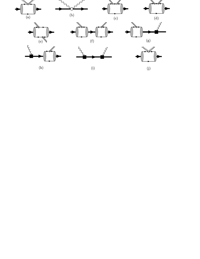
Figure 1: Feynman diagrams for the scalar amplitude of deuteron Compton scattering. The thick initial and final state arrows represent the deuteron. The thick arrows in the middle of the diagrams are the dibaryon states in the ${}^{3}S_{1}$ and ${}^{1}S_{0}$ channels. The open circles denote the electric current interactions, and the shaded circles the magnetic moment interactions. The solid squares are from electromagnetic counter-terms ($L_{1}$ and $L_{2}$). The open square is from the nucleon polarizabilities.

Diagrams contributing to the scalar amplitude $S$ (or equivalently $f_{1}$ and $f_{2}$) to $\mathcal{O}(Q^{2})$ are shown in Fig.1. The gauge-coupling diagrams in 1(a) and 1(b) are of order $Q^{0}$, and of order $Q^{1/2}$ in 1(c). The magnetic diagrams in 1(d) is of order $Q$ and of order $Q^{3/2}$ in 1(e), while those in 1(f)-1(i) are of order $Q^{2}$, with the solid squares denoting magnetic two-body current $L_{1}$ and $L_{2}$. The open square in 1(j) is the nucleon polarizability coupling which also contributes at $Q^{2}$.

The results of the diagrams are expressed in terms of the reduced amplitudes

$$f_{i}=\frac{1}{\left(1-\gamma r^{(^{3}S_{1})}\right)}\widetilde{f}_{i}\ ,$$ (14)

where $i=1-12$. We write

$$\widetilde{f}_{1} = g_{1}(\omega)+g_{1}(-\omega)+zh(\omega)\ ,$$

$$\widetilde{f}_{2} = g_{2}(\omega)+g_{2}(-\omega)-h(\omega)\ ,$$ (15)

where

$$g_{1}(\omega) = \left[\frac{\gamma\,{{\rho}_{d}}}{2}-\frac{4\,\gamma\,}{\sqrt{2-2\,z}\,\omega\,}\tan^{-1}(\frac{\sqrt{2-2\,z}\,\omega}{4\,\gamma})+\frac{2\,\gamma\,\left(\gamma+2\,\sqrt{{\gamma}^{2}-\omega\,{M_{N}-i\varepsilon}}\right)}{3\,{\left(\gamma+\sqrt{{\gamma}^{2}-\omega\,{M_{N}-i\varepsilon}}\right)}^{2}\,}\right.\$$ (16)

$$\left.{+}\frac{32\,\pi\,\gamma\,\omega\,\,{M_{N}}\,{{\alpha}_{0}}}{e^{2}\,\sqrt{2-2\,z}}\tan^{-1}(\frac{\sqrt{2-2\,z}\,\omega}{4\,\gamma})\right]\ ,$$

and

$$h(\omega) = \frac{1\,}{15\,{\omega}^{2}\,{{M_{N}}}^{4}\,}\left(-4\,\gamma\,{\left({\gamma}^{2}-\omega\,{M_{N}-i\varepsilon}\right)}^{\frac{5}{2}}+8\,{\gamma}^{6}+20\,{\gamma}^{4}\,\omega\,{M_{N}}+60\,{\gamma}^{2}\,{\omega}^{2}\,{{M_{N}}}^{2}\right.$$ (17)

$$\left.+15\,{\omega}^{3}\,{{M_{N}}}^{3}-\gamma\,\sqrt{{\gamma}^{2}+\omega\,{M_{N}}}\,\left(4\,{\gamma}^{4}+28\,{\gamma}^{2}\,\omega\,{M_{N}}+39\,{\omega}^{2}\,{{M_{N}}}^{2}\right)\right)\ .$$

and where

$$g_{2}(\omega)=\frac{32\,\pi\,\gamma\,\omega\,\,{M_{N}}\,{{\beta}_{0}}}{e^{2}\,\sqrt{2-2\,z}}\tan^{-1}(\frac{\sqrt{2-2\,z}\,\omega}{4\,\gamma})+\frac{4\,\gamma\,\left(\,\gamma-\sqrt{{\gamma}^{2}-\omega\,{M_{N}-i\varepsilon}}\right)\,{{{\mu}_{1}}}^{2}}{3\,{{M_{N}}}^{2}}+k(\omega)\ ,$$ (18)

and

$$k(\omega)=-\frac{\gamma\,\left[{\omega\,{L_{1}}\,{M_{N}}+2\,\left(\gamma-\sqrt{{\gamma}^{2}-\omega\,{M_{N}-i\varepsilon}}\right)\,{{\mu}_{1}}}\right]^{2}}{3\,{{M_{N}}}^{2}\,\left(\frac{1}{a^{(^{1}S_{0})}}-\sqrt{{\gamma}^{2}-\omega\,{M_{N}-i\varepsilon}}+\frac{r^{(^{1}S_{0})}\,}{2}\left({\gamma}^{2}-\omega\,{M_{N}}\right)\right)}\ .$$ (19)

These results agree with those obtained in the previous calculations dEFT ; rupak . If the effective range is counted as order $Q^{0}$ instead of $Q^{-1}$ then the results of Ref. rupak are reproduced. Also, the results of Ref. dEFT are reproduced up to recoil effects which can be safely neglected.

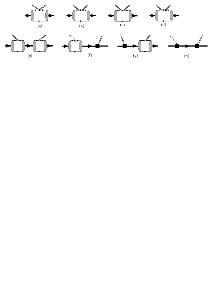
Figure 2: Feynman diagrams for the vector amplitude of deuteron Compton scattering. The solid circles denote the spin-orbit intercation in Eq. (12). Other symbols are the same as described in Fig. 1.

The new contributions we calculate are shown in Fig. 2. Those are diagrams contributing to the vector amplitude $V$ or, equivalently, the amplitudes $f_{3,...,6}$. The solid circle denotes the spin-orbit coupling in Eq. (12). The leading diagrams are 2(a)-2(c) which are of order $Q$. It is interesting to note that the relativistic correction (the spin-orbit interaction in diagram 2(a)) contributes at leading order. Diagram 2(d) is of order $Q^{3/2}$, while diagrams 2(e)-2(h) are of order $Q^{2}$. Naively, if we want to calculate the cross section to order $Q^{2}$, these orders $Q^{3/2}$ and $Q^{2}$ diagrams are not needed according to Eq. (7). We still choose to include these contributions because there is an enhancement factor ${\mu}_{1}^{2}\sim 5.5\sim{1/Q}$ in them. The diagrams give

$$\widetilde{f}_{3} = g_{3}(\omega)-g_{3}(-\omega)+2q(\omega)\ ,$$

$$\widetilde{f}_{4} = g_{4}(\omega)-g_{4}(-\omega)\ ,$$

$$\widetilde{f}_{5} = 0\ ,$$

$$\widetilde{f}_{6} = -q(\omega)\ ,$$ (20)

where

$$g_{3}=\frac{2\,\gamma\left(2\,{{\mu}_{0}}+2\,{{\mu}_{1}-1}\right)}{{M_{N}}}\left[\frac{\,1}{\sqrt{2-2\,z}\,}\tan^{-1}(\frac{\sqrt{2-2\,z}\,\omega}{4\,\gamma})\right]\ .$$ (21)

$$q(\omega) = -\frac{\left({{\mu}_{0}}+{{\mu}_{1}}\right)}{3\,\omega\,{{M_{N}}}^{3}\,\sqrt{{\gamma}^{2}+\omega\,{M_{N}}}}\left[-2\,{\gamma}^{5}+2\,{\gamma}^{3}\,\sqrt{{\gamma}^{2}+\omega\,{M_{N}-i\varepsilon}}\,\left(2\,\gamma-\sqrt{{\gamma}^{2}-\omega\,{M_{N}-i\varepsilon}}\right)\right.$$ (22)

$$+\gamma\,\omega\,{M_{N}}\,\left(-7\,{\gamma}^{2}+3\,\gamma\,\sqrt{{\gamma}^{2}+\omega\,{M_{N}}}+2\,\sqrt{{\gamma}^{4}-\omega^{2}\,{M_{N}^{2}-i\varepsilon}}\,\right)$$

$$\left.+{\omega}^{2}\,{{M_{N}}}^{2}\,\left(-5\,\gamma+3\,\sqrt{{\gamma}^{2}+\omega\,{M_{N}}}\right)\,\right]\ ,$$

and

$$g_{4}(\omega)=\frac{3}{2}k(\omega)-\left({{\mu}_{0}^{2}}+{{\mu}_{1}^{2}}\right)\left[\frac{\omega}{{M_{N}}}+\frac{2\gamma}{{M_{N}^{2}}}\sqrt{{\gamma}^{2}-\omega\,{M_{N}-i\varepsilon}}\right]\ ,$$ (23)

with $k(\omega)$ as given in Eq. (19).

As noted above, the tensor amplitude $T$ only contributes to the cross section at ($Q^{3}$). At the same order, unknown two-body currents $\alpha_{4}$ and $\beta_{4}$ defined in Eq. (13) also contribute. Thus we just calculate the unpolarized Compton scattering to order $Q^{2}$. This will allow us to extract the nucleon electric polarizability $\alpha_{0}$ with $\sim 30\%$ theoretical uncertainty.

Combining the above results, the differential cross section for unpolarized Compton scattering is

$$\left.\frac{d\sigma}{d\Omega}\right|_{cm} = \frac{\alpha^{2}}{6(\omega+2M_{N})^{2}}\text{Re}\left[3(1+z^{2})(f_{1}^{\ast}f_{1}+f_{2}^{\ast}f_{2})+12zf_{1}^{\ast}f_{2}\right.$$ (24)

$$+2(3-z^{2})(f_{3}^{\ast}f_{3}+f_{4}^{\ast}f_{4})+8zf_{3}^{\ast}f_{4}+4(1+3z^{2})(f_{5}^{\ast}f_{5}+f_{6}^{\ast}f_{6})$$

$$+8z(3+z^{2})f_{5}^{\ast}f_{6}+8(1+z^{2})(f_{3}^{\ast}f_{6}+f_{4}^{\ast}f_{5})+16z(f_{3}^{\ast}f_{5}+f_{4}^{\ast}f_{6})]\ ,$$

where $\alpha=1/137$ is the fine structure coupling constant and $z=\cos\theta=\mathbf{\hat{k}}\cdot\mathbf{\hat{k}}^{\prime}.$

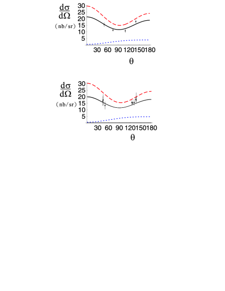
Figure 3: Differential cross section for $\gamma d\rightarrow\gamma d$ with incident photon energy $\omega=49$ MeV (upper plot) and $\omega=$55 MeV (lower plot). The dashed curves are $\mathcal{O}(Q^{2})$ results with no nucleon polarizabilities, $\alpha_{0}=\beta_{0}=0$. The solid curves are results using polarizabilities $\alpha_{0}=10\beta_{0}=1.2\times 10^{-3}$ fm³, calculated in leading order chiral perturbation theory meissner . The dotted curves are the vector amplitudes contributions alone. The 49 MeV data is from Ref. Illinois , while the 55 MeV data is from Ref. Lund .

In Fig. 3, we show the differential cross section for $\omega=49$ MeV (upper plot) and $\omega=$55 MeV (lower plot). The $49$ MeV data is measured at Illinois while the 55 MeV data is actually a superposition of the 54.6, 54.9 and 55.9 MeV data from the Lund experiment. In both plots, the dashed curves are $\mathcal{O}(Q^{2})$ results with no nucleon polarizabilities, $\alpha_{0}=\beta_{0}=0$. The solid curves are results using nucleon polarizabilities calculated in leading order chiral perturbation theory (ChPT) meissner ,

$$\alpha_{0}=10\beta_{0}=\frac{5g_{A}^{2}e^{2}}{192\pi^{2}f_{\pi}^{2}m_{\pi}}=1.2\times 10^{-3}\text{ fm}^{3}\ .$$ (25)

The dotted curves are the contributions of the vector amplitudes which were not included in the previous calculations chen2 ; dEFT ; rupak . These effects are $\sim$20% and are as large as the nucleon polarizability contributions in the backward angles.

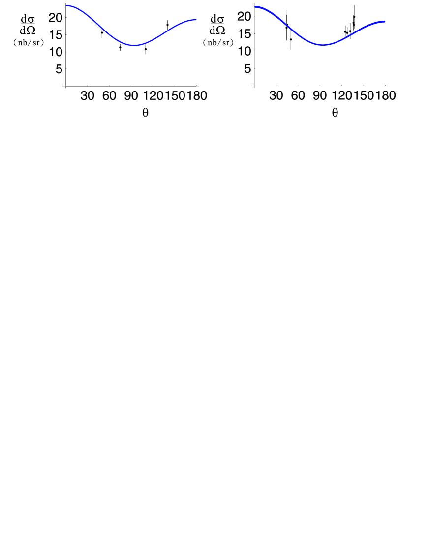
Figure 4: Differential cross section for $\gamma d\rightarrow\gamma d$ with incident photon energy $\omega=49$ MeV (left plot) and $\omega=$55 MeV (right plot). The leading-order ChPT values $\alpha_{0}=10\beta_{0}=1.2\times 10^{-3}$ fm³ are used and the effective range parameter is treated as order $Q^{0}$.

In Fig. 4 we plot the cross section using the counting employed in Ref. rupak and the value of Eq. (25). We set $1/a^{(i)}\sim\omega\sim Q$, $r^{(i)}\sim Q^{0}$ (such that the effective range contributions are treated perturbatively) and expand our amplitudes in $Q$. The leading order ChPT value of nucleon polarizabilities also gives a good description of data. Setting the vector amplitude to be zero, our result coincides with that of Fig. 2 of Ref. rupak .

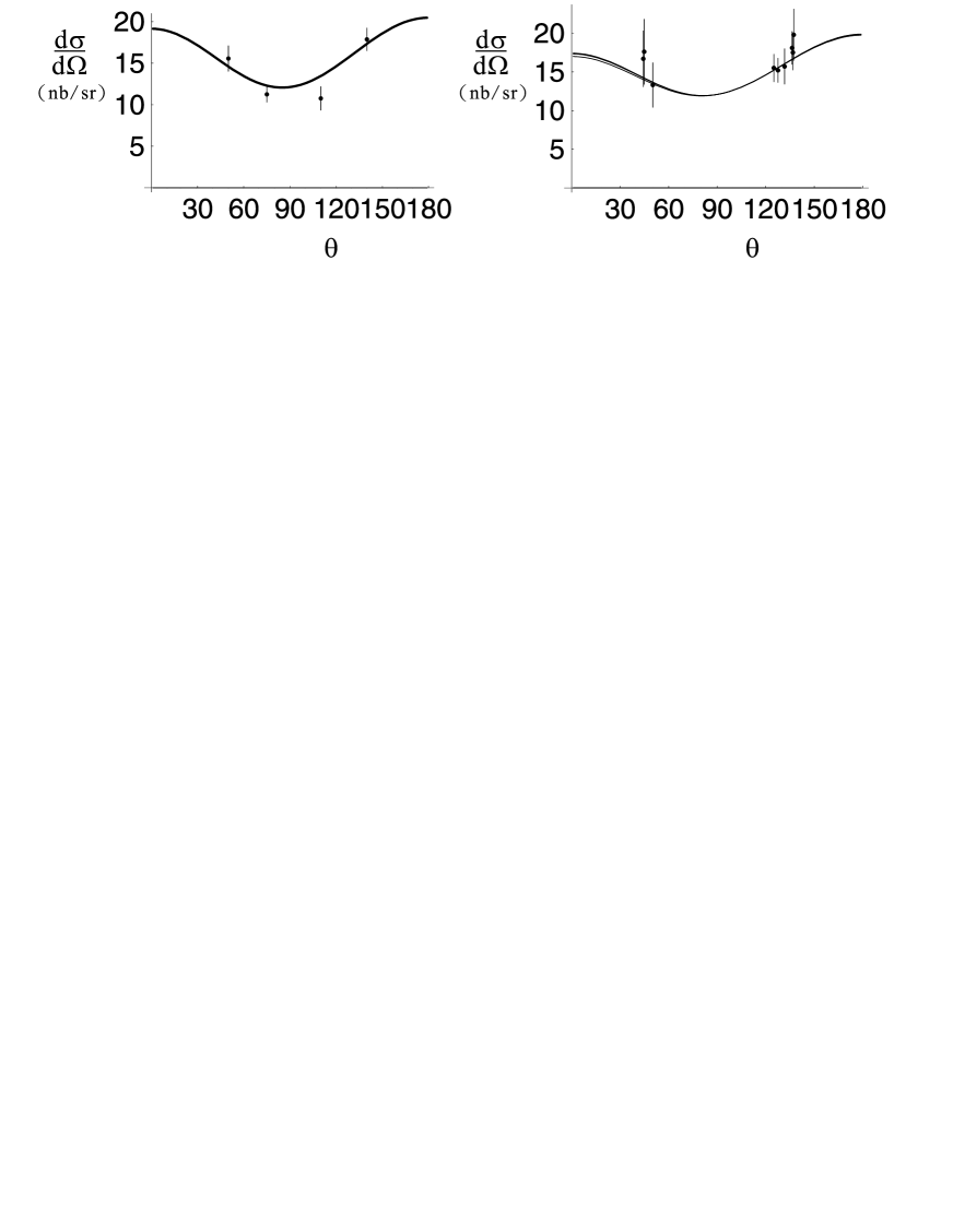
Figure 5: Differential cross section for $\gamma d\rightarrow\gamma d$ with incident photon energy $\omega=49$ MeV (left plot) and $\omega=$55 MeV (right plot). The best fit value $\alpha_{0}=12.3$ and $\beta_{0}=5.0$ (in units of fm^-4) are used and all data points are assumed to be independent in the fitting.

Assuming the data measured at $\omega=$49, 54.6, 54.9 and 55.9 MeV are independent, a $\chi^{2}$ fit gives $\alpha_{0}=12.3\pm 1.4$ and $\beta_{0}=5.0\pm 1.6$ (note that theoretical uncertainty is not included) in the dibaryon formalism. The best fit curves are plotted in Fig. 5. In the counting that treats the effective range perturbatively, the $\chi^{2}$ fit gives $\alpha_{0}=14.2\pm 2.1$ and $\beta_{0}=9.3\pm 2.5$ (theoretical uncertainty is not included) with very similar curves as those shown in Fig. 5. The difference between these two counting schemes is of higher order, thus it appears that while the fit values of $\alpha_{0}$ are quite close to the one predicted by leading order ChPT, the error on $\beta_{0}$ is quite large using the current data. These results can be compared with $\alpha_{0}=8.4\pm 3.4$ and $\beta_{0}=8.9\pm 4.3$ from Ref. rupak , where the contribution of the vector amplitude has been neglected. Thus the vector amplitude has significant effect on a reliable extraction of $\alpha_{0}$.

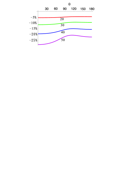
Figure 6: Nucleon polarizability effects on Compton scatterong cross section with $\alpha_{0}=10\beta_{0}=12$ (in units of 10^-4 fm³). The curves, from top to bottom, are for photon energy $\omega=20$, 30, 40 and 50 MeV, respectively.

Future high energy, high precision experiments can take advantage of the theoretically clean pionless EFT by performing the measurement at lower energies. However, the nucleon polarizability contributions become less important at lower energies. To study the best energy range for future experiments, we show the nucleon polarizability effects in the Compton scattering cross section for $\alpha_{0}=10\beta_{0}=12$ (the leading order ChPT value) in Fig. 6. The curves, from top to bottom, are for photon energy $\omega=20$, 30, 40 and 50 MeV, respectively. Given the unknown $\mathcal{O}(Q^{5/2})$ effect is about 5% for a series with expansion parameter $\sim 1/3$ and the theory converges better at $\lesssim$30 MeV, we recommend the best energy range to perform the deuteron Compton measurement is 25-35 MeV. From this figure, we see that a measurement at 30 MeV with 3% error will constrain $\alpha_{0}$ with $3\times 10^{-4}$ fm³ experimental error, which is comparable to the expected theoretical error.

IV Conclusion

We have computed the unpolarized Compton scattering in dibaryon effective field theory at $\mathcal{O}(Q^{2})$. The vector amplitude, which contributes to the cross section at $\mathcal{O}(Q^{2})$ but was not included in previous pionless EFT calculations, was found to affect the extraction of nucleon electric polarizability by more than $50\%$ at 49 MeV. We recommend future high precision deuteron Compton scattering experiments be measured at 25-35 MeV photon energy for appreciable nucleon polarizability effects and controllable theoretical higher-order effects. More specifically, a measurement at 30 MeV with 3% error will constrain $\alpha_{0}$ with $3\times 10^{-4}$ fm³ experimental error, which is comparable to the expected theoretical error.

This work was supported by the U. S. Department of Energy via grant DE-FG02-93ER-40762 and by the National Science Council of Taiwan, ROC. JWC thanks Paulo Bedaque for organizing the Summer of Lattice Workshop 2004 at Lawrence Berkeley Laboratory where part of this research was completed.

References

• (1) P.S. Baranov et al., Sov. J. Nucl. Phys. 21, 355 (1975); A. Ziegler et al., Phys. Lett. B 278, 34 (1992); F.J. Federspiel et al., Phys. Rev. Lett. 67, 1511 (1991); E.L. Hallin et al., Phys. Rev. C 48, 1497 (1993); B.E. MacGibbon et al., Phys. Rev. C 52, 2097 (1995).
• (2) V. Olmos de León et al., Eur. Phys. J. A 10, 207 (2001).
• (3) S.R. Beane, M. Malheiro, J.A. McGovern, D.R. Phillips, U. van Kolck, nucl-th/0403088; Phys. Lett. B567, 200 (2003); Nucl. Phys. A656, 367 (1999).
• (4) Yu.A. Aleksandrov, Phys. Part. Nucl. 32, 708 (2001).
• (5) J. Schmiedmayer et al., Phys. Rev. Lett. 66, 1015 (1991).
• (6) L. Koester et al., Phys. Rev. C 51, 3363 (1995).
• (7) T.L. Enik et al., Sov. J. Nucl. Phys. 60, 567 (1997).
• (8) K. Kossert et al., Phys. Rev. Lett. 88, 162301 (2002).
• (9) M.I. Levchuk, A.I. L’vov, and V.A. Petrun’kin, FIAN report No. 86, 1986; Few-Body Syst. 16, 101 (1994).
• (10) M.A. Lucas, Ph.D. thesis, University of Illinois, 1994.
• (11) D.L. Hornidge et al., Phys. Rev. Lett. 84, 2334 (2000).
• (12) M. Lundin et al., Phys. Rev. Lett. 90, 192501 (2003).
• (13) M. Weyrauch, Phys. Rev. C41, 880 (1990).
• (14) T. Wilbois, P. Wilhelm, and H. Arenhovel, Few-Body Systems Suppl. 9, 263 (1995).
• (15) J. J. Karakowski and G. A. Miller, Phys. Rev. C60, 014001(1999).
• (16) M.I. Levchuk and A.I. L’vov, Nucl. Phys. A674, 449 (2000); M.I. Levchuk and A.I. L’vov, Nucl. Phys. A684, 490 (2001).
• (17) S. Weinberg, Phys. Lett. B251, 288(1990); Nucl. Phys. B363 3(1991).
• (18) D. B. Kaplan, M. J. Savage and M.B. Wise, Phys. Lett. B424, 390(1998); D. B. Kaplan, M. J. Savage and M.B. Wise, Nucl. Phys. B534, 329(1998).
• (19) S. R. Beane, P. F. Bedaque, W. C. Haxton, D. R. Philllips, and M. J. Savage, nucl-th/0008064.
• (20) V. Bernard, N. Kaiser and Ulf-G. Meißner, Phys. Rev. Lett. 67, 1515 (1991); Nucl. Phys. B 373, 364 (1992); Phys. Lett. B 319, 269 (1993).
• (21) D. B. Kaplan, Nucl. Phys. B494, 471(1997).
• (22) U. van Kolck, hep-ph/9711222; Nucl. Phys. A645 273 (1999).
• (23) T.D. Cohen, Phys. Rev. C55, 67 (1997); D.R. Phillips and T.D. Cohen, Phys. Lett. B390, 7 (1997); S.R. Beane, T.D. Cohen, and D.R. Phillips, Nucl. Phys. A632, 445 (1998).
• (24) P.F. Bedaque and U. van Kolck, Phys. Lett. B428, 221 (1998).
• (25) J. W. Chen, G. Rupak, and M. J. Savage, Nucl. Phys. A653, 386 (1999).
• (26) S.R. Beane, P.F. Bedaque, M.J. Savage, and U. van Kolck, Nucl. Phys. A700, 377 (2002).
• (27) J.W. Chen, H.W. Grie$\ss$hammer, M.J. Savage, R.P. Springer, Nucl. Phys. A644, 245(1998); J.W. Chen, Nucl. Phys. A653, 375(1999).
• (28) S. R. Beane and M. J. Savage, Nucl. Phys. A694, 511 (2001).
• (29) H. W. Grie$\ss$hammer and G. Rupak, Phys. Lett. B529, 57 (2002).
• (30) J.W. Chen and M.J. Savage, Phys. Rev. C60, 065205 (1999).
• (31) J.W. Chen, Y. Li and X. Ji, in preparation.