Self-Consistent Description of Multipole Strength in Exotic Nuclei I: Method

Abstract

We use the canonical Hartree-Fock-Bogoliubov basis to implement a completely self-consistent quasiparticle-random-phase approximation with arbitrary Skyrme energy density functionals and density-dependent pairing functionals. The point of the approach is to accurately describe multipole strength functions in spherical even-even nuclei, including weakly-bound drip-line systems. We describe the method and carefully test its accuracy, particularly in handling spurious modes. To illustrate our approach, we calculate isoscalar and isovector monopole, dipole, and quadrupole strength functions in several Sn isotopes, both in the stable region and at the drip lines.

I Introduction

The study of nuclei far from stability is an increasingly important part of nuclear physics NSA ; NUP . As radioactive beams allow more experiments on these nuclei, theoretical modeling is changing in significant ways. New ideas and progress in computer technology have allowed nuclear theorists to understand bits and pieces of nuclear structure quantitatively Carlson et al. . Short-lived exotic nuclei offer unique tests of those aspects of our developing many-body theories that depend on neutron excess Dobaczewski and Nazarewicz (1998). The major challenge is to predict or describe in detail exotic new properties of nuclei far from the stability valley, and to understand the origins of these properties.

For medium-mass and heavy nuclei, an important goal is obtaining a universal energy-density functional, which will be able to describe static and dynamic properties of finite nuclei and extended nucleonic matter with arbitrary neutron-to-proton ratio. Self-consistent methods based on density-functional theory are already sophisticated enough to allow precise analysis of ground-state properties (e.g. binding energies) in heavy nuclei Goriely et al. (2002, 2003); Stoitsov et al. (2003). They can also help describe nuclear decays and excited states. Their predictions for collective excitations as we approach the neutron drip line are especially interesting. What happens to low- and high-frequency multipole modes when the neutron excess is unusually large?

To address these questions we use the quasiparticle random-phase approximation (QRPA), a powerful tool for understanding both low-lying vibrational states and giant resonances Ring and Schuck (1980). The QRPA is a microscopic approach that is nevertheless simple enough to allow “no-core” calculations. The approximation, which should be good for collective vibrations as long as their amplitudes are small, is especially effective in conjunction with Skyrme energy functionals. Our work is a part of a broad program to test and improve these functionals, which thus far have been fitted mainly to ground-state observables, by applying them to collective excitations, particularly near the drip line. This paper lays out our approach and evaluates its accuracy. For these purposes we restrict ourselves to a single Skyrme functional, SkM^∗. A forthcoming study will examine the performance of Skyrme functionals more generally.

The QRPA is a standard method for describing collective excitations in open-shell superconducting nuclei with stable mean-field solutions, either spherical or deformed. What is not standard, and at the same time is extremely important for weakly bound nuclei, is the treatment of the particle continuum. Continuum extensions of the random phase approximation (RPA) or QRPA are usually carried out in coordinate space, facilitating treatment of decay channels and guaranteeing correct asymptotics. Surprisingly, as we discuss below, the rich literature on the RPA and QRPA, which includes many coordinate-space calculations, contains few treatments of the continuum that exploit the entire Skyrme functional in a fully self-consistent way.

To avoid confusion, we state what we mean by a fully self-consistent RPA or QRPA calculation. First, the underlying mean-field calculation must be self-consistent in the usual sense. Next, the residual interaction used in the RPA or QRPA must be derived from the same force or energy functional that determines the mean field. An important consequence of this condition, and of other more detailed technical conditions discussed below, is that spurious excitations arising from symmetry breaking by the mean field have zero or nearly zero energy, leaving the physical intrinsic excitations completely uncontaminated by spurious motion. Finally, energy-weighted sum rules must be satisfied to high accuracy. We elaborate on these requirements below; Refs. Shlomo and Sanzhur (2002); Agrawal et al. (2003); Agrawal and Shlomo discuss ways in which RPA calculations commonly violate them.

The literature applying RPA or QRPA to nuclear structure is huge, and a complete review is beyond the scope of our paper. We do, however, present an overview of the studies that are related in one way or another to nuclear density functionals, self consistency, pairing, and the key issue of the particle continuum.

The standard version of QRPA, the so-called matrix formulation, is carried out in the configuration space Rowe (1970); Waroquier et al. (1987) of single-quasiparticle states. A number of papers treat collective states in spherical nuclei in the Skyrme-RPA and QRPA matrix formulation (see Refs. Waroquier et al. (1987); Colò et al. (2003) and references cited therein), in which the positive-energy continuum is discretized, e.g. by solving the Hartree-Fock-Bogoliubov (HFB) and QRPA equations in a harmonic-oscillator single-particle basis. Within this group, the first fully self-consistent calculations that properly account for continuum effects are those of Refs. Engel et al. (1999); Bender et al. (2002), in which the localized canonical basis of coordinate-space HFB is used to calculate beta-decay rates of neutron-rich r-process nuclei and Gamow-Teller strength distributions. Recently, fully self-consistent HFB+QRPA calculations have also been carried out with the finite-range Gogny force Giambrone et al. (2003). Unlike many previous Gogny+HFB studies that employed a harmonic oscillator basis, Ref. Giambrone et al. (2003) solves the HFB equations in the eigenbasis of a Woods-Saxon potential, the particle continuum of which is discretized by enclosing the system in a box.

Coordinate-space Green’s functions as a method of implementing the RPA through linear response were first used in Ref. Shlomo and Bertsch (1975) and subsequently applied to the description of low- and high-energy nuclear modes (see, e.g., Refs. Liu and Giai (1976); Touv et al. (1980); Hamamoto et al. (1997, 1998); Hamamoto and Sagawa (1999, 2000); Kolomiets et al. (2000); Sagawa (2002); Hamamoto and Sagawa (2002); Shlomo and Sanzhur (2002); Shlomo and Agrawal (2003)). Many of those calculations are not realistic enough, however, because they ignore the spin-orbit and Coulomb residual interactions in the RPA Agrawal et al. (2003); Agrawal and Shlomo . Coordinate-space Green’s-function QRPA was studied in Ref. Hagino and Sagawa (2001), in the BCS approximation, with a phenomenological Woods-Saxon average potential. Coordinate-space HFB+QRPA for spherical nuclei was formulated in Refs. Matsuo (2001, 2002); Khan et al. (2002, 2004) and applied to excitations of neutron-rich nuclei. As in Hagino and Sagawa (2001), the Hartree-Fock (HF) field in Refs. Matsuo (2001, 2002) was approximated by a Woods-Saxon potential. While the calculations of Refs. Khan et al. (2002, 2004) are based on Skyrme-HFB fields, they violate full self consistency by replacing the residual velocity-dependent terms of the Skyrme force by the Landau-Migdal force in the QRPA, and neglecting spin-spin, spin-orbit, and Coulomb residual interactions entirely. Within this approach, extensive Skyrme-HF+BCS QRPA calculations of E1-strength in neutron-rich nuclei were carried out in Refs. Goriely and Khan (2002); Goriely et al. (2004).

An alternative coordinate-representation approach, also based on Green’s functions, was formulated in Refs. Platonov and Saperstein (1988); S.Kamerdzhiev et al. (2004) within Migdal’s finite-Fermi-systems theory. Most of practical applications of this method, however, involve approximations that break self consistency in one way or another, including the use of highly truncated pairing spaces, different interactions in HFB and QRPA, and the so-called diagonal pairing approximation Platonov and Saperstein (1988); Fayans et al. (1994); Horen et al. (1996); Borzov et al. (1995, 1996); Kamerdzhiev et al. (1998, 2001); Borzov (2003); Kamerdzhiev and Litvinova (2004). Properties of excited states and strength functions have also been investigated within the relativistic RPA Ring et al. (2001); Vretenar et al. (2001); Ma et al. (2002); Vretenar et al. (2002); Niksić et al. (2002); Ma et al. (2003); Vretenar et al. (2004) or QRPA Paar et al. (2003, 2004). The QRPA work employs the matrix formulation and is fully self-consistent, since it uses the same Lagrangian in the relativistic Hartree-Bogoliubov calculation of the ground state and in the QRPA matrix equations, which are solved in the canonical basis.

At the present, no fully self-consistent continuum HFB+QRPA calculations exist in deformed nuclei. Refs. Nakatsukasa and Yabana (2002, 2004) studied giant resonances in deformed nuclei within time-dependent HF theory, formulated in coordinate space with a complex absorbing boundary condition imposed. Symmetry-unrestricted RPA calculations, with no pairing, were carried out in Ref. Inakura et al. (2004) in a “mixed representation” Imagawa and Hashimoto (2003) on a Cartesian mesh in a box, while Ref. Hagino et al. (2004) contains examples of BCS+QRPA calculations in the single-particle basis of a deformed Woods-Saxon potential.

The work described in this paper is fully self-consistent: among other things we use precisely the same interaction in the HFB and QRPA calculations so as to preserve the small-amplitude limit of time-dependent HFB. We formulate the QRPA in the canonical eigenbasis of the one-body particle-density matrix Dobaczewski et al. (1996) which is calculated in the coordinate representation in a large spherical box. As mentioned above, the canonical basis has been used previously to study $\beta$ decay and Gamow-Teller strength Engel et al. (1999); Bender et al. (2002); its use in charge-conserving modes near the drip line is more challenging, however, because of the existence of spurious states in the monopole and dipole channels. These zero-energy modes can mix with physical states unless the QRPA equations are solved with high accuracy. A less precise implementation of our approach was used to calculate neutrino-nucleus cross sections in ²⁰⁸Pb in Ref. Engel et al. (2003).

This paper is organized as follows. Section II below presents our approach. In Sec. III we check the QRPA solutions carefully, focusing on spurious modes. Section IV contains the main conclusions of our work. Mathematical details are in two appendices, the first of which is on the QRPA equations and the second on calculating the derivatives of the Skyrme functionals that enter the formalism.

II Method

Our first step in the self-consistent treatment of excitations is to solve the spherical HFB equations in coordinate space (without mixing neutron and proton quasiparticle wave functions Perlińska et al. (2004)), with the method developed in Ref. Dobaczewski et al. (1984) (see also Refs. Dobaczewski et al. (1996, 2001); Bennaceur and Dobaczewski (2004)). We can use arbitrary Skyrme functionals in the particle-hole and pairing (particle-particle) channels.

We modify the code used in Refs. Dobaczewski et al. (1984, 1996, 2001) so that it solves the HFB equations with higher accuracy, which we need because the QRPA uses all the single-quasiparticle states produced by the HFB equations, even those that are essentially unoccupied. Our modifications are: (i) the use of quadruple precision (though in solving the QRPA equations we use double precision); (ii) a smaller discretization length (0.05 fm); and (iii) a high quasiparticle-energy cutoff (200 MeV) and a maximum angular momentum $j_{\rm max}$=15/2 ($N\leq 82$) or 21/2 ($N>82$). In a 20 fm box, this cutoff corresponds to 200–300 quasiparticle states for each kind of nucleon. We include all these quasiparticle states in the HFB calculation because a very large energy cutoff is essential for the accuracy of self-consistent QRPA calculations Agrawal et al. (2003). Hence, the effective pairing window in our HFB calculations is also very large, with the pairing functional fitted to experimental pairing gaps extracted as in Ref. Terasaki et al. (2002) from the measured odd-even mass differences in several Sn, Ni, and Ca isotopes.

Next, we construct the canonical basis, the eigenstates of single-particle density matrix $\rho$. To avoid poor accuracy (see Ref. Dobaczewski et al. (1996)) in the wave functions of the nearly empty canonical particle states, we do not diagonalize $\rho$ directly in coordinate space. Instead we construct an intermediate basis by orthonormalizing a set of functions $\{\varphi^{\mu}_{1}({\bm{r}})+\varphi^{\mu}_{2}({\bm{r}})\}$, where $\varphi^{\mu}_{1}({\bm{r}})$ and $\varphi^{\mu}_{2}({\bm{r}})$ are the upper and lower components of the quasiparticle wave function with energy $E_{\mu}$ Dobaczewski et al. (1984). We use the density matrix in coordinate space to calculate the matrix in this basis, which we then diagonalize to obtain the canonical states. The reason for using the sum of $\varphi^{\mu}_{1}({\bm{r}})$ and $\varphi^{\mu}_{2}({\bm{r}})$ is that solutions of the HFB equations expressed in the canonical basis (Eqs. (4.14) of Ref. Dobaczewski et al. (1996)) are, in the new basis, guaranteed to be numerically consistent with those of the original HFB problem. This is because the configuration space is the same in both cases, independent of the pairing cutoff (see Ref. Dobaczewski et al. (a) for a discussion relevant to this point). Without pairing, when either $\varphi^{\mu}_{1}({\bm{r}})$ or $\varphi^{\mu}_{2}({\bm{r}})$ is equal to zero, our method is equivalent to taking a certain number of HF states, including many unoccupied states.

In the canonical basis, the HFB+QRPA equations have a form almost identical to that of the BCS+QRPA approximation, the only difference being the presence of off-diagonal terms in the single-quasiparticle energies. The QRPA+HFB formalism employs more pairing matrix elements than the QRPA+BCS, however.

As noted already, full self consistency requires the use of the same interaction in the QRPA as in the HFB approximation. More specifically, this means that the matrix elements that enter the QRPA equation are related to second derivatives of a mean-field energy functional. We describe the densities and the form of the functional carefully in the appendices. But we must meet other conditions as well for QRPA calculation to be self-consistent. Essentially all the single-particle or quasiparticle states produced by the HFB calculation must be used in the space of two-quasiparticle QRPA excitations. This requirement is rather stringent, so we truncate the two-quasiparticle space at several levels and check for convergence of the QRPA solution. First we omit canonical-basis wave functions that have occupation probabilities $v_{i}^{2}$ less than some small $v_{\rm crit}^{2}$, (or HF energies greater than some $\varepsilon_{\rm crit}$ if there is no pairing). Then we exclude from the QRPA pairs of canonical states for which the occupation probabilities are both larger than $1-v_{\rm crit}^{2}$. This second cut is based on the assumption that two-particle transfer modes are not strongly coupled to particle-hole excitations. In addition, if the factors containing $u_{i}$ and $v_{i}$ in the QRPA equation — see Eqs. (27) and (28) — are very small, in practice smaller than 0.01, then we set the corresponding matrix elements equal to zero. This does not affect the size of the QRPA space, but significantly speeds up the calculations. For good performance we diagonalize QRPA-Hamiltonian matrices of order $20,000\times 20,000$ in neutron-rich Sn isotopes.

Having solved the QRPA equations, we can then calculate the strength function

$$S_{J}(E)=\frac{1}{\pi}\sum_{k}\sum_{M=-J}^{J}\frac{\gamma(E_{k})|\langle k|\hat{F}_{JM}|0\rangle|^{2}}{(E_{k}-E)^{2}+\gamma^{2}(E_{k})},$$ (1)

for the multipole operator $\hat{F}_{JM}$. The smoothing width $\gamma$ is supposed to be large enough to remove spurious oscillations in $S_{J}(E)$ associated with a finite box radius $R_{\rm box}$ Shlomo et al. (1997); Nakatsukasa and Yabana (2002). A reasonable form, based on a single-particle estimate, for the smoothing width (App. B of Ref. Shlomo et al. (1997)), is

$$\gamma(E)=\left\{\begin{array}[]{ll}\frac{\pi}{R_{\rm box}}\sqrt{\frac{\hbar^{2}(E+\lambda_{\rm n})}{2m}},&E\geq-\lambda_{\rm n}\\ 0.1~{}{\rm MeV},&E<-\lambda_{\rm n}\end{array}\right.,$$ (4)

where $\lambda_{\rm n}$ is the neutron Fermi level and $m$ is the nucleon mass. In deriving Eq. (4) we assumed that the single-proton continuum is effectively shifted up several MeV by the Coulomb barrier. In other words, we associate the threshold energy with the neutron Fermi level.

In all the tests below, we use the Skyrme functional SkM^∗ Bartel et al. (1982) and a volume pairing functional Dobaczewski et al. (2002) ($C^{\tilde{\rho}}(\rho_{00})$ a constant in Eq. (45)). The pairing parameter in Eq. (55) is $V_{0}=-77.5$ MeV fm³. Usually we work in a box of radius 20 fm, though we vary this radius below to see its effects. In several tests we examine the weakly bound nucleus ¹⁷⁴Sn, which is very close to the two-neutron drip line. In this system, the protons are unpaired and the neutrons paired (with $\Delta_{\rm n}$=1.016 MeV) in the HFB ground state.

III Accuracy of solutions

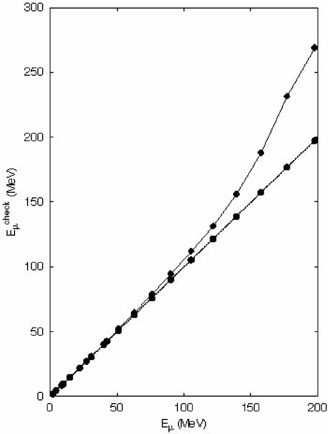
Figure 1: Neutron quasiparticle energies $E_{\mu}^{\rm check}$ for $s_{1/2}$ states in ¹⁷⁴Sn, calculated by diagonalizing the HFB Hamiltonian in the canonical basis, versus the quasiparticle energies $E_{\mu}$ obtained by directly solving the HFB equations in coordinate space. Standard (solid line, diamonds) and improved (dotted line, dots) methods are used to obtain the canonical states. See text for details.

Benchmark tests of the HFB part of our calculations are reported in Ref. Dobaczewski et al. (b). Since the accuracy of the canonical wave functions, in which the QRPA calculations are carried out, strongly affects the quality of results (in particular QRPA self consistency), we take special care to compute them precisely. As discussed in Sec. II, we obtain canonical states by diagonalizing the single-particle density matrix $\rho$ represented in the orthonormalized set of functions $\{\varphi^{\mu}_{1}({\bm{r}})+\varphi^{\mu}_{2}({\bm{r}})\}$. The accuracy of this method is illustrated in Fig. 1, which plots the quasiparticle energies $E_{\mu}^{\rm check}$, obtained by diagonalizing the HFB Hamiltonian in the canonical basis (Eq. (4.20) of Ref. Dobaczewski et al. (1996)), versus the quasiparticle energies $E_{\mu}$ obtained by solving the HFB differential equations directly in coordinate space (Eq. (4.10) of Ref. Dobaczewski et al. (1996)). Two sets of canonical states are used: (i) those obtained through the procedure outlined above (dotted line) and (ii) those obtained in the standard way by diagonalizing the density matrix $\rho(\bm{r},\bm{r}^{\prime})$ in discretized coordinate space (Eq. (3.24a) of Ref. Dobaczewski et al. (1996); solid line). If the canonical basis is precisely determined, $E_{\mu}^{\rm check}$=$E_{\mu}$ and the two sets of $E_{\mu}^{\rm check}$ coincide. Within the standard approach, however, the high canonical energies deviate visibly from their HFB counterparts, i.e., the accuracy of the underlying canonical wave functions is poor. On the other hand, the quasiparticle energies and canonical wave functions calculated within the modified approach introduced above are as accurate as the original solutions to the HFB equations, even for high-lying nearly-empty states. (See also Sec. VI.D of Ref. Tajima (2004) for a discussion relevant to this point.)

Having examined the canonical basis, we turn to the accuracy of the QRPA part of the calculation. To test it, we first consider solutions related to symmetries. If a Hamiltonian is invariant under a symmetry operator $\hat{P}$ and the HFB state $|\Psi\rangle$ spontaneously breaks the symmetry, then $e^{i\alpha\hat{P}}|\Psi\rangle$, with $\alpha$ an arbitrary c-number, is degenerate with the state $|\Psi\rangle$. The QRPA equations have a spurious solution at zero energy associated with the symmetry breaking Ring and Schuck (1980); Blaizot and Ripka (1986), while all other solutions are free of the spurious motion. This property is important for strength functions, and gives us a way of testing the calculations. Since our QRPA equations, which assume spherical symmetry, are based on mean fields that include pairing and are localized in space, there appear spurious states associated with particle-number nonconservation (proton and/or neutron; 0⁺ channel) and center-of-mass motion (1^- channel). These two cases are discussed below in Sec. III.1 and Sec. III.2.

Table 1: The lowest-energy excited $0^{+}$ states in ¹⁷⁴Sn. The second column shows the excitation energies and the third column the squared matrix elements of the particle-number operator between the $k$th excited state and the ground state ($k$=0).

k	$E_{k}$ (MeV)	$|\langle k|\hat{N}|0\rangle|^{2}$
1	0.171	0.120
2	2.833	$0.533\times 10^{-5}$
3	3.090	$0.877\times 10^{-7}$
4	3.810	$0.252\times 10^{-5}$
5	3.878	$0.480\times 10^{-5}$

III.1 The 0⁺ isoscalar mode

In addition to the spurious state associated with nonconservation of particle-number by the HFB, the $0^{+}$ channel contains the important “breathing mode”. In Table 1 we display results from a run with $v^{2}_{\rm crit}$=$10^{-12}$ for neutrons and $\varepsilon_{\rm crit}=150$ MeV for protons, resulting in the inclusion of 310 proton quasiparticle states and the same number of neutron states, with angular momentum up to $j=21/2$. The Table shows the QRPA energies and transition matrix elements of the particle-number operator. The spurious state is below 200 keV, well separated from the other states, all of which have negligible “number-strength”. The nonzero number strength in the spurious state, like the nonzero energy of that state, is a measure of numerical error. If the space of two-quasiparticle states is smaller, with $\varepsilon_{\rm crit}=100$ MeV and $v^{2}_{\rm crit}=10^{-8}$, the energy of the spurious state and the number strength barely change.

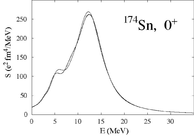
Figure 2: Isoscalar $0^{+}$ strength function in ¹⁷⁴Sn for (i) the single-proton energy cutoff $\varepsilon_{\rm crit}$=100 MeV and the neutron-quasiparticle occupation cutoff $v^{2}_{\rm crit}=10^{-8}$ (thin solid line); (ii) $\varepsilon_{\rm crit}$=150 MeV and $v^{2}_{\rm crit}=10^{-12}$ (dotted line); and (iii) $\varepsilon_{\rm crit}$=200 MeV and $v^{2}_{\rm crit}=10^{-16}$ (thick solid line). Results corresponding to (ii) and (iii) practically coincide.

Figure 2 shows the strength function $S_{J}(E)$ for the isoscalar $0^{+}$ transition operator, cf. Harakeh and van der Woude (2001),

$$\hat{F}_{00}=\frac{eZ}{A}\sum_{i=1}^{A}r_{i}^{2}.$$ (5)

We have plotted three curves with successively more quasiparticle levels (from 246 proton levels and 203 neutron levels to 341 proton levels and 374 neutron levels), with cutoff parameters given in the figure caption. The major structures in the strength function are stable. The error remaining after to the gentlest truncation is extremely small.

The dependence of the strength function on the box size and quasiparticle cutoff is shown in Fig. 3. The upper part of the Figure (panels a-c) corresponds to a constant smoothing width of $\gamma$=0.5 MeV. This relatively small value is not sufficient to eliminate the finite-box effects but it allows us to assess the stability of the QRPA solutions as a function of $R_{\rm box}$. The large structure corresponding to the giant monopole resonance (GMR) is independent of box size no matter what the cutoff, but increasing the number of configurations magnifies the dependence on box size of local fluctuations in $S_{J}(E)$. The lower part of the Figure (panels d-f) are smoothed more realistically, as in Eq. (4). It is gratifying to see that the resulting strength functions are practically identical, i.e., the remaining dependence on $R_{\rm box}$ and the cutoff is very weak.

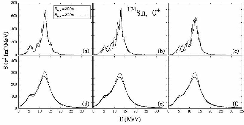
Figure 3: Isoscalar $0^{+}$ strength function in ¹⁷⁴Sn for the box radii: $R_{\rm box}$=20 fm (solid line) and $R_{\rm box}$=25 fm (dotted line). In (a), (b), and (c) the smoothing-width parameter $\gamma$ is 0.5 MeV for all energies, while in (d), (e), and (f) $\gamma(E)$ is given by Eq. (4). We use the same three sets of cutoff conditions as in Fig. 2, namely (i) in parts (a) and (d), (ii) in parts (b) and (e), and (iii) in parts (c) and (f).

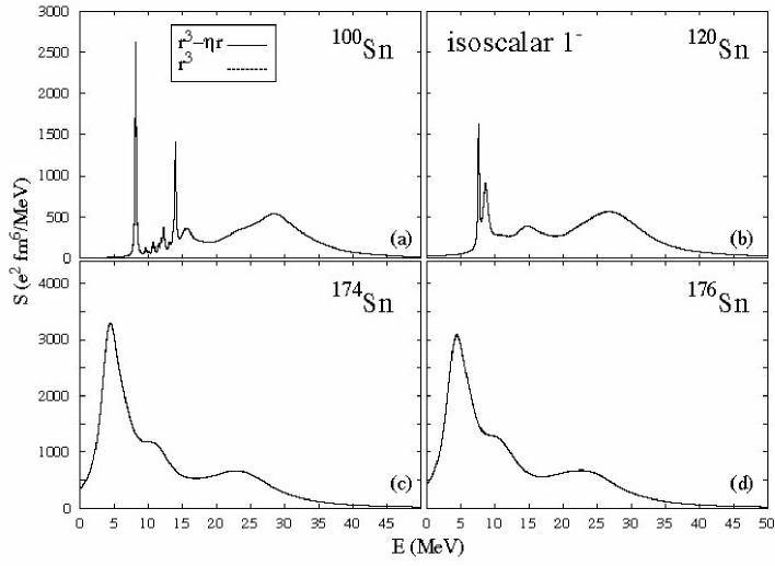
Figure 4: Isoscalar $1^{-}$ strength function in ^{100,120,174,176}Sn for the corrected dipole operator in Eq. (8) (solid line) and the uncorrected operator in Eq. (7) (dotted line). The cutoff $\varepsilon_{\rm crit}$ is 140 MeV and $v^{2}_{\rm crit}$ is $3\times 10^{-12}$. The self consistency of our calculations makes the solid and dotted curves coincide nearly exactly over the whole energy range.

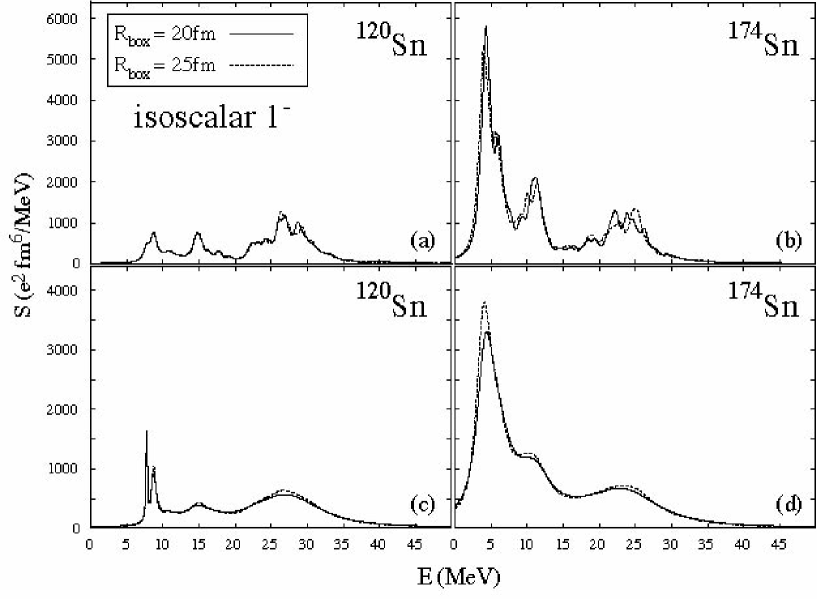
Figure 5: Isoscalar $1^{-}$ strength function in ¹²⁰Sn (left) and ¹⁷⁴Sn (right) for two box radii: $R_{\rm box}$=20 fm (solid line) and $R_{\rm box}$=25 fm (dotted line). In (a) and (b) the smoothing-width parameter is constant ($\gamma$=0.5 MeV), while in (c) and (d) $\gamma(E)$ is given by Eq. (4).

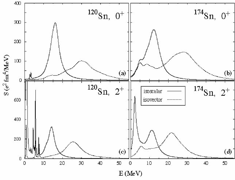
Figure 6: Isoscalar and isovector strength functions for (a) the 0⁺ channel of ¹²⁰Sn, (b) the 0⁺ channel of ¹⁷⁴Sn, (c) the 2⁺ channel of ¹²⁰Sn, and (d) the 2⁺ channel of ¹⁷⁴Sn. The cutoff $\epsilon_{\rm crit}$ is 150 MeV and $v^{2}_{\rm crit}$ is $10^{-12}$.

The energy-weighted sum rule (EWSR) for the isoscalar $0^{+}$ mode Harakeh and van der Woude (2001) is given by

$$\sum_{k}E_{k}|\langle k|\hat{F}_{00}|0\rangle|^{2}=2\frac{e^{2}\hbar^{2}}{m}\frac{Z^{2}}{A}\langle r^{2}\rangle,$$ (6)

where the expectation value is evaluated in the HFB ground state. This sum rule provides a stringent test of self consistency in the QRPA. In ¹⁷⁴Sn, the right-hand side of Eq. (6) is 35215 $e^{2}$ MeV fm⁴ and the left-hand side 34985$\pm 15$ $e^{2}$ MeV fm⁴ for all of the calculations of Fig. 3; the QRPA strength essentially exhausts the sum rule. (The QRPA values of the EWSR in this paper are obtained by summing up to $E_{k}=50$ MeV. )

III.2 The isoscalar 1^- mode

The $1^{-}$ channel, home of the giant dipole resonance, the isoscalar squeezing resonance, and as yet incompletely understood low-energy peaks in neutron-rich nuclei (sometimes associated with skin excitations), has a spurious isoscalar mode associated with center-of-mass motion that can seriously compromise the low-energy spectrum if not handled with extreme care. We test the ability of our QRPA to do so in ¹⁰⁰Sn, ¹²⁰Sn, ¹⁷⁴Sn, and ¹⁷⁶Sn. (The nuclei ¹⁰⁰Sn and ¹⁷⁶Sn are the two-proton and two-neutron drip-line systems predicted by the HFB calculation with SkM^∗. Neither nucleus has any static pairing, i.e., $\Delta_{\rm n}$=$\Delta_{\rm p}$=0.) In the following calculations, we take $\varepsilon_{\rm crit}=140$ MeV for the protons and $v^{2}_{\rm crit}=9\times 10^{-12}$ for the neutrons. As discussed above, smoothed strength functions are practically independent of small changes in the cutoff. They are also independent of the cutoff in quasiparticle angular momentum provided we include all states with $j$$\leq$15/2.

Figure 4 shows the predicted isoscalar dipole strength function for ^{100,120,174,176}Sn. For the transition operator, we use

$$\hat{F}_{1M}=\frac{eZ}{A}\sum_{i=1}^{A}r_{i}^{3}Y_{1M}(\Omega_{i})~{},$$ (7)

and the corrected operator

$$\hat{F}_{1M}^{\rm cor}=\frac{eZ}{A}\sum_{i=1}^{A}(r_{i}^{3}-\eta r_{i})Y_{1M}(\Omega_{i}),\ \ \eta=\frac{5}{3}\langle r^{2}\rangle,$$ (8)

to remove as completely as possible residual pieces of the spurious state from the physical states Agrawal et al. (2003). The fact that the strength functions produced by these two operators — displayed in Fig. 4 — coincide so closely shows the extreme accuracy of our QRPA solutions; they are uncontaminated by spurious motion even without the operator correction. The spurious-state energies $E_{\rm spurious}$ are 0.964 MeV for ¹⁰⁰Sn and 0.713 MeV for ¹²⁰Sn, and the energies of the first physical excited states are 7.958 MeV for ¹⁰⁰Sn and 7.729 MeV for ¹²⁰Sn. In ¹⁷⁴Sn (¹⁷⁶Sn), $E_{\rm spurious}$ is 0.319 MeV (0.349 MeV) and the first physical state is at 3.485 MeV (2.710 MeV), lower than in the more stable isotopes. Pairing correlations do not affect accuracy; the neutrons in ¹²⁰Sn and ¹⁷⁴Sn are paired, while those in ¹⁰⁰Sn and ¹⁷⁶Sn are not.

We display the fine structure of the isoscalar $1^{-}$ strength functions in ¹²⁰Sn and ¹⁷⁴Sn in Fig. 5, which also illustrates the dependence of the results on $R_{\rm box}$. The dependence is consistent with that of Fig. 3 for the isoscalar 0⁺ strength; the low-amplitude fluctuations in $S_{J}(E)$ that are unstable as a function of $R_{\rm box}$ disappear, and the smoothed strength function depends only weakly on $R_{\rm box}$. In ¹²⁰Sn, the two sharp peaks below 10 MeV correspond to discrete states while the broad maxima centered around 15 MeV and 27 MeV are in the continuum, well above neutron-emission threshold. A similar three-peaked structure emerges in ¹⁷⁴Sn, though most of the strength there is concentrated in the low-energy peak at $E\approx 4$ MeV. Fig. 4 shows (as we will discuss in our forthcoming paper J. Terasaki et al., in preparation () (2004)) that the appearance of the low-energy isoscalar dipole strength is a real and dramatic feature of neutron-rich dripline nuclei Catara et al. (1997); Sagawa and Esbensen (2001). The EWSR for the isoscalar $1^{-}$ mode Harakeh and van der Woude (2001) is

$$\sum_{k}\sum_{M}E_{k}|\langle k|\hat{F}_{1M}^{\rm cor}|0\rangle|^{2}=\frac{3}{8\pi}\frac{e^{2}\hbar^{2}}{m}\frac{Z^{2}}{A}\left(11\langle r^{4}\rangle-\frac{25}{3}\langle r^{2}\rangle^{2}\right).$$ (9)

In ¹⁷⁴Sn, the right-hand side is 403310 $e^{2}$ MeV fm⁶, while the left-hand side is 400200 $e^{2}$ MeV fm⁶. For ¹⁷⁶Sn, the corresponding numbers are 406576 $e^{2}$ MeV fm⁶ and 407100 $e^{2}$ MeV fm⁶. This level of agreement is very good.

III.3 The isovector 0⁺ and isoscalar, isovector 2⁺ modes

Figure 6 displays strength functions for the 0⁺ and 2⁺ channels in ¹²⁰Sn and ¹⁷⁴Sn. (We discussed the isoscalar $0^{+}$ mode above to illustrate the accuracy of our solutions, but include it here as well for completeness.) The calculations show the appearance of low-energy $0^{+}$ strength — both isovector and isoscalar — and low-energy isovector 2⁺ strength in ¹⁷⁴Sn, though in none of these instances is the phenomenon quite as dramatic as in the isoscalar $1^{-}$ channel.

The EWSR for the isoscalar 2⁺ transition operator,

$$\hat{F}_{2M}=e{\frac{Z}{A}}\sum_{i=1}^{A}r_{i}^{2}Y_{2M}(\Omega_{i}),$$ (10)

can be written as Harakeh and van der Woude (2001)

$$\sum_{k}\sum_{M}E_{k}|\langle k|\hat{F}_{2M}|0\rangle|^{2}=\frac{25}{4\pi}\frac{e^{2}\hbar^{2}}{m}\frac{Z^{2}}{A}\langle r^{2}\rangle.$$ (11)

The sum rule is obeyed as well in the 2⁺ isoscalar channel as in the $0^{+}$ and $1^{-}$ channels, the only difference being that one needs to include quasiparticle states with $j>15/2$ for ¹⁷⁴Sn. For ¹²⁰Sn (¹⁷⁴Sn) from Fig. 6, the EWSR is 37222 (34971) $e^{2}$ MeV fm⁴ while the QRPA value is 37030 (35010) $e^{2}$ MeV fm⁴.

While on the topic of the sum rule, we display in Table 2 the $j_{\rm max}$-dependence of the EWSR for several channels in ¹⁵⁰Sn, with $R_{\rm box}=25$ fm. By taking $j_{\rm max}=19/2$ we appear to obtain essentially the entire strength in all three cases.

Table 2: The $j_{\rm max}$-dependence of isoscalar EWSR for ¹⁵⁰Sn. $R_{\rm box}$ is 25 fm.

$T$ $J^{\pi}$	units	$j_{\rm max}=19/2$	$j_{\rm max}=25/2$
IS 0+	$(e^{2}~{}{\rm MeV}~{}{\rm fm}^{4})$	35731	35633
IS 1-	$(e^{2}~{}{\rm MeV}~{}{\rm fm}^{6})$	361686	353936
IS 2+	$(e^{2}~{}{\rm MeV}~{}{\rm fm}^{4})$	35542	35445

IV Conclusion

In this work we have reported on the development and detailed testing of a fully self-consistent Skyrme-QRPA framework that employs the canonical HFB basis. The method can be used to calculate strength distributions in any spin-isospin channel and in any spherical even-even nucleus. A good calculation requires a large single-quasiparticle space. Our results show that our space is large enough in nuclei as heavy as the Sn isotopes.

We are currently investigating the predictions of a range of Skyrme functionals across the Ca, Ni, and Sn isotope chains. The initial results presented here point to increases in low-lying strength at the neutron drip line, particularly in the isoscalar-dipole channel. In a forthcoming paper J. Terasaki et al., in preparation () (2004) we will report on the robustness of these effects, on the physics underlying them, on their variation with atomic mass and number, and on their implications for the future of Skyrme functionals.

Appendix A QRPA equation

The QRPA equations are the small-oscillations limit of the time-dependent Hartree-Fock-Bogoliubov approximation, see, e.g., Ring and Schuck (1980); Waroquier et al. (1987). In the canonical basis the most general equations take the form

$$\sum_{L<L^{\prime}}\left(\begin{array}[]{cc}A_{KK^{\prime},LL^{\prime}}&B_{KK^{\prime},LL^{\prime}}\\ -B^{\ast}_{KK^{\prime},LL^{\prime}}&-A^{\ast}_{KK^{\prime},LL^{\prime}}\end{array}\right)\left(\begin{array}[]{c}{X}^{k}_{LL^{\prime}}\\ {Y}^{k}_{LL^{\prime}}\end{array}\right)=E_{k}\left(\begin{array}[]{c}{X}^{k}_{KK^{\prime}}\\ {Y}^{k}_{KK^{\prime}}\end{array}\right),\ \ K<K^{\prime},$$ (12)

$$A_{KK^{\prime},LL^{\prime}} = E_{KL}\delta_{K^{\prime}L^{\prime}}-E_{K^{\prime}L}\delta_{KL^{\prime}}-E_{KL^{\prime}}\delta_{K^{\prime}L}+E_{K^{\prime}L^{\prime}}\delta_{KL}$$ (13)

$$-\bar{V}^{\rm ph}_{K\bar{L}\bar{K}^{\prime}L^{\prime}}u_{L^{\prime}}v_{L}u_{K}v_{K^{\prime}}+\bar{V}^{\rm ph}_{K^{\prime}\bar{L}\bar{K}L^{\prime}}u_{L^{\prime}}v_{L}u_{K^{\prime}}v_{K}$$

$$+\bar{V}^{\rm ph}_{K\bar{L}^{\prime}\bar{K}^{\prime}L}u_{L}v_{L^{\prime}}u_{K}v_{K^{\prime}}-\bar{V}^{\rm ph}_{K^{\prime}\bar{L}^{\prime}\bar{K}L}u_{L}v_{L^{\prime}}u_{K^{\prime}}v_{K}$$

$$-\bar{V}^{\rm pp}_{\bar{L}\bar{L}^{\prime}\bar{K}^{\prime}\bar{K}}v_{L}v_{L^{\prime}}v_{K^{\prime}}v_{K}-\bar{V}^{\rm pp}_{KK^{\prime}{L}^{\prime}L}u_{K}u_{K^{\prime}}u_{L}u_{L^{\prime}}$$

$$-\bar{V}^{\rm 3p1h}_{\bar{L}\bar{L}^{\prime}{K}\bar{K}^{\prime}}v_{L}v_{L^{\prime}}u_{K}v_{K^{\prime}}+\bar{V}^{\rm 3p1h}_{\bar{L}\bar{L}^{\prime}{K}^{\prime}\bar{K}}v_{L}v_{L^{\prime}}u_{K^{\prime}}v_{K}$$

$$-\bar{V}^{\rm 3p1h}_{{K}{K}^{\prime}\bar{L}{L}^{\prime}}u_{K}u_{K^{\prime}}u_{L^{\prime}}v_{L}+\bar{V}^{\rm 3p1h}_{{K}{K}^{\prime}\bar{L}^{\prime}{L}}u_{K}u_{K^{\prime}}u_{L}v_{L^{\prime}}$$

$$-\bar{V}^{\rm 1p3h}_{\bar{L}{L}^{\prime}\bar{K}^{\prime}\bar{K}}u_{L^{\prime}}v_{L}v_{K^{\prime}}v_{K}+\bar{V}^{\rm 1p3h}_{\bar{L}^{\prime}{L}\bar{K}^{\prime}\bar{K}}u_{L}v_{L^{\prime}}v_{K^{\prime}}v_{K}$$

$$-\bar{V}^{\rm 1p3h}_{{K}\bar{K}^{\prime}{L}^{\prime}{L}}u_{K}v_{K^{\prime}}u_{L}u_{L^{\prime}}+\bar{V}^{\rm 1p3h}_{{K}^{\prime}\bar{K}{L}^{\prime}{L}}u_{K^{\prime}}v_{K}u_{L}u_{L^{\prime}},$$

$$B_{KK^{\prime},LL^{\prime}} = \bar{V}^{\rm ph}_{K^{\prime}L^{\prime}\bar{K}\bar{L}}u_{L^{\prime}}v_{L}u_{K^{\prime}}v_{K}-\bar{V}^{\rm ph}_{KL^{\prime}\bar{K^{\prime}}\bar{L}}u_{L^{\prime}}v_{L}u_{K}v_{K^{\prime}}$$ (14)

$$-\bar{V}^{\rm ph}_{K^{\prime}L\bar{K}\bar{L}^{\prime}}u_{L}v_{L^{\prime}}u_{K^{\prime}}v_{K}+\bar{V}^{\rm ph}_{KL\bar{K}^{\prime}\bar{L}^{\prime}}u_{L}v_{L^{\prime}}u_{K}v_{K^{\prime}}$$

$$+\bar{V}^{\rm pp}_{K^{\prime}{K}\bar{L}\bar{L}^{\prime}}v_{L}v_{L^{\prime}}u_{K}u_{K^{\prime}}+\bar{V}^{\rm pp}_{L^{\prime}{L}\bar{K}\bar{K}^{\prime}}v_{K}v_{K^{\prime}}u_{L}u_{L^{\prime}}$$

$$+\bar{V}^{\rm 3p1h}_{K^{\prime}{K}{L^{\prime}}\bar{L}}u_{L^{\prime}}v_{L}u_{K}u_{K^{\prime}}-\bar{V}^{\rm 3p1h}_{K^{\prime}{K}{L}\bar{L}^{\prime}}u_{L}v_{L^{\prime}}u_{K}u_{K^{\prime}}$$

$$+\bar{V}^{\rm 3p1h}_{L^{\prime}{L}{K^{\prime}}\bar{K}}u_{K^{\prime}}v_{K}u_{L}u_{L^{\prime}}-\bar{V}^{\rm 3p1h}_{L^{\prime}{L}{K}\bar{K}^{\prime}}u_{K}v_{K^{\prime}}u_{L}u_{L^{\prime}}$$

$$+\bar{V}^{\rm 1p3h}_{K^{\prime}\bar{K}\bar{L}\bar{L}^{\prime}}v_{L}v_{L^{\prime}}u_{K^{\prime}}v_{K}-\bar{V}^{\rm 1p3h}_{K\bar{K}^{\prime}\bar{L}\bar{L}^{\prime}}v_{L}v_{L^{\prime}}u_{K}v_{K^{\prime}}$$

$$+\bar{V}^{\rm 1p3h}_{L^{\prime}\bar{L}\bar{K}\bar{K}^{\prime}}v_{K}v_{K^{\prime}}u_{L^{\prime}}v_{L}-\bar{V}^{\rm 1p3h}_{L\bar{L}^{\prime}\bar{K}\bar{K}^{\prime}}v_{K}v_{K^{\prime}}u_{L}v_{L^{\prime}},$$

$$\bar{V}^{\rm ph}_{KLK^{\prime}L^{\prime}}=\frac{\delta^{2}E[\rho,\kappa,\kappa^{\ast}]}{\delta\rho_{K^{\prime}K}\delta\rho_{L^{\prime}L}},$$ (15)

$$\bar{V}^{\rm pp}_{K^{\prime}KL^{\prime}L}=\frac{\delta^{2}E[\rho,\kappa,\kappa^{\ast}]}{\delta\kappa^{\ast}_{K^{\prime}K}\delta\kappa_{L^{\prime}L}},$$ (16)

$$\bar{V}^{\rm 3p1h}_{K^{\prime}KL^{\prime}L}=\frac{\delta^{2}E[\rho,\kappa,\kappa^{\ast}]}{\delta\kappa^{\ast}_{K^{\prime}K}\delta\rho_{LL^{\prime}}}={\bar{V}^{\rm 1p3h\ \ast}}_{LL^{\prime}K^{\prime}K},$$ (17)

where $K$ and $L$ are single-particle indices for the canonical basis, and the states are assumed to be ordered. The symbol $\bar{K}$ refers to the conjugate partner of $K$, $u_{K}$ and $v_{K}$ come from the BCS transformation associated with the canonical basis, and the $E_{KL}$ are the one-quasiparticle matrix elements of the HFB Hamiltonian (cf. Eq. (4.14b) of Ref. Dobaczewski et al. (1996)). $X^{k}_{LL^{\prime}}$ and $Y^{k}_{LL^{\prime}}$ are the forward and backward amplitudes of the QRPA solution $k$, and $E_{k}$ is the corresponding excitation energy. $E[\rho,\kappa,\kappa^{\ast}]$ is the energy functional (see App. B for an explicit definition) and $\rho$ and $\kappa$ are the density matrix and pairing tensor. After taking the functional derivatives, we replace $\rho$ and $\kappa$ by their HFB solutions, in complete analogy with an ordinary Taylor-series expansion.

To write the equations in coupled form, we introduce the notation

$$K\equiv(n_{\mu}l_{\mu}j_{\mu}m_{\mu})\equiv(\mu m_{\mu}),\ \ L\equiv(\nu m_{\nu}),\ \$$ (18)

where $(nljm)$ denote spherical quantum numbers. Using (i) rotational, time-reversal, and parity symmetries of the HFB state, (ii) the conjugate single-particle state

$$|\overline{K}\rangle=|\overline{\mu m_{\mu}}\rangle=(-)^{j_{\mu}-m_{\mu}}|\mu\>-m_{\mu}\rangle,$$ (19)

and (iii) the relations

$$X^{k}_{KK^{\prime}}=\langle j_{\mu}m_{\mu}j_{\mu^{\prime}}m_{\mu^{\prime}}|J_{k}M_{k}\rangle\bar{X}^{k}_{[\mu\mu^{\prime}]J_{k}}\times\left\{\begin{array}[]{cc}\sqrt{2},&\mu=\mu^{\prime},\\ 1,&\mbox{otherwise},\end{array}\right.$$ (22)

$$Y^{k}_{KK^{\prime}}=(-)^{j_{\mu}-m_{\mu}}(-)^{j_{\mu^{\prime}}-m_{\mu^{\prime}}}\langle j_{\mu}-m_{\mu}j_{\mu^{\prime}}-m_{\mu^{\prime}}|J_{k}M_{k}\rangle\bar{Y}^{k}_{[\mu\mu^{\prime}]J_{k}}\times\left\{\begin{array}[]{cc}\sqrt{2},&\mu=\mu^{\prime},\\ 1,&\mbox{otherwise},\end{array}\right.$$ (25)

with $J_{k}$ the angular momentum of the state $k$ and the factor $\sqrt{2}$ for convenience Rowe (1970), one can rewrite the QRPA equation as

$$\sum_{\nu\leq\nu^{\prime}}\left(\begin{array}[]{cc}A_{[\mu\mu^{\prime}]J_{k},[\nu\nu^{\prime}]J_{k}}&B_{[\mu\mu^{\prime}]J_{k},[\bar{\nu}\bar{\nu}^{\prime}]J_{k}}\\ -B^{\ast}_{[\mu\mu^{\prime}]J_{k},[\bar{\nu}\bar{\nu}^{\prime}]J_{k}}&-A^{\ast}_{[\mu\mu^{\prime}]J_{k},[\nu\nu^{\prime}]J_{k}}\end{array}\right)\left(\begin{array}[]{c}\bar{X}^{k}_{[\nu\nu^{\prime}]J_{k}}\\ \bar{Y}^{k}_{[\nu\nu^{\prime}]J_{k}}\end{array}\right)=E_{k}\left(\begin{array}[]{c}\bar{X}^{k}_{[\mu\mu^{\prime}]J_{k}}\\ \bar{Y}^{k}_{[\mu\mu^{\prime}]J_{k}}\end{array}\right),\ \ \mu\leq\mu^{\prime},$$ (26)

$$A_{[\mu\mu^{\prime}]J_{k},[\nu\nu^{\prime}]J_{k}} = \frac{1}{\sqrt{1+\delta_{\mu\mu^{\prime}}}}\frac{1}{\sqrt{1+\delta_{\nu\nu^{\prime}}}}\left\{E_{\mu\nu}\>\delta_{\mu^{\prime}\nu^{\prime}}-E_{\mu^{\prime}\nu}\>\delta_{\mu\nu^{\prime}}(-)^{j_{\mu}+j_{\mu^{\prime}}-J_{k}}\right.$$ (27)

$$-E_{\mu\nu^{\prime}}\>\delta_{\mu^{\prime}\nu}(-)^{j_{\mu}+j_{\mu^{\prime}}-J_{k}}+E_{\mu^{\prime}\nu^{\prime}}\>\delta_{\mu\nu}$$

$$+G(\mu\mu^{\prime}\nu\nu^{\prime};J_{k})(u_{\mu^{\prime}}u_{\mu}u_{\nu}u_{\nu^{\prime}}+v_{\nu}v_{\nu^{\prime}}v_{\mu^{\prime}}v_{\mu})$$

$$+F(\mu\mu^{\prime}\nu\nu^{\prime};J_{k})(u_{\mu}v_{\nu^{\prime}}u_{\nu}v_{\mu^{\prime}}+u_{\mu^{\prime}}v_{\nu}u_{\nu^{\prime}}v_{\mu})$$

$$-(-)^{j_{\nu^{\prime}}+j_{\nu}-J_{k}}F(\mu\mu^{\prime}\nu^{\prime}\nu;J_{k})(u_{\mu}v_{\nu}u_{\nu^{\prime}}v_{\mu^{\prime}}+u_{\mu^{\prime}}v_{\nu^{\prime}}u_{\nu}v_{\mu})$$

$$-H(\mu\mu^{\prime}\nu\nu^{\prime};J_{k})(v_{\nu}v_{\nu^{\prime}}u_{\mu}v_{\mu^{\prime}}+u_{\mu^{\prime}}v_{\mu}u_{\nu}u_{\nu^{\prime}})$$

$$+(-)^{j_{\mu}+j_{\mu^{\prime}}-J_{k}}H(\mu^{\prime}\mu\nu\nu^{\prime};J_{k})(v_{\nu}v_{\nu^{\prime}}u_{\mu^{\prime}}v_{\mu}+u_{\mu}v_{\mu^{\prime}}u_{\nu}u_{\nu^{\prime}})$$

$$-H^{\ast}(\nu\nu^{\prime}\mu\mu^{\prime};J_{k})(u_{\mu}u_{\mu^{\prime}}u_{\nu^{\prime}}v_{\nu}+u_{\nu}v_{\nu^{\prime}}v_{\mu^{\prime}}v_{\mu})$$

$$+(-)^{j_{\nu}+j_{\nu^{\prime}}-J_{k}}H^{\ast}(\nu^{\prime}\nu\mu\mu^{\prime};J_{k})(u_{\mu}u_{\mu^{\prime}}u_{\nu}v_{\nu^{\prime}}+u_{\nu^{\prime}}v_{\nu}v_{\mu^{\prime}}v_{\mu})\left.\right\},$$

$$B_{[\mu\mu^{\prime}]J_{k},[\bar{\nu}\bar{\nu}^{\prime}]J_{k}} = \frac{1}{\sqrt{1+\delta_{\mu\mu^{\prime}}}}\frac{1}{\sqrt{1+\delta_{\nu\nu^{\prime}}}}\left\{-G(\mu\mu^{\prime}\nu\nu^{\prime};J_{k})(u_{\mu^{\prime}}u_{\mu}v_{\nu}v_{\nu^{\prime}}+u_{\nu}u_{\nu^{\prime}}v_{\mu^{\prime}}v_{\mu})\right.$$ (28)

$$-(-)^{j_{\nu}+j_{\nu^{\prime}}-J_{k}}F(\mu\mu^{\prime}\nu^{\prime}\nu;J_{k})(u_{\mu}u_{\nu}v_{\mu^{\prime}}v_{\nu^{\prime}}+u_{\mu^{\prime}}u_{\nu^{\prime}}v_{\nu}v_{\mu})$$

$$+(-)^{j_{\nu}+j_{\nu^{\prime}}+j_{\mu}+j_{\mu^{\prime}}}F(\mu^{\prime}\mu\nu^{\prime}\nu;J_{k})(u_{\mu^{\prime}}u_{\nu}v_{\nu^{\prime}}v_{\mu}+u_{\mu}u_{\nu^{\prime}}v_{\mu^{\prime}}v_{\nu})$$

$$+H(\mu\mu^{\prime}\nu\nu^{\prime};J_{k})(v_{\nu}v_{\nu^{\prime}}u_{\mu^{\prime}}v_{\mu}+u_{\mu}v_{\mu^{\prime}}u_{\nu}u_{\nu^{\prime}})$$

$$-(-)^{j_{\mu}+j_{\mu^{\prime}}-J_{k}}H(\mu^{\prime}\mu\nu\nu^{\prime};J_{k})(v_{\nu}v_{\nu^{\prime}}u_{\mu}v_{\mu^{\prime}}+u_{\mu^{\prime}}v_{\mu}u_{\nu}u_{\nu^{\prime}})$$

$$-H^{\ast}(\nu\nu^{\prime}\mu\mu^{\prime};J_{k})(v_{\mu}v_{\mu^{\prime}}u_{\nu^{\prime}}v_{\nu}+u_{\nu}v_{\nu^{\prime}}u_{\mu}u_{\mu^{\prime}})$$

$$+(-)^{j_{\nu}+j_{\nu^{\prime}}-J_{k}}H^{\ast}(\nu^{\prime}\nu\mu\mu^{\prime};J_{k})(v_{\mu}v_{\mu^{\prime}}u_{\nu}v_{\nu^{\prime}}+u_{\nu^{\prime}}v_{\nu}u_{\mu}u_{\mu^{\prime}})\left.\right\},$$

$$G(\mu\mu^{\prime}\nu\nu^{\prime};J_{k}) = \sum_{m_{\mu}m_{\mu^{\prime}}m_{\nu}m_{\nu^{\prime}}}\langle j_{\mu}m_{\mu}j_{\mu^{\prime}}m_{\mu^{\prime}}|J_{k}M_{k}\rangle\langle j_{\nu}m_{\nu}j_{\nu^{\prime}}m_{\nu^{\prime}}|J_{k}M_{k}\rangle\bar{V}^{\rm pp}_{KK^{\prime}LL^{\prime}}$$ (29)

$$\equiv \langle[\mu\mu^{\prime}]J_{k}|\bar{V}^{\rm pp}|[\nu\nu^{\prime}]J_{k}\rangle,$$

$$F(\mu\mu^{\prime}\nu\nu^{\prime};J_{k}) = \sum_{m_{\mu}m_{\mu^{\prime}}m_{\nu}m_{\nu^{\prime}}}\langle j_{\mu}m_{\mu}j_{\mu^{\prime}}m_{\mu^{\prime}}|J_{k}M_{k}\rangle\langle j_{\nu}m_{\nu}j_{\nu^{\prime}}m_{\nu^{\prime}}|J_{k}M_{k}\rangle\bar{V}^{\rm ph}_{K\bar{L^{\prime}}\bar{K^{\prime}}L}$$ (32)

$$= \sum_{J^{\prime}}(-)^{j_{\mu^{\prime}}+j_{\nu}+J^{\prime}}\left\{\begin{array}[]{ccc}j_{\mu}&j_{\mu^{\prime}}&J_{k}\\ j_{\nu}&j_{\nu^{\prime}}&J^{\prime}\end{array}\right\}(2J^{\prime}+1)\langle[\mu\nu^{\prime}]J_{k}|\bar{V}^{\rm ph}|[\mu^{\prime}\nu]J_{k}\rangle,$$

$$H(\mu\mu^{\prime}\nu\nu^{\prime};J_{k}) = \sum_{m_{\mu}m_{\mu^{\prime}}m_{\nu}m_{\nu^{\prime}}}\langle j_{\mu}m_{\mu}j_{\mu^{\prime}}m_{\mu^{\prime}}|JM\rangle\langle j_{\nu}m_{\nu}j_{\nu^{\prime}}m_{\nu^{\prime}}|JM\rangle\bar{V}^{\rm 3p1h}_{\bar{L}\bar{L}^{\prime}K\bar{K}^{\prime}}$$ (35)

$$= \sum_{J^{\prime}}(-)^{j_{\mu}+j_{\nu}+1+l_{\nu^{\prime}}-J_{k}-J^{\prime}}\left\{\begin{array}[]{ccc}j_{\mu}&j_{\mu^{\prime}}&J_{k}\\ j_{\nu^{\prime}}&j_{\nu}&J^{\prime}\end{array}\right\}(2J^{\prime}+1)\langle[\mu\nu]J_{k}|\bar{V}^{\rm 3p1h}|[\mu^{\prime}\nu^{\prime}]J_{k}\rangle.$$

We have represented the second derivatives of the energy functional $E[\rho,\kappa,\kappa^{\ast}]$ as unsymmetrized matrix elements of effective interactions $\bar{V}^{\rm pp}$, $\bar{V}^{\rm ph}$, and $\bar{V}^{\rm 3p1h}$. These effective interactions are given in App. B. Although the “matrix elements” are unsymmetrized, the underlying two-quasiparticle states are of course antisymmetric. As a consequence, $A_{[\mu\mu^{\prime}]J_{k},[\nu\nu^{\prime}]J_{k}}=B_{[\mu\mu^{\prime}]J_{k},[\bar{\nu}\bar{\nu}^{\prime}]J_{k}}=0$ if $J_{k}$ is odd and either $\mu=\mu^{\prime}$ or $\nu=\nu^{\prime}$.

The nuclear energy functional $E[\rho,\kappa,\kappa^{\ast}]$ is usually separated into particle-hole (ph) and pairing pieces (again, see App. B for explicit expressions). If the pairing functional, which we will call $E_{\rm pair}[\rho,\kappa,\kappa^{\ast}]$, depends on $\rho$ then the derivatives of $E_{\rm pair}[\rho,\kappa,\kappa^{\ast}]$ with respect to $\rho_{KK^{\prime}}$ are called pairing-rearrangement terms Waroquier et al. (1987). In the QRPA, two kinds of pairing-rearrangement terms can arise in general. One has particle-hole character and is included in $\bar{V}^{\rm ph}_{KLK^{\prime}L^{\prime}}$; the other affects 3-particle-1-hole (3p1h) and 1-particle-3-hole (1p3h) configurations and is represented by $\bar{V}^{\rm 3p1h}_{K^{\prime}KL^{\prime}L}$ and $\bar{V}^{\rm 1p3h}_{K^{\prime}KL^{\prime}L}$. If the $\rho$-dependence of $E_{\rm pair}[\rho,\kappa,\kappa^{\ast}]$ is linear, then the ph-type pairing-rearrangement term does not appear. Furthermore, the 3p1h and 1p3h pairing-rearrangement terms arise only for $J^{\pi}=0^{+}$ modes if the HFB state has $J=0$. Most existing work uses a pairing functional that is linear in $\rho$, and so needs no pairing-rearrangement terms in $J^{\pi}\neq 0^{+}$ channels.

Appendix B Interaction matrix elements (second functional derivatives)

B.1 Representation of second derivatives as matrix element of effective interactions

In this appendix, we discuss interaction matrix elements coming from $E[\rho,\kappa,\kappa^{\ast}]$, which we take to contain separate Skyrme (i.e. strong-force, $\kappa$-independent), Coulomb, and pairing energy functionals:

$$E[\rho,\kappa,\kappa^{\ast}]=E_{\rm Skyrme}[\rho]+E_{\rm Coul}[\rho_{\rm p}]+E_{\rm pair}[\rho,\kappa,\kappa^{\ast}],$$ (37)

where $\rho_{\rm p}$ is the proton density matrix. The most general Skyrme energy functional in common use is given by

$$E_{\rm Skyrme}[\rho] = \sum_{t=0,1}\int d^{3}r\bigg{\{}C_{t}^{\rho}[\rho_{00}]\,\rho^{2}_{t0}(\bm{r})+C_{t}^{\Delta\rho}\rho_{t0}(\bm{r})\Delta\rho_{t0}(\bm{r})+C_{t}^{\tau}\left[\rho_{t0}(\bm{r})\,\tau_{t0}(\bm{r})-\bm{j}^{2}_{t0}(\bm{r})\right]$$ (38)

$$+C_{t}^{s}[\rho_{00}]\,\bm{s}^{2}_{t0}(\bm{r})+C_{t}^{\Delta s}\bm{s}_{t0}(\bm{r})\cdot\Delta\bm{s}_{t0}(\bm{r})+C_{t}^{T}\left[\bm{s}_{00}(\bm{r})\cdot\bm{T}_{t0}(\bm{r})-\tensor{J}{}^{2}_{t0}(\bm{r})\right]$$

$$+C_{t}^{\nabla J}\left[\rho_{t0}(\bm{r})\bm{\nabla}\cdot\bm{J}_{t0}(\bm{r})+\bm{s}_{t0}(\bm{r})\cdot\bm{\nabla}\times\bm{j}_{t0}(\bm{r})\right]\bigg{\}}.$$

(See, e.g., Dobaczewski and Dudek (1995); Bender et al. (2003); Perlińska et al. (2004) and references therein for a general discussion.) All densities are labeled by isospin indices $tt_{z}$, where $t$ takes values zero and one and $t_{z}$ is always equal to 0. A more general theory could violate isospin at the single-quasiparticle level, leading to additional densities $\rho_{1\pm 1}$ Perlińska et al. (2004). We do not consider such densities here. The $C_{t}^{i}$ are the coupling constants for the effective interaction. As usual, two of them are chosen to be density dependent:

$$C_{t}^{\rho}[\rho_{00}] = A_{t}^{\rho}+B_{t}^{\rho}\,\rho_{00}^{\alpha}(\bm{r}),$$

$$C_{t}^{s}[\rho_{00}] = A_{t}^{s}+B_{t}^{s}\,\rho_{00}^{\alpha}(\bm{r}).$$ (39)

Here $\rho_{t0}$, $\bm{s}_{t0}$, $\tau_{t0}$, $\bm{T}_{t0}$, $\bm{j}_{t0}$, $\tensor{J}_{t0}$, and $\bm{J}_{t0}$ are local densities and currents, which are derived from the general density matrices for protons and neutrons

$$\rho_{00}(\bm{r}\sigma,\bm{r}^{\prime}\sigma^{\prime}) = \rho_{\text{n}}(\bm{r}\sigma,\bm{r}^{\prime}\sigma^{\prime})+\rho_{\text{p}}(\bm{r}\sigma,\bm{r}^{\prime}\sigma^{\prime}),$$

$$\rho_{10}(\bm{r}\sigma,\bm{r}^{\prime}\sigma^{\prime}) = \rho_{\text{n}}(\bm{r}\sigma,\bm{r}^{\prime}\sigma^{\prime})-\rho_{\text{p}}(\bm{r}\sigma,\bm{r}^{\prime}\sigma^{\prime}),$$ (40)

where

$$\rho_{\text{n}}(\bm{r}\sigma,\bm{r}^{\prime}\sigma^{\prime}) = \sum_{KK^{\prime},\text{neutron}}\psi^{\ast}_{K^{\prime}}(\bm{r}^{\prime}\sigma^{\prime})\psi_{K}(\bm{r}\sigma)\rho_{KK^{\prime}},$$

$$\rho_{\text{p}}(\bm{r}\sigma,\bm{r}^{\prime}\sigma^{\prime}) = \sum_{KK^{\prime},\text{proton}}\psi^{\ast}_{K^{\prime}}(\bm{r}^{\prime}\sigma^{\prime})\psi_{K}(\bm{r}\sigma)\rho_{KK^{\prime}},$$ (41)

and $\sigma=\pm\frac{1}{2}$ labels the spin components so that, e.g., $\psi_{K}(\bm{r}\sigma)$ is a spin component of the single-particle wave function associated with the state $K$. Defining

$$\rho_{t0}(\bm{r},\bm{r}^{\prime}) = \sum_{\sigma=\pm}\rho_{t0}(\bm{r}\sigma,\bm{r}^{\prime}\sigma),$$

$$\bm{s}_{t0}(\bm{r},\bm{r}^{\prime}) = \sum_{\sigma,\sigma^{\prime}=\pm}\rho_{t0}(\bm{r}\sigma,\bm{r}^{\prime}\sigma^{\prime})\,{\bm{\sigma}_{\sigma^{\prime}\sigma}},$$ (42)

where ${\bm{\sigma}_{\sigma^{\prime}\sigma}}=\langle\sigma^{\prime}|\bm{\sigma}|\sigma\rangle$ is a matrix element of the vector of Pauli spin matrices, we write the local densities and currents as

$$\rho_{t0}(\bm{r}) = \rho_{t0}(\bm{r},\bm{r}),$$

$$\bm{s}_{t0}(\bm{r}) = \bm{s}_{t0}(\bm{r},\bm{r}),$$

$$\tau_{t0}(\bm{r}) = \bm{\nabla}\cdot\bm{\nabla}^{\prime}\rho_{t0}(\bm{r},\bm{r}^{\prime})|_{\bm{r}=\bm{r}^{\prime}},$$

$$\bm{T}_{t0}(\bm{r}) = \bm{\nabla}\cdot\bm{\nabla}^{\prime}\bm{s}_{t0}(\bm{r},\bm{r}^{\prime})|_{\bm{r}=\bm{r}^{\prime}},$$

$$\bm{j}_{t0}(\bm{r}) = -\tfrac{i}{2}(\bm{\nabla}-\bm{\nabla}^{\prime})\,\rho_{t0}(\bm{r},\bm{r}^{\prime})|_{\bm{r}=\bm{r}^{\prime}},$$

$$J_{t0,ij}(\bm{r}) = -\tfrac{i}{2}(\bm{\nabla}-\bm{\nabla}^{\prime})_{i}\,s_{t0,j}(\bm{r},\bm{r}^{\prime})|_{\bm{r}=\bm{r}^{\prime}},$$

$$\stackrel{{\scriptstyle\leftrightarrow}}{{J}}{\!}^{2}_{t0}(\bm{r}) = \sum_{ij=xyz}J^{2}_{t0,ij},$$

$$\bm{J}_{t0}(\bm{r}) = -\tfrac{i}{2}(\bm{\nabla}-\bm{\nabla}^{\prime})\times\bm{s}_{t0}(\bm{r},\bm{r}^{\prime})|_{\bm{r}=\bm{r}^{\prime}}.$$ (43)

The Coulomb energy functional is given by

$$E_{\text{Coul}}[\rho_{\rm p}]=\frac{e^{2}}{2}\iint\!d^{3}r\,d^{3}r^{\prime}\frac{\rho_{\rm p}(\bm{r})\rho_{\rm p}(\bm{r}^{\prime})}{|\bm{r}-\bm{r}^{\prime}|}-\frac{3}{4}e^{2}\left(\frac{3}{\pi}\right)^{\frac{1}{3}}\int\!d^{3}r\;\rho_{\text{p}}^{4/3}(\bm{r}),$$ (44)

where we make the usual Slater approximation Slater (1951) for the exchange term.

For the pairing functional we take the quite general form

$$E_{\text{pair}}[\rho,\kappa,\kappa^{\ast}]=E_{\text{pair}}[\rho,\tilde{\rho},\tilde{\rho}^{\ast}]=\int\!d^{3}r\;C^{\tilde{\rho}}[\rho_{00}(\bm{r})]\sum_{\tau={\rm p,n}}|\tilde{\rho}_{\tau}(\bm{r})|^{2},$$ (45)

where the density-dependent pairing coupling constant $C^{\tilde{\rho}}[\rho_{00}(\bm{r})]$ is an arbitrary function of $\rho_{00}(\bm{r})$. The quantity $\tilde{\rho}_{\tau}(\bm{r})$ is defined as Dobaczewski et al. (1984)

$$\tilde{\rho}_{\tau}(\bm{r}) = -i\sum_{\sigma\sigma^{\prime}=\pm}\kappa_{\tau}(\bm{r}\sigma,\bm{r}\sigma^{\prime})\sigma^{y}_{\sigma\sigma^{\prime}},\ \tau={\rm proton\ or\ neutron},$$ (46)

with

$$\kappa_{\text{n}}(\bm{r}\sigma,\bm{r}^{\prime}\sigma^{\prime}) = \sum_{KK^{\prime},\text{neutron}}\psi_{K^{\prime}}(\bm{r}^{\prime}\sigma^{\prime})\psi_{K}(\bm{r}\sigma)\kappa_{KK^{\prime}},$$

$$\kappa_{\text{p}}(\bm{r}\sigma,\bm{r}^{\prime}\sigma^{\prime}) = \sum_{KK^{\prime},\text{proton}}\psi_{K^{\prime}}(\bm{r}^{\prime}\sigma^{\prime})\psi_{K}(\bm{r}\sigma)\kappa_{KK^{\prime}},$$ (47)

being the standard pairing tensor in the coordinate representation.

The second derivatives of the energy functional in Eq. (15), as the equation indicates and we’ve already noted, can be written as unsymmetrized matrix elements $\bar{V}^{\rm ph}_{KLK^{\prime}L^{\prime}}$ of an effective interaction between uncoupled pairs of single-particle states. The particle-hole matrix elements take the form

$$\bar{V}^{\rm ph}_{KLK^{\prime}L^{\prime}}=\langle KL|\bar{V}^{\text{eff}}_{\text{Skyrme}}+\bar{V}^{\text{eff}}_{\text{Coul}}+\bar{V}^{\rm eff\ ph}_{\rm pair}|K^{\prime}L^{\prime}\rangle.$$ (48)

The last term contains the pairing rearrangement discussed at the end of the previous appendix.

The effective Skyrme interaction in Eq. (48) is given by

$$\bar{V}^{\text{eff}}_{\text{Skyrme}} = (a_{0}+b_{0}\,\bm{\sigma}\cdot\bm{\sigma}^{\prime}+c_{0}\,\vec{\tau}\cdot\vec{\tau}^{\prime}+d_{0}\,\bm{\sigma}\cdot\bm{\sigma}^{\prime}\,\vec{\tau}\cdot\vec{\tau}^{\prime})\,\delta(\bm{r}-\bm{r}^{\prime})$$ (49)

$$+(a_{1}+b_{1}\,\bm{\sigma}\cdot\bm{\sigma}^{\prime}+c_{1}\,\vec{\tau}\cdot\vec{\tau}^{\prime}+d_{1}\,\bm{\sigma}\cdot\bm{\sigma}^{\prime}\,\vec{\tau}\cdot\vec{\tau}^{\prime})\,({\bm{k}^{\dagger}}^{2}\,\delta(\bm{r}-\bm{r}^{\prime})+\delta(\bm{r}-\bm{r}^{\prime})\bm{k}^{2})$$

$$+(a_{2}+b_{2}\,\bm{\sigma}\cdot\bm{\sigma}^{\prime}+c_{2}\,\vec{\tau}\cdot\vec{\tau}^{\prime}+d_{2}\,\bm{\sigma}\cdot\bm{\sigma}^{\prime}\,\vec{\tau}\cdot\vec{\tau}^{\prime})\,\bm{k}^{\dagger}\cdot\delta(\bm{r}-\bm{r}^{\prime})\,\bm{k}$$

$$+(a_{3}+b_{3}\,\bm{\sigma}\cdot\bm{\sigma}^{\prime}+c_{3}\,\vec{\tau}\cdot\vec{\tau}^{\prime}+d_{3}\,\bm{\sigma}\cdot\bm{\sigma}^{\prime}\,\vec{\tau}\cdot\vec{\tau}^{\prime})\,\rho_{00}^{\alpha}(\bm{r})\,\delta(\bm{r}-\bm{r}^{\prime})$$

$$+\big{[}e_{3}\,\rho_{10}(\bm{r})\,(\tau^{(0)}+\tau^{\prime(0)})+g_{3}\,\bm{s}_{00}(\bm{r})\cdot(\bm{\sigma}+\bm{\sigma}^{\prime})$$

$$\qquad+m_{3}\,\bm{s}_{10}(\bm{r})\cdot(\bm{\sigma}\tau^{(0)}+\bm{\sigma}^{\prime}\tau^{\prime(0)})\big{]}\,\rho_{00}^{\alpha-1}(\bm{r})\,\delta(\bm{r}-\bm{r}^{\prime})$$

$$+\big{[}f_{3}\,\rho^{2}_{10}(\bm{r})+h_{3}\,\bm{s}^{2}_{00}(\bm{r})+n_{3}\,\bm{s}^{2}_{10}(\bm{r})\big{]}\,\rho_{00}^{\alpha-2}(\bm{r})\,\delta(\bm{r}-\bm{r}^{\prime})$$

$$+(a_{4}+c_{4}\,\vec{\tau}\cdot\vec{\tau}^{\prime})\,(\bm{\sigma}+\bm{\sigma}^{\prime})\cdot\bm{k}^{\dagger}\times\delta(\bm{r}-\bm{r}^{\prime})\,\bm{k}.$$

$\vec{\tau}=(\tau^{(\pm 1)},\tau^{(0)})$ is the vector of Pauli matrices in isospin space and

$$\bm{k} = -\tfrac{i}{2}(\bm{\nabla}-\bm{\nabla}^{\prime})\quad\text{acting to the right,}$$

$$\bm{k}^{\dagger} = \phantom{-}\tfrac{i}{2}(\bm{\nabla}-\bm{\nabla}^{\prime})\quad\text{acting to the left}.$$ (50)

The coefficients in Eq. (49) are defined in Tables 3 and 4. Equation (49) contains the usual Skyrme-interaction operators, but, the energy functional (38) does not necessarily correspond to a real (density-dependent) two-body Skyrme interaction because the matrix elements are not antisymmetrized. Compared to the case usually discussed in the literature, the more general functional relaxes relations that would otherwise restrict the spin-isospin structure of the effective interaction in Eq. (49); see, e.g., Bender et al. (2002) for a discussion of the increased freedom.

The densities and currents that appear in Eq. (49) come mostly from rearrangement terms and take the values given by the HFB ground state. The isoscalar and isovector spin densities $\bm{s}_{t0}(\bm{r})$ vanish when the HFB ground state is time-reversal invariant or spherical as assumed here. The terms containing them will therefore not appear in the expressions for the matrix elements of the effective interaction for such states given below.

Table 3: Definitions of $a_{i},b_{i},c_{i},d_{i}$ $(i=0,\cdots,3)$, $a_{4}$, and $c_{4}$ in Eq. (49).

$i$	$a_{i}$	$b_{i}$	$c_{i}$	$d_{i}$
0	${}2A_{0}^{\rho}$	${}2A_{0}^{s}$	${}2A_{1}^{\rho}$	${}2A_{1}^{s}$
1	${}\frac{1}{2}(C_{0}^{\tau}-4C_{0}^{\Delta\rho})$	${}\frac{1}{2}(C_{0}^{T}-4C_{0}^{\Delta s})$	${}\frac{1}{2}(C_{1}^{\tau}-4C_{1}^{\Delta\rho})$	${}\frac{1}{2}(C_{1}^{T}-4C_{1}^{\Delta s})$
2	${}3C_{0}^{\tau}+4C_{0}^{\Delta\rho}$	${}3C_{0}^{T}+4C_{0}^{\Delta s}$	${}3C_{1}^{\tau}+4C_{1}^{\Delta\rho}$	${}3C_{1}^{T}+4C_{1}^{\Delta s}$
3	${}B_{0}^{\rho}(\alpha+2)(\alpha+1)$	${}2B_{0}^{s}$	${}2B_{1}^{\rho}$	${}2B_{1}^{s}$
4	${}-2iC_{0}^{\nabla J}$		${}-2iC_{1}^{\nabla J}$

Table 4: Definitions of the coefficients appearing in the rearrangement terms in Eq. (49).

$i$	$e_{i}$	$f_{i}$	$g_{i}$	$h_{i}$	$m_{i}$	$n_{i}$
3	${}2\alpha B_{1}^{\rho}$	${}\alpha(\alpha-1)B_{1}^{\rho}$	${}2\alpha B_{0}^{s}$	${}\alpha(\alpha-1)B_{0}^{s}$	${}2\alpha B_{1}^{s}$	${}\alpha(\alpha-1)B_{1}^{s}$

The effective Coulomb interaction in Eq. (48), acting between protons, is given by

$$\bar{V}^{\text{eff}}_{\rm Coul}=\frac{e^{2}}{|\bm{r}-\bm{r}^{\prime}|}-\frac{e^{2}}{3}\left(\frac{3}{\pi}\right)^{\frac{1}{3}}\rho_{\text{p}}^{-2/3}(\bm{r})\,\delta(\bm{r}-\bm{r}^{\prime}).$$ (51)

Finally, the ph-type pairing-rearrangement terms in Eq. (48) come from an effective interaction

$$\bar{V}^{\rm eff\ ph}_{\rm pair}=\frac{d^{2}C^{\tilde{\rho}}[\rho_{00}(\bm{r})]}{d\rho_{00}^{2}(\bm{r})}\sum_{\tau={\rm p,n}}|\tilde{\rho}_{\tau}(\bm{r})|^{2}\,\delta(\bm{r}^{\prime}-\bm{r}).$$ (52)

The second derivatives with respect to $\kappa,\kappa^{\ast}$ also can be written as unsymmetrized matrix elements of effective interactions, this time in the particle-particle channel. The particle-particle effective interaction entering the matrix elements

$$\bar{V}^{\rm pp}_{KK^{\prime}LL^{\prime}}=\langle KK^{\prime}|\bar{V}^{\text{eff\ pp}}_{\text{pair}}|LL^{\prime}\rangle$$ (53)

is obtained from Eq. (45) through Eq. (16) as

$$\bar{V}^{\text{eff\ pp}}_{\text{pair}}=C^{\tilde{\rho}}[\rho_{00}(\bm{r})]\left(3-\bm{\sigma}\cdot\bm{\sigma}^{\prime}-\vec{\tau}\cdot\vec{\tau}^{\prime}-\bm{\sigma}\cdot\bm{\sigma}^{\prime}\,\vec{\tau}\cdot\vec{\tau}^{\prime}\right)\,\delta(\bm{r}-\bm{r}^{\prime}).$$ (54)

In the numerical calculations of this paper, we use a volume pairing-energy functional, i.e.,

$$C^{\tilde{\rho}}=\frac{1}{2}V_{0}={\rm const.}$$ (55)

Last of all are the mixed functional derivatives involving both $\rho$ and $\kappa$ (or $\tilde{\rho}$) in Eq. (17). They also can be written as the unsymmetrized matrix elements of an effective interaction:

$$\bar{V}^{\rm 3p1h}_{K^{\prime}KL^{\prime}L}=\langle L^{\prime}K^{\prime}|\bar{V}^{\rm eff\ 3p1h}_{\rm pair}|LT(K)\rangle,$$ (56)

where $T(K)$ denotes the time-reversed state of $K$, and the 3p1h effective interaction itself is

$$\bar{V}^{\rm eff\ 3p1h}_{\rm pair}=\frac{dC^{\tilde{\rho}}[\rho_{00}(\bm{r})]}{d\rho_{00}(\bm{r})}\left[\tilde{\rho}_{\rm p}(\bm{r})\left(1-\tau_{z}^{\prime}\right)+\tilde{\rho}_{\rm n}(\bm{r})\left(1+\tau_{z}^{\prime}\right)\right]\delta(\bm{r}^{\prime}-\bm{r}),$$ (57)

where $\tau^{\prime}_{z}$ acts on the single-particle states $K^{\prime}$ and $T(K)$ in Eq. (56), and the eigenvalues 1 and $-1$ are assigned to the neutron and proton, respectively.

B.2 Calculation of matrix elements

To calculate the coupled matrix elements in Eqs. (29)–(LABEL:H_matrix_element), we use an intermediate LS scheme:

$$\langle[\mu\mu^{\prime}]J_{k}|\bar{V}|[\nu\nu^{\prime}]J_{k}\rangle$$ (65)

$$= \sum_{LL^{\prime}S}\hat{j}_{\mu}\hat{j}_{\mu^{\prime}}\hat{j}_{\nu}\hat{j}_{\nu^{\prime}}\hat{L}\hat{L^{\prime}}\hat{S}^{2}\left\{\begin{array}[]{ccc}l_{\mu}&l_{\mu^{\prime}}&L\\ 1/2&1/2&S\\ j_{\mu}&j_{\mu^{\prime}}&J_{k}\end{array}\right\}\left\{\begin{array}[]{ccc}l_{\nu}&l_{\nu^{\prime}}&L^{\prime}\\ 1/2&1/2&S\\ j_{\nu}&j_{\nu^{\prime}}&J_{k}\end{array}\right\}$$

$$\times\langle(l_{\mu}l_{\mu^{\prime}})LS;J_{k}|\bar{V}|(l_{\nu}l_{\nu^{\prime}})L^{\prime}S;J_{k}\rangle,$$

$$\hat{j}_{\mu}\equiv\sqrt{2j_{\mu}+1}.$$ (66)

Eq. (49) gives

i) proton-proton or neutron-neutron matrix elements:

$$\langle(l_{\mu}l_{\mu^{\prime}})LS;J_{k}|\bar{V}^{\text{eff}}_{\text{Skyrme}}|(l_{\nu}l_{\nu^{\prime}})L^{\prime}S;J_{k}\rangle$$ (70)

$$= \left\{a_{0}+c_{0}+(2S(S+1)-3)(b_{0}+d_{0})\right\}\langle(l_{\mu}l_{\mu^{\prime}})LS;J_{k}|\delta({\bm{r}}-{\bm{r}}^{\prime})|(l_{\nu}l_{\nu^{\prime}})L^{\prime}S;J_{k}\rangle$$

$$+\left\{a_{1}+c_{1}+(2S(S+1)-3)(b_{1}+d_{1})\right\}\langle(l_{\mu}l_{\mu^{\prime}})LS;J_{k}|\bm{k}^{\dagger}{}^{2}\delta({\bm{r}}-{\bm{r}}^{\prime})+\delta({\bm{r}}-{\bm{r}}^{\prime}){\bm{k}}^{2}|(l_{\nu}l_{\nu^{\prime}})L^{\prime}S;J_{k}\rangle$$

$$+\left\{a_{2}+c_{2}+(2S(S+1)-3)(b_{2}+d_{2})\right\}\langle(l_{\mu}l_{\mu^{\prime}})LS;J_{k}|\bm{k}^{\dagger}\cdot\delta({\bm{r}}-{\bm{r}}^{\prime}){\bm{k}}|(l_{\nu}l_{\nu^{\prime}})L^{\prime}S;J_{k}\rangle$$

$$+\left\{a_{3}+c_{3}+(2S(S+1)-3)(b_{3}+d_{3})\right\}\langle(l_{\mu}l_{\mu^{\prime}})LS;J_{k}|\rho_{00}^{\alpha}({\bm{r}})\delta({\bm{r}}-{\bm{r}}^{\prime})|(l_{\nu}l_{\nu^{\prime}})L^{\prime}S;J_{k}\rangle$$

$$+2e_{3}\langle(l_{\mu}l_{\mu^{\prime}})LS;J_{k}|\rho_{10}({\bm{r}})\rho_{00}^{\alpha-1}({\bm{r}})\delta({\bm{r}}-{\bm{r}}^{\prime})|(l_{\nu}l_{\nu^{\prime}})L^{\prime}S;J_{k}\rangle\times\left\{\begin{array}[]{cc}(-1),&{\rm proton}\\ 1,&{\rm neutron}\end{array}\right.$$

$$+f_{3}\langle(l_{\mu}l_{\mu^{\prime}})LS;J_{k}|\rho^{2}_{10}({\bm{r}})\rho_{00}^{\alpha-2}({\bm{r}})\delta({\bm{r}}-{\bm{r}}^{\prime})|(l_{\nu}l_{\nu^{\prime}})L^{\prime}S;J_{k}\rangle$$

$$+(a_{4}+c_{4})\langle(l_{\mu}l_{\mu^{\prime}})LS;J_{k}|({\bm{\sigma}}+{\bm{\sigma}}^{\prime})\cdot\bm{k}^{\dagger}\times\delta({\bm{r}}-{\bm{r}}^{\prime}){\bm{k}}|(l_{\nu}l_{\nu^{\prime}})L^{\prime}S;J_{k}\rangle,$$

ii) proton-neutron matrix elements:

$$\langle(l_{\mu}l_{\mu^{\prime}})LS;J_{k}|\bar{V}^{\text{eff}}_{\text{Skyrme}}|(l_{\nu}l_{\nu^{\prime}})L^{\prime}S;J_{k}\rangle$$ (71)

$$= \{a_{0}-c_{0}+(2S(S+1)-3)(b_{0}-d_{0})\}\langle(l_{\mu}l_{\mu^{\prime}})LS;J_{k}|\delta({\bm{r}}-{\bm{r}}^{\prime})|(l_{\nu}l_{\nu^{\prime}})L^{\prime}S;J_{k}\rangle$$

$$+\left\{a_{1}-c_{1}+(2S(S+1)-3)(b_{1}-d_{1})\right\}\langle(l_{\mu}l_{\mu^{\prime}})LS;J_{k}|\bm{k}^{\dagger}{}^{2}\delta({\bm{r}}-{\bm{r}}^{\prime})+\delta({\bm{r}}-{\bm{r}}^{\prime}){\bm{k}}^{2}|(l_{\nu}l_{\nu^{\prime}})L^{\prime}S;J_{k}\rangle$$

$$+\left\{a_{2}-c_{2}+(2S(S+1)-3)(b_{2}-d_{2})\right\}\langle(l_{\mu}l_{\mu^{\prime}})LS;J_{k}|\bm{k}^{\dagger}\cdot\delta({\bm{r}}-{\bm{r}}^{\prime}){\bm{k}}|(l_{\nu}l_{\nu^{\prime}})L^{\prime}S;J_{k}\rangle$$

$$+\left\{a_{3}-c_{3}+(2S(S+1)-3)(b_{3}-d_{3})\right\}\langle(l_{\mu}l_{\mu^{\prime}})LS;J_{k}|\rho_{00}^{\alpha}({\bm{r}})\delta({\bm{r}}-{\bm{r}}^{\prime})|(l_{\nu}l_{\nu^{\prime}})L^{\prime}S;J_{k}\rangle$$

$$+f_{3}\langle(l_{\mu}l_{\mu^{\prime}})LS;J_{k}|\rho^{2}_{10}({\bm{r}})\rho_{00}^{\alpha-2}({\bm{r}})\delta({\bm{r}}-{\bm{r}}^{\prime})|(l_{\nu}l_{\nu^{\prime}})L^{\prime}S;J_{k}\rangle$$

$$+(a_{4}-c_{4})\langle(l_{\mu}l_{\mu^{\prime}})LS;J_{k}|({\bm{\sigma}}+{\bm{\sigma}}^{\prime})\cdot\bm{k}^{\dagger}\times\delta({\bm{r}}-{\bm{r}}^{\prime}){\bm{k}}|(l_{\nu}l_{\nu^{\prime}})L^{\prime}S;J_{k}\rangle.$$

We use the canonical (and real) radial wave functions $R_{\mu}(r)$, the angular wave functions $Y_{l_{\mu}l_{\mu}^{z}}(\Omega)$, and the spin wave functions to write the nontrivial matrix elements included in Eqs. (70) and (71) as

$$\langle(l_{\mu}l_{\mu^{\prime}})LS;J_{k}|\delta({\bm{r}}-{\bm{r}}^{\prime})|(l_{\nu}l_{\nu^{\prime}})L^{\prime}S;J_{k}\rangle$$

$$= \int dr\>r^{2}R_{\mu}(r)R_{\mu^{\prime}}(r)R_{\nu}(r)R_{\nu^{\prime}}(r)\delta_{LL^{\prime}}\int d\Omega\left[Y_{l_{\mu}}(\Omega)Y_{l_{\mu^{\prime}}}(\Omega)\right]^{\ast}_{L0}\left[Y_{l_{\nu}}(\Omega)Y_{l_{\nu^{\prime}}}(\Omega)\right]_{L0},$$

$$\int d\Omega\left[Y_{l_{\mu}}(\Omega)Y_{l_{\mu^{\prime}}}(\Omega)\right]^{\ast}_{L0}\left[Y_{l_{\nu}}(\Omega)Y_{l_{\nu^{\prime}}}(\Omega)\right]_{L0}=\frac{1}{4\pi}\hat{l_{\mu}}\hat{l_{\mu^{\prime}}}\hat{l_{\nu}}\hat{l_{\nu^{\prime}}}\left(\begin{array}[]{ccc}l_{\mu}&l_{\mu^{\prime}}&L\\ 0&0&0\end{array}\right)\left(\begin{array}[]{ccc}l_{\nu}&l_{\nu^{\prime}}&L\\ 0&0&0\end{array}\right),$$ (73)

$$\langle(l_{\mu}l_{\mu^{\prime}})LS;J_{k}|\delta({\bm{r}}-{\bm{r}}^{\prime}){\bm{k}}^{2}|(l_{\nu}l_{\nu^{\prime}})L^{\prime}S;J_{k}\rangle$$ (77)

$$= -\frac{1}{4}\delta_{LL^{\prime}}\int d\Omega\left[Y_{l_{\mu}}(\Omega)Y_{l_{\mu^{\prime}}}(\Omega)\right]^{\ast}_{L0}\left[Y_{l_{\nu}}(\Omega)Y_{l_{\nu^{\prime}}}(\Omega)\right]_{L0}$$

$$\times\int dr\>r^{2}R_{\mu}(r)R_{\mu^{\prime}}(r)\left\{\left[\left(\frac{d^{2}}{dr^{2}}+\frac{2}{r}\frac{d}{dr}-\frac{l_{\nu}(l_{\nu}+1)}{r^{2}}\right)R_{\nu}(r)\right]R_{\nu^{\prime}}(r)\right.$$

$$\left.+R_{\nu}(r)\left[\left(\frac{d^{2}}{dr^{2}}+\frac{2}{r}\frac{d}{dr}-\frac{l_{\nu^{\prime}}(l_{\nu^{\prime}}+1)}{r^{2}}\right)R_{\nu^{\prime}}(r)\right]\right\}$$

$$-\sum_{\Delta l_{\nu}=0,1}\sum_{\Delta l_{\nu^{\prime}}=0,1}\frac{1}{2}\sqrt{(l_{\nu}+\Delta l_{\nu})(l_{\nu^{\prime}}+\Delta l_{\nu^{\prime}})}\left\{\begin{array}[]{ccc}l_{\nu^{\prime}}-1+2\Delta l_{\nu^{\prime}}&l_{\nu}-1+2\Delta l_{\nu}&L\\ l_{\nu}&l_{\nu^{\prime}}&1\end{array}\right\}$$

$$\times\int dr\>r^{2}R_{\mu}(r)R_{\mu^{\prime}}(r)\left\{(l_{\nu}+1-\Delta l_{\nu})\frac{R_{\nu}(r)}{r}+(-)^{\Delta l_{\nu}}\frac{dR_{\nu}(r)}{dr}\right\}$$

$$\times\left\{(l_{\nu^{\prime}}+1-\Delta l_{\nu^{\prime}})\frac{R_{\nu^{\prime}}(r)}{r}+(-)^{\Delta l_{\nu^{\prime}}}\frac{dR_{\nu^{\prime}}(r)}{dr}\right\}$$

$$\times\delta_{LL^{\prime}}\int d\Omega\left[Y_{l_{\mu}}(\Omega)Y_{l_{\mu^{\prime}}}(\Omega)\right]^{\ast}_{L0}\left[Y_{l_{\nu^{\prime}}-1+2\Delta l_{\nu^{\prime}}}(\Omega)Y_{l_{\nu}-1+2\Delta l_{\nu}}(\Omega)\right]_{L0},$$

$$\langle(l_{\mu}l_{\mu^{\prime}})LS;J_{k}|\bm{k}^{\dagger}\cdot\delta({\bm{r}}-{\bm{r}}^{\prime}){\bm{k}}|(l_{\nu}l_{\nu^{\prime}})L^{\prime}S;J_{k}\rangle=-\frac{\sqrt{3}}{\hat{L}}\delta_{LL^{\prime}}\langle(l_{\mu}l_{\mu^{\prime}})L||(\bm{k}^{\dagger}\cdot\delta({\bm{r}}-{\bm{r}}^{\prime}){\bm{k}})_{0}||(l_{\nu}l_{\nu^{\prime}})L\rangle,$$ (78)

$$\langle(l_{\mu}l_{\mu^{\prime}})LS;J_{k}|i({\bm{\sigma}}+{\bm{\sigma}}^{\prime})\cdot\bm{k}^{\dagger}\times\delta({\bm{r}}-{\bm{r}}^{\prime}){\bm{k}}|(l_{\nu}l_{\nu^{\prime}})L^{\prime}S;J_{k}\rangle$$ (81)

$$= (-)^{1+L^{\prime}+J_{k}}4\sqrt{3}\left\{\begin{array}[]{ccc}1&L^{\prime}&J_{k}\\ L&1&1\end{array}\right\}\delta_{S1}\langle(l_{\mu}l_{\mu^{\prime}})L||(\bm{k}^{\dagger}\cdot\delta({\bm{r}}-{\bm{r}}^{\prime}){\bm{k}})_{1}||(l_{\nu}l_{\nu^{\prime}})L^{\prime}\rangle.$$

The square brackets around products of spherical harmonics and the parentheses surrounding products of operators indicate angular-momentum coupling.

To evaluate Eqs. (78) and (81), one can use

$$\langle(l_{\mu}l_{\mu^{\prime}})L||(\bm{k}^{\dagger}\cdot\delta({\bm{r}}-{\bm{r}}^{\prime}){\bm{k}})_{I}||(l_{\nu}l_{\nu^{\prime}})L^{\prime}\rangle$$ (95)

$$= \left[\frac{1}{4}\sum_{\Delta l_{\mu}=0,1}\sum_{\Delta l_{\nu}=0,1}\sum_{l_{\mu\mu^{\prime}}}\int dr\>r^{2}\left\{(l_{\mu}+1-\Delta l_{\mu})\frac{R_{\mu}(r)}{r}+(-)^{\Delta l_{\mu}}\frac{dR_{\mu}(r)}{dr}\right\}R_{\mu^{\prime}}(r)\right.$$

$$\times\left\{(l_{\nu}+1-\Delta l_{\nu})\frac{R_{\nu}(r)}{r}+(-)^{\Delta l_{\nu}}\frac{dR_{\nu}(r)}{dr}\right\}R_{\nu^{\prime}}(r)$$

$$\times\sqrt{l_{\mu}+\Delta l_{\mu}}\sqrt{l_{\nu}+\Delta l_{\nu}}\sqrt{2l_{\mu}+4\Delta l_{\mu}-1}\hat{l_{\mu^{\prime}}}\sqrt{2l_{\nu}+4\Delta l_{\nu}-1}\hat{l_{\nu^{\prime}}}$$

$$\times\frac{1}{4\pi}\hat{l}^{2}_{\mu\mu^{\prime}}\hat{L}\hat{L}^{\prime}\hat{I}(-)^{l_{\mu}+l_{\mu^{\prime}}+L+I+1}\left\{\begin{array}[]{ccc}I&L^{\prime}&L\\ l_{\mu\mu^{\prime}}&1&1\end{array}\right\}\left\{\begin{array}[]{ccc}l_{\mu\mu^{\prime}}&L&1\\ l_{\mu}&l_{\mu}+2\Delta l_{\mu}-1&l_{\mu^{\prime}}\end{array}\right\}$$

$$\times\left\{\begin{array}[]{ccc}l_{\mu\mu^{\prime}}&L^{\prime}&1\\ l_{\nu}&l_{\nu}+2\Delta l_{\nu}-1&l_{\nu^{\prime}}\end{array}\right\}\left(\begin{array}[]{ccc}l_{\mu}+2\Delta l_{\mu}-1&l_{\mu^{\prime}}&l_{\mu\mu^{\prime}}\\ 0&0&0\end{array}\right)$$

$$\times\left.\left(\begin{array}[]{ccc}l_{\nu}+2\Delta l_{\nu}-1&l_{\nu^{\prime}}&l_{\mu\mu^{\prime}}\\ 0&0&0\end{array}\right)\right]-(-)^{l_{\nu}+l_{\nu^{\prime}}+L^{\prime}}[\nu\leftrightarrow\nu^{\prime}]-(-)^{l_{\mu}+l_{\mu^{\prime}}+L}[\mu\leftrightarrow\mu^{\prime}]$$

$$+[\mu\leftrightarrow\mu^{\prime}{\rm\ and\ }\nu\leftrightarrow\nu^{\prime}],$$

where for reduced matrix elements we have used the convention

$$\langle LL_{z}|\hat{O}_{lm}|L^{\prime}L^{\prime}_{z}\rangle=\frac{1}{\hat{L}}\langle L^{\prime}L^{\prime}_{z}lm|LL_{z}\rangle\langle L||\hat{O}_{l}||L^{\prime}\rangle,$$ (96)

and made the abbreviation

$$[A_{\mu\mu^{\prime}\nu\nu^{\prime}}]-(-)^{l_{\nu}+l_{\nu^{\prime}}+L^{\prime}}[\nu\leftrightarrow\nu^{\prime}]-(-)^{l_{\mu}+l_{\mu^{\prime}}+L}[\mu\leftrightarrow\mu^{\prime}]+[\mu\leftrightarrow\mu^{\prime}{\rm\ and\ }\nu\leftrightarrow\nu^{\prime}]$$ (97)

$$\equiv A_{\mu\mu^{\prime}\nu\nu^{\prime}}-(-)^{l_{\nu}+l_{\nu^{\prime}}+L^{\prime}}A_{\mu\mu^{\prime}\nu^{\prime}\nu}-(-)^{l_{\mu}+l_{\mu^{\prime}}+L}A_{\mu^{\prime}\mu\nu\nu^{\prime}}+A_{\mu^{\prime}\mu\nu^{\prime}\nu}.$$

Eq. (LABEL:matrix_element_delta), modified to include additional factors in the radial integral, can also be used (together with the subsequent equations) to evaluate the matrix elements of the terms involving $\rho_{00}^{\alpha}({\bm{r}})$ in $\bar{V}^{\rm eff}_{\rm Skyrme}$, the Coulomb-exchange interaction, and the contributions of the pairing functional to the effective ph, pp, and 3p1h interactions. The Coulomb-direct term can be evaluated in a similar but slightly more complicated way, via a multipole expansion.

In the main part of this paper we used the Skyrme functional SkM^∗, which is usually parameterized as in interaction in terms of coefficients $t_{0},t_{1},t_{2},t_{3},x_{0},x_{1},x_{2},x_{3},$ and $W_{0}$. The relations between these coefficients and those used here, if no terms are neglected, are Dobaczewski and Dudek (1995); Perlińska et al. (2004)

$$\begin{array}[]{ll}C_{0}^{\rho}=\frac{3}{8}t_{0}+\frac{3}{48}t_{3}\,\rho_{00}^{\alpha},&C_{1}^{\rho}=-\frac{1}{4}t_{0}(\frac{1}{2}+x_{0})-\frac{1}{24}t_{3}(\frac{1}{2}+x_{3})\,\rho_{00}^{\alpha},\\ C_{0}^{s}=-\frac{1}{4}t_{0}(\frac{1}{2}-x_{0})-\frac{1}{24}t_{3}(\frac{1}{2}-x_{3})\,\rho_{00}^{\alpha},&C_{1}^{s}=-\frac{1}{8}t_{0}-\frac{1}{48}t_{3}\,\rho_{00}^{\alpha},\\ C_{0}^{\tau}=\frac{3}{16}t_{1}+\frac{1}{4}t_{2}(\frac{5}{4}+x_{2}),&C_{1}^{\tau}=-\frac{1}{8}t_{1}(\frac{1}{2}+x_{1})+\frac{1}{8}t_{2}(\frac{1}{2}+x_{2}),\\ C_{0}^{T}=-\frac{1}{8}t_{1}(\frac{1}{2}-x_{1})+\frac{1}{8}t_{2}(\frac{1}{2}+x_{2}),&C_{1}^{T}=-\frac{1}{16}t_{1}+\frac{1}{16}t_{2},\\ C_{0}^{\Delta\rho}=-\frac{9}{64}t_{1}+\frac{1}{16}t_{2}(\frac{5}{4}+x_{2}),&C_{1}^{\Delta\rho}=\frac{3}{32}t_{1}(\frac{1}{2}+x_{1})+\frac{1}{32}t_{2}(\frac{1}{2}+x_{2}),\\ C_{0}^{\Delta s}=\frac{3}{32}t_{1}(\frac{1}{2}-x_{1})+\frac{1}{32}t_{2}(\frac{1}{2}+x_{2}),&C_{1}^{\Delta s}=\frac{3}{64}t_{1}+\frac{1}{64}t_{2},\\ C_{0}^{\nabla J}=-\frac{3}{4}W_{0},&C_{1}^{\nabla J}=-\frac{1}{4}W_{0}.\end{array}$$ (98)

In the HF fits that originally determined the SkM^∗ parameters, the effects of $C_{t}^{T}$ (the “$J^{2}$ terms”) were neglected because of technical difficulties. These terms have often been included in subsequent RPA calculations. To maintain self consistency here, we have set them to zero both in the HFB calculation and in the QRPA.

References

• (1) 2002 NSAC Long-Range Plan, URL http://www.sc.doe.gov/henp/np/nsac/docs/LRP_5547_FINAL.pdf.
• (2) 2004 NUPECC Long-Range Plan, URL http://www.nupecc.org/lrp02/long_range_plan_2004.pdf.
• (3) J. Carlson, B. Holstein, X. Ji, G. McLaughlin, B. Müller, W. Nazarewicz, K. Rajagopal, W. Roberts, and X.-N. Wang, eprint A Vision for Nuclear Theory: Report to NSAC; arXiv:nucl-th/0306005.
• Dobaczewski and Nazarewicz (1998) J. Dobaczewski and W. Nazarewicz, Phil. Trans. R. Soc. Lond. A 356, 2007 (1998).
• Goriely et al. (2002) S. Goriely, M. Samyn, P.-H. Heenen, J. Pearson, and F. Tondeur, Phys. Rev. C 66, 024326 (2002).
• Goriely et al. (2003) S. Goriely, M. Samyn, M. Bender, and J. Pearson, Phys. Rev. C 68, 054325 (2003).
• Stoitsov et al. (2003) M. Stoitsov, J. Dobaczewski, W. Nazarewicz, S. Pittel, and D. Dean, Phys. Rev. C 68, 054312 (2003).
• Ring and Schuck (1980) P. Ring and P. Schuck, The Nuclear Many-Body Problem (Springer-Verlag, Berlin, 1980).
• Shlomo and Sanzhur (2002) S. Shlomo and A. Sanzhur, Phys. Rev. C 65, 044310 (2002).
• Agrawal et al. (2003) B. Agrawal, S. Shlomo, and A. Sanzhur, Phys. Rev. C 67, 034314 (2003).
• (11) B. Agrawal and S. Shlomo, eprint arXiv:nucl-th/0406013.
• Rowe (1970) D. Rowe, Nuclear Collective Motion, Models and Theory (Mathuen, London, 1970).
• Waroquier et al. (1987) M. Waroquier, J. Ryckebusch, J. Moreau, K. Heyde, N. Blasi, and S. van der Werf, Phys. Rep. 148, 249 (1987).
• Colò et al. (2003) G. Colò, P. Bortignon, D. Sarchi, D. Khoa, E. Khan, and N. V. Giai, Nucl. Phys. A 722, 111c (2003).
• Engel et al. (1999) J. Engel, M. Bender, J. Dobaczewski, W. Nazarewicz, and R. Surman, Phys. Rev. C 60, 14302 (1999).
• Bender et al. (2002) M. Bender, J. Dobaczewski, J. Engel, and W. Nazarewicz, Phys. Rev. C 65, 054322 (2002).
• Giambrone et al. (2003) G. Giambrone, S. Scheit, F. Barranco, P. Bortignon, G. Colò, D. Sarchi, and E. Vigezzi, Nucl. Phys. A 726, 3 (2003).
• Shlomo and Bertsch (1975) S. Shlomo and G. Bertsch, Nucl. Phys. A 243, 507 (1975).
• Liu and Giai (1976) K. Liu and N. V. Giai, Phys. Lett. B 65, 23 (1976).
• Touv et al. (1980) J. B. Touv, A. Moalem, and S. Shlomo, Nucl. Phys. A 339, 303 (1980).
• Hamamoto et al. (1997) I. Hamamoto, H. Sagawa, and X. Zhang, Phys. Rev. C 55, 2361 (1997).
• Hamamoto et al. (1998) I. Hamamoto, H. Sagawa, and X. Zhang, Phys. Rev. C 57, R1064 (1998).
• Hamamoto and Sagawa (1999) I. Hamamoto and H. Sagawa, Phys. Rev. C 60, 064314 (1999).
• Hamamoto and Sagawa (2000) I. Hamamoto and H. Sagawa, Phys. Rev. C 62, 024319 (2000).
• Kolomiets et al. (2000) A. Kolomiets, O. Pochivalov, and S. Shlomo, Phys. Rev. C 61, 034312 (2000).
• Sagawa (2002) H. Sagawa, Phys. Rev. C 65, 064314 (2002).
• Hamamoto and Sagawa (2002) I. Hamamoto and H. Sagawa, Phys. Rev. C 66, 044315 (2002).
• Shlomo and Agrawal (2003) S. Shlomo and B. Agrawal, Nucl. Phys. A 722, 98c (2003).
• Hagino and Sagawa (2001) K. Hagino and H. Sagawa, Nucl. Phys. A 695, 82 (2001).
• Matsuo (2001) M. Matsuo, Nucl. Phys. A 696, 371 (2001).
• Matsuo (2002) M. Matsuo, Prog. Theor. Phys. Suppl. 146, 110 (2002).
• Khan et al. (2002) E. Khan, N. Sandulescu, M. Grasso, and N. V. Giai, Phys. Rev. C 66, 024309 (2002).
• Khan et al. (2004) E. Khan, N. Sandulescu, N. V. Giai, and M. Grasso, Phys. Rev. C 69, 014314 (2004).
• Goriely and Khan (2002) S. Goriely and E. Khan, Nucl. Phys. A 706, 217 (2002).
• Goriely et al. (2004) S. Goriely, E. Khan, and M. Samyn, Nucl. Phys. A 739, 331 (2004).
• Platonov and Saperstein (1988) A. Platonov and E. Saperstein, Nucl. Phys. A 486, 63 (1988).
• S.Kamerdzhiev et al. (2004) S.Kamerdzhiev, J.Speth, and G.Tertychny, Phys. Rep. 393, 1 (2004).
• Fayans et al. (1994) S. Fayans, A. Platonov, G. Graw, and D. Hofer, Nucl. Phys. A 577, 557 (1994).
• Horen et al. (1996) D. Horen, G. Satchler, S. Fayans, and E. Trykov, Nucl. Phys. A 600, 193 (1996).
• Borzov et al. (1995) I. Borzov, A. Fayans, and E. Trykov, Nucl. Phys. A 584, 335 (1995).
• Borzov et al. (1996) I. Borzov, A. Fayans, E. Krömer, and D. Zawischa, Z. Phys. A 355, 117 (1996).
• Kamerdzhiev et al. (1998) S. Kamerdzhiev, R. Liotta, E. Litvinova, and V. Tselyaev, Phys. Rev. C 58, 172 (1998).
• Kamerdzhiev et al. (2001) S. Kamerdzhiev, E. V. Litvinova, and D. Zawischa, Eur. Phys. J. A 12, 285 (2001).
• Borzov (2003) I. Borzov, Phys. Rev. C 67, 025802 (2003).
• Kamerdzhiev and Litvinova (2004) S. Kamerdzhiev and E. V. Litvinova, Phys. At. Nucl. 67, 183 (2004).
• Ring et al. (2001) P. Ring, Z. Ma, N. V. Giai, D. Vretenar, A. Wandelt, and L. Cao, Nucl. Phys. A 694, 249 (2001).
• Vretenar et al. (2001) D. Vretenar, N. Paar, P. Ring, and G. Lalazissis, Phys. Rev. C 63, 047301 (2001).
• Ma et al. (2002) Z. Ma, A. Wandelt, N. V. Giai, D. Vretenar, P. Ring, and L. Cao, Nucl. Phys. A 703, 222 (2002).
• Vretenar et al. (2002) D. Vretenar, N. Paar, P. Ring, and T. Niksić, Phys. Rev. C 65, 021301 (2002).
• Niksić et al. (2002) T. Niksić, D. Vretenar, and P. Ring, Phys. Rev. C 66, 064302 (2002).
• Ma et al. (2003) Z. Ma, L. Cao, N. V. Giai, and P. Ring, Nucl. Phys. A 722, 491c (2003).
• Vretenar et al. (2004) D. Vretenar, T. Niksić, N. Paar, and P. Ring, Nucl. Phys. A 731, 281 (2004).
• Paar et al. (2003) N. Paar, P. Ring, T. Niksić, and D. Vretenar, Phys. Rev. C 67, 034312 (2003).
• Paar et al. (2004) N. Paar, T. Niksić, D. Vretenar, and P. Ring, Phys. Rev. C 69, 054303 (2004).
• Nakatsukasa and Yabana (2002) T. Nakatsukasa and K. Yabana, Prog. Theor. Phys. Suppl. 146, 447 (2002).
• Nakatsukasa and Yabana (2004) T. Nakatsukasa and K. Yabana, Eur. Phys. J. A 20, 163 (2004).
• Inakura et al. (2004) T. Inakura, M. Yamagami, K. Matsuyanagi, S. Mizutori, H. Imagawa, and Y. Hashimoto, Int. J. Mod. Phys. E E13, 157 (2004).
• Imagawa and Hashimoto (2003) H. Imagawa and Y. Hashimoto, Phys. Rev. C 67, 037302 (2003).
• Hagino et al. (2004) K. Hagino, N. V. Giai, and H. Sagawa, Nucl. Phys. A 731, 264 (2004).
• Dobaczewski et al. (1996) J. Dobaczewski, W. Nazarewicz, T. Werner, J. Berger, C. Chinn, and J. Dechargé, Phys. Rev. C 53, 2809 (1996).
• Ring et al. (2003) P. Ring, N. Paar, T. Niksić, and D. Vretenar, Nucl. Phys. A68, 372 (2003).
• Engel et al. (2003) J. Engel, G. McLaughlin, and C. Volpe, Phys. Rev. D 67, 013005 (2003).
• Perlińska et al. (2004) E. Perlińska, S. Rohoziński, J. Dobaczewski, and W. Nazarewicz, Phys. Rev. C 69, 014316 (2004).
• Dobaczewski et al. (1984) J. Dobaczewski, H. Flocard, and J. Treiner, Nucl. Phys. A 422, 103 (1984).
• Dobaczewski et al. (2001) J. Dobaczewski, W. Nazarewicz, and P.-G. Reinhard, Nucl. Phys. A 693, 361 (2001).
• Bennaceur and Dobaczewski (2004) K. Bennaceur and J. Dobaczewski, to be submitted to Computer Physics Communications (2004).
• Terasaki et al. (2002) J. Terasaki, J. Engel, W. Nazarewicz, and M. Stoitsov, Phys. Rev. C 66, 054313 (2002).
• Dobaczewski et al. (a) J. Dobaczewski, P. Borycki, W. Nazarewicz, and M. Stoitsov, eprint to be published.
• Shlomo et al. (1997) S. Shlomo, V. Kolomietz, and H. Dejbakhsh, Phys. Rev. C 55, 1972 (1997).
• Bartel et al. (1982) J. Bartel, P. Quentin, M. Brack, C. Guet, and H.-B. Håkansson, Nucl. Phys. A 386, 79 (1982).
• Dobaczewski et al. (2002) J. Dobaczewski, W. Nazarewicz, and M. Stoitsov, in The Nuclear Many-Body Problem 2001, eds: W. Nazarewicz and D. Vretenar (Kluwer Academic Pub., Dordrecht, 2002), p. 181.
• Dobaczewski et al. (b) J. Dobaczewski, M. Stoitsov, and W. Nazarewicz, eprint arXiv:nucl-th/0404077.
• Tajima (2004) N. Tajima, Phys. Rev. C 69, 034305 (2004).
• Blaizot and Ripka (1986) J. Blaizot and G. Ripka, Quantum theory of finite systems (MIT Press, Cambridge Mass., 1986).
• Harakeh and van der Woude (2001) M. Harakeh and A. van der Woude, Giant Resonances, Fundamental High-Frequency Modes of Nuclear Excitation (Clarendon Press, Oxford, 2001).
• J. Terasaki et al., in preparation () (2004) J. Terasaki et al., in preparation (2004).
• Catara et al. (1997) F. Catara, E. Lanza, M. Nagarajan, and A. Vitturi, Nucl. Phys. A 624, 449 (1997).
• Sagawa and Esbensen (2001) H. Sagawa and H. Esbensen, Nucl. Phys. A 693, 448 (2001).
• Dobaczewski and Dudek (1995) J. Dobaczewski and J. Dudek, Phys. Rev. C 52, 1827 (1995), ibid. C 55, 3177(E) (1997).
• Bender et al. (2003) M. Bender, P.-H. Heenen, and P.-G. Reinhard, Rev. Mod. Phys. 75, 121 (2003).
• Slater (1951) J. Slater, Phys. Rev. 81, 385 (1951).