Proton-Neutron Coupling in the Gamow Shell Model: the Lithium Chain

Abstract

The shell model in the complex $k$-plane (the so-called Gamow Shell Model) has recently been formulated and applied to structure of weakly bound, neutron-rich nuclei. The completeness relations of Newton and Berggren, which apply to the neutron case, are strictly valid for finite-range potentials. However, for long-range potentials, such as the Coulomb potential for protons, for which the arguments based on the Mittag-Leffler theory do not hold, the completeness still needs to be demonstrated. This has been done in this paper, both analytically and numerically. The generalized Berggren relations are then used in the first Gamow Shell Model study of nuclei having both valence neutrons and protons, namely the lithium chain. The single-particle basis used is that of the Hartree-Fock-inspired potential generated by a finite-range residual interaction. The effect of isospin mixing in excited unbound states is discussed.

I Introduction

One of the main frontiers of the nuclear many-body problem is the structure of exotic, short-lived nuclei with extreme neutron-to-proton ratios. Apart from intrinsic nuclear structure interest, properties of these nuclei are crucial for our understanding of astrophysical processes responsible for cooking of elements in stars. From a theoretical point of view, the major challenge is to achieve a consistent picture of structure and reaction aspects of weakly bound and unbound nuclei, which requires an accurate description of the particle continuum Dobaczewski and Nazarewicz (1998). Here, the tool of choice is the continuum shell model (see Ref. Okołowicz et al. (2003) for a recent review) and, most recently, the Gamow Shell Model (GSM) Michel et al. (2002, 2003, 2004, ) (see also Refs. Betan et al. (2002, 2003, 2004)). GSM is the multi-configurational shell model with a single-particle (s.p.) basis given by the Berggren ensemble Berggren (1968); Berggren and Lind (1993); Lind (1993) which consists of Gamow (or resonant) states and the complex non-resonant continuum. The resonant states are the generalized eigenstates of the time-independent Schrödinger equation which are regular at the origin and satisfy purely outgoing boundary conditions. The s.p. Berggren basis is generated by a finite-depth potential, and the many-body states are obtained in shell-model calculations as the linear combination of Slater determinants spanned by resonant and non-resonant s.p. basis states. Hence, both continuum effects and correlations between nucleons are taken into account simultaneously. The interested reader can find all details of the formalism in Ref. Michel et al. (2003), in which the GSM was applied to many-neutron configurations in neutron-rich helium and oxygen isotopes.

When extending the GSM formalism to the general neutron-proton case, with both protons and neutrons occupying valence s.p. states, one is confronted with a theoretical problem: the Berggren completeness relations, which are the pillars of the Gamow Shell Model, have been strictly proved (and checked numerically Liotta et al. (1996); Michel et al. (2003)) only for quickly vanishing (finite-range) local potentials, while the repulsive Coulomb potential for protons has infinite range. The theoretical problem lies, in fact, not in the Berggren (complex-energy) completeness relation itself, but in the Newton (real-energy) completeness relation Newton (1982, 2002). This latter involves both bound and scattering states, upon which the Berggren completeness relations can be demonstrated using the method of analytic continuation.

Our paper is organized as follows. Section II contains a derivation of the Newton completeness relation that is valid for a rather wide class of potentials, including the Coulomb potential. Based on this result, the Berggren completeness relation for protons is derived in the same way as previously done for neutrons Michel et al. (2003). The numerical tests of the completeness of the proton Berggren ensemble is given in Sec. III. Section IV introduces the Hartree-Fock (HF) inspired procedure used to optimize the s.p. basis, the so-called Gamow-HF method. The first GSM calculation involving active neutrons and protons is presented in Sec. V, with the the $1p$-shell study of the lithium chain, ranging from ⁵Li to ¹¹Li. The residual interaction used is a surface-peaked finite range force. A novel aspect, absent in our previous GSM studies, is the appearance of $T$=0 couplings which seem to exhibit significant particle-number (or density) dependence. Finally, Sec. VI contains the main conclusions of our work.

II Completeness Relations in the GSM: Analytical Considerations

As the one-body completeness relation for resonant and scattering states is prerequisite for our theory, we shall demonstrate it rigorously. We shall first consider the case of a local potential and then generalize it to nonlocal potentials.

II.1 Local potential

In order to demonstrate the orthonormality and completeness relations for s.p. proton states, we consider a spherical proton potential that is finite at $r$=0, and it has a pure Coulomb behavior for $r\rightarrow+\infty$. The one-body radial wave functions $u(r)$ are solutions of the Schrödinger equation:

$$u^{\prime\prime}(r)=\left[\frac{l(l+1)}{r^{2}}+v(r)-k^{2}\right]u(r)$$ (1)

$$v(r)\sim\frac{\mbox{const}}{r}\mbox{ , }r\rightarrow+\infty$$ (2)

where potential $v$ is given in units of fm^-2, and $l$ is the angular momentum of the particle. Let us consider the bounded region enclosed in a large sphere of radius $R$. (This can be achieved by introducing an infinite well of radius $R$ surrounding the nucleus.) Of course, in the final result, $R$ will be allowed to go to infinity. For each value of $R$, one has the following completeness relation on $[0:R]$ Morse and Feshbach (1953):

$$\sum_{n\in b}u_{n}(r)u_{n}(r^{\prime})+\sum_{m=0}^{+\infty}u^{(d)}(k_{m},r)u^{(d)}(k_{m},r^{\prime})=\delta(r-r^{\prime}),$$ (3)

where $b$ denotes the set of bound states having radial wave functions $u_{n}(r)$ with $k_{n}^{2}<v(R)$, and $u^{(d)}(k_{m},r)$ is a wave function of a normalized discretized continuum state, given by the boundary conditions $u^{(d)}(k_{m},0)=0$ and $u^{(d)}(k_{m},R)=0$.

For the purpose of this discussion, it is convenient to introduce the set of wave functions Lind (1993)

$$u(k_{i},r)=\frac{u^{(d)}(k_{i},r)}{\sqrt{k_{i+1}-k_{i}}},$$ (4)

which obey the following normalization condition:

$$\langle u(k_{i})|u(k_{j})\rangle=\frac{\delta_{ij}}{k_{i+1}-k_{i}}.$$ (5)

Since, in addition,

$$\langle u(k)|u_{n}\rangle=0$$ (6)

$$\displaystyle\langle u_{n}|u_{n^{\prime}}\rangle=\delta_{nn^{\prime}},$$ (7)

the box completeness relation can be written as:

$$\sum_{n\in b}u_{n}(r)u_{n}(r^{\prime})+\sum_{m=0}^{+\infty}u(k_{m},r)u(k_{m},r^{\prime})(k_{m+1}-k_{m})=\delta(r-r^{\prime}).$$ (8)

When $R\rightarrow+\infty$, the infinite series in Eq. (8) becomes an integral, thus giving the expected completeness relation. Unfortunately, this cannot be done right away, as the series and the integral converge only in a weak sense.

To prove the convergence rigorously, let us consider the completeness relation of the free box expressed in the form of Eq. (4):

$$\sum_{m=0}^{+\infty}B_{m}^{2}\hat{j}_{l}(\kappa_{m}r)\hat{j}_{l}(\kappa_{m}r^{\prime})(\kappa_{m+1}-\kappa_{m})=\delta(r-r^{\prime}),$$ (9)

where $\hat{j}_{l}(\kappa_{m}r^{\prime})$ are the Riccati-Bessel functions, $\hat{j}_{l}(\kappa_{m}R)$=0 ($m$=0,1,2…), and $B_{m}$ is the normalization constant:

$$-B_{m}^{2}\frac{R}{2}\hat{j}_{l+1}(\kappa_{m}R)\hat{j}_{l-1}(\kappa_{m}R)=\frac{1}{\kappa_{m+1}-\kappa_{m}}.$$ (10)

Subtracting (9) from (8), one obtains:

$$\sum_{n\in b}u_{n}(r)u_{n}(r^{\prime})$$ (11)

$$+ \sum_{m=0}^{+\infty}\left[u(k_{m},r)u(k_{m},r^{\prime})(k_{m+1}-k_{m})-B_{m}^{2}\hat{j}_{l}(\kappa_{m}r)\hat{j}_{l}(\kappa_{m}r^{\prime})(\kappa_{m+1}-\kappa_{m})\right]$$

$$= 0.$$

We shall now demonstrate that the above series converges in the sense of functions, so the limiting transition from a series to an integral when $R\rightarrow+\infty$ can be easily carried out.

To this end, let us consider the behavior of the $m$-th term in the series when $m$ (and $k_{m}$) $\rightarrow+\infty$. For very large values of $k_{m}$, one can use the semiclassical expansion in powers of $k_{m}^{-1}$ :

$$u(k_{m},r) = C_{m}\hat{j}_{l}(k_{m}r)-C_{m}\frac{\mathcal{V}(r)}{2k_{m}}\hat{j}_{l}^{\prime}(k_{m}r)+O\left(\frac{C_{m}}{k_{m}^{2}}\right),$$ (12)

$$\hat{j}_{l}(k_{m}r) = \sin\left(k_{m}r-l\frac{\pi}{2}\right)-\frac{a_{l}}{2k_{m}r}\cos\left(k_{m}r-l\frac{\pi}{2}\right)+O\left(\frac{1}{k_{m}^{2}r^{2}}\right),$$ (13)

where $C_{m}$ is a normalization constant, $a_{l}$ is a constant depending on $l$ only, and

$$\mathcal{V}(r)=\int_{0}^{r}v(r^{\prime})\;dr^{\prime}.$$ (14)

For the Coulomb potential, $\mathcal{V}(r)\propto\ln{r}$; hence the expression (12) properly accounts for the logarithmic term in the phase shift. It immediately follows from Eqs. (12) and (13) that

$$k_{m} = \frac{\left(m+\frac{l}{2}\right)\pi}{R}+\frac{a_{l}+R\mathcal{V}(R)}{2Rm\pi}+O\left(\frac{1}{m^{2}}\right),$$ (15)

$$\kappa_{m} = \frac{\left(m+\frac{l}{2}\right)\pi}{R}+\frac{a_{l}}{2Rm\pi}+O\left(\frac{1}{m^{2}}\right).$$ (16)

The constant $C_{m}$ can be determined from the normalization condition:

$$C_{m}^{2}\int_{0}^{R}\left[\hat{j}^{2}_{l}(k_{m}r)-\frac{\mathcal{V}(r)}{k_{m}}\hat{j}_{l}(k_{m}r)\hat{j}_{l}^{\prime}(k_{m}r)\right]dr+O\left(\frac{C_{m}^{2}}{k_{m}^{2}}\right)=\frac{1}{k_{m+1}-k_{m}}.$$ (17)

Since the integral involving $\mathcal{V}$ behaves like $1/k_{m}^{2}$, $C_{m}$ becomes:

$$C_{m}^{2}\frac{R}{2}\left[\hat{j}^{2}_{l}(k_{m}R)-\hat{j}_{l+1}(k_{m}R)\hat{j}_{l-1}(k_{m}R)\right]+O\left(\frac{C_{m}^{2}}{k_{m}^{2}}\right)=\frac{1}{k_{m+1}-k_{m}},$$ (18)

cf. Eq. (10).

Using Eqs. (15) and (16), one obtains:

$$C_{m} = \sqrt{\frac{2}{\pi}}+O\left(\frac{1}{m^{2}}\right),$$ (19)

$$B_{m} = \sqrt{\frac{2}{\pi}}+O\left(\frac{1}{m^{2}}\right).$$ (20)

Let us consider the behavior of $B_{m}$ for $R\rightarrow+\infty$ but $\kappa_{m}\rightarrow\kappa$ with $\kappa$$>$0. The expansion of Eq. (13) is still valid in this case, as for $r$=$R$, it is a familiar expansion in $1/R$ of the Bessel function. It follows from Eq. (13) that:

$$\kappa_{m}=\frac{\left(m+\frac{l}{2}\right)\pi}{R}+O\left(\frac{1}{R^{2}}\right)$$ (21)

with $m$ chosen so $\kappa_{m}$ is the closest to $\kappa$. Then, Eqs. (10) and (13) give:

$$B_{m}=\sqrt{\frac{2}{\pi}}+O\left(\frac{1}{R}\right),$$ (22)

as expected.

Note that the leading term in Eqs. (19) and (20) is the familiar normalization of continuum wave functions Baz et al. (1969). The reminders, of the order of $m^{-2}$, guarantee the convergence of the series. By using Eqs. (12)-(16), one can show that the series (11) converges for all $r>0$ and $r^{\prime}>0$.

As a consequence, in the limit of $R\rightarrow+\infty$, Eq. (11) becomes:

$$\sum_{n\in b}u_{n}(r)u_{n}(r^{\prime})+\int_{0}^{+\infty}\left[u(k,r)u(k,r^{\prime})-{\frac{2}{\pi}}\hat{j}_{l}(kr)\hat{j}_{l}(kr^{\prime})\right]\;dk=0.$$ (23)

By taking advantage of the closure relation for the Riccati-Bessel functions,

$$\int_{0}^{+\infty}\hat{j}_{l}(kr)\hat{j}_{l}(kr^{\prime})\;dk={\frac{\pi}{2}}\delta(r-r^{\prime}),$$ (24)

one finally arrives at the sought completeness relation:

$$\sum_{n\in b}u_{n}(r)u_{n}(r^{\prime})+\int_{0}^{\infty}u(k,r)u(k,r^{\prime})\;dk=\delta(r-r^{\prime}).$$ (25)

By using the same arguments as in Ref. Michel et al. (2003), one obtains the generalized Berggren completeness relation, also valid for the proton case:

$$\sum_{n\in b,d}u_{n}(r)u_{n}(r^{\prime})+\int_{L^{+}}u(k,r)u(k,r^{\prime})\;dk=\delta(r-r^{\prime}).$$ (26)

For details, including the numerical treatment of scattering wave functions and corresponding matrix elements, we refer the reader to Ref. Michel et al. (2003). Let us only remark, in passing, that in the presence of the Coulomb potential the standard regularization procedure Zel’dovich (1960, 1961) has to be modified Dolinsky and Mukhamedzhanov (1977). In our work, however, we apply the exterior complex scaling method Gyarmati and Vertse (1971); Simon (1979) which works very well regardless of whether the Coulomb potential is used or not.

II.2 Nonlocal potential

In the presence of a nonlocal potential, such as the HF exchange potential generated by a finite-range two-body interaction, the Schrödinger equation (1) becomes:

$$u^{\prime\prime}(r) = \left[\frac{l(l+1)}{r^{2}}+v_{l}(r)-k^{2}\right]u(r)+\int_{0}^{+\infty}v_{nl}(r,r^{\prime})u(r^{\prime})\;dr^{\prime}$$ (27)

where $v_{l}$ is the local part of the potential, and $v_{nl}$ its nonlocal kernel. We assume that $v_{nl}(r,r^{\prime})\rightarrow 0$ when $r\rightarrow+\infty$ or $r^{\prime}\rightarrow+\infty$ (nuclear potential has to be localized) and that $v_{nl}(r,0)=0$ $\forall$ $r$ (the potential is regular at the origin). As the radial HF functions are regular at zero, the latter condition is automatically met for the HF exchange potential.

If the integral containing the nonlocal potential $v_{nl}$ behaves like $1/k^{2}$ when $k\rightarrow+\infty$, then the asymptotic expression (12) holds. Indeed, integration by parts yields:

$$\int_{0}^{+\infty}v_{nl}(r,r^{\prime})\left[j_{l}(kr^{\prime})-\frac{\mathcal{V}_{l}(r^{\prime})j_{l}^{\prime}(kr^{\prime})}{2k}\right]\;dr^{\prime}$$

$$= \frac{1}{k^{2}}\left[\frac{\partial v_{nl}}{\partial r^{\prime}}(r,0)\mathcal{J}_{l}(0)+\int_{0}^{+\infty}\frac{\partial^{2}v_{nl}}{\partial r^{\prime 2}}(r,r^{\prime})\mathcal{J}_{l}(kr^{\prime})\;dr^{\prime}\right]+O\left(\frac{1}{k^{2}}\right)$$

$$= O\left(\frac{1}{k^{2}}\right),$$

where $\displaystyle\mathcal{V}_{l}(r)=\int_{0}^{r}v_{l}(r^{\prime})\;dr^{\prime}$, $\displaystyle\mathcal{J}_{l}(t)=\int_{t_{0}}^{t}\int_{t_{0}^{{}^{\prime}}}^{t^{\prime}}j_{l}(t^{\prime\prime})\;dt^{\prime\prime}\;dt^{\prime}$, and $t_{0}$ and $t^{\prime}_{0}$ are chosen so $\mathcal{J}_{l}(t)$ is bounded on $[0:+\infty[$. Consequently, Eq. (12) also holds for nonlocal potentials. The proof of completeness can be, therefore, performed in the same way as for local potentials, by simply replacing $v$ by $v_{l}$ in all expansions in $k^{-1}$.

III Completeness of the one-body proton Berggren ensemble: numerical tests

In this section, we shall discuss examples of the Berggren completeness relation in the one-proton case (for the neutron case, see Ref. Michel et al. (2003)). The s.p. basis is generated by the spherical Woods-Saxon (WS) – plus – Coulomb potential:

$$V(r) = -V_{0}f(r)-4V_{\rm so}{\bm{l}}\cdot{\bm{s}}\frac{1}{r}\frac{df(r)}{dr}+V_{c}(r),$$ (29)

$$f(r) = \left[1+\exp\left(\frac{r-R_{0}}{d}\right)\right]^{-1}.$$ (30)

In all the examples of this section, the WS potential has the radius $R_{0}$=5.3 fm, diffuseness $d$=0.65 fm, and the spin-orbit strength $V_{\rm so}$=5 MeV. The Coulomb potential $V_{c}$ is assumed to be generated by a uniformly charged sphere of radius $R_{0}$ and charge $Q$=+20$e$. The depth of the central part is varied to simulate different situations.

In this section, we shall expand the $2p_{3/2}$ state, $|u_{\rm WS}\rangle$, either weakly bound or resonant, in the basis $|u_{\rm WS^{B}}(k)\rangle$ generated by the WS potential of a different depth:

$$|u_{\rm WS}\rangle = \sum_{i}c_{k_{i}}|u_{\rm WS^{B}}(k_{i})\rangle$$ (31)

$$+ \int_{L_{+}}c(k)|u_{\rm WS^{B}}(k)\rangle\,dk,$$

cf. Eq. (26). In the above equation, the first term in the expansion represents contributions from the resonant states while the second term is the non-resonant continuum contribution. Since the basis is properly normalized, the expansion amplitudes meet the condition:

$$\sum_{i}c^{2}_{k_{i}}+\int_{L_{+}}c^{2}(k)\,dk=1.$$ (32)

In all cases considered, the $0p_{3/2}$ and $1p_{3/2}$ orbitals are well bound (by $\sim 50$ MeV and $\sim 20$ MeV, respectively) and do not play any significant role in the expansion studied, although they are taken into account in the actual calculation. The $2p_{3/2}$ state is, however, either loosely bound or resonant, and the scattering states along the contour ${L_{+}}$ are essential to guarantee the completeness. To take the non-resonant continuum into account, we take the complex contour ${L_{+}}$ that corresponds to three straight segments in the complex $k-$plane, joining the points: $k_{0}=0.0-i0.0$, $k_{1}=0.3-i0.1$, $k_{2}=1.0-i0.0$, and $k_{3}=2.0-i0.0$ (all in fm^-1). The contour is discretized with $n$=40 points:

$$|2p_{3/2}\rangle\simeq\sum_{n\in b,d}c_{n}|u_{n}\rangle+\sum_{i=1}^{n}c_{k_{i}}|u(k_{i})\rangle.$$ (33)

In the first example, we shall expand the $2p_{3/2}$ s.p. resonance ($E=$3.287 MeV, $\Gamma=$931 keV) of a WS potential of the depth $V_{0}$=65 MeV in the basis generated by the WS potential of the depth $V_{0}^{B}$=70 MeV. (Here the $2p_{3/2}$ s.p. resonance has an energy $E=$1.905 MeV and width $\Gamma=$61.89 keV.) After diagonalization in the discretized basis (33), one obtains $E=$3.289 MeV and $\Gamma=$934 keV for the $2p_{3/2}$ s.p. resonance, i.e., the discretization error is $\sim$3 keV. The density of the expansion amplitudes is shown in Fig. 1. As both states are resonant, the squared amplitude of the $2p_{3/2}$ basis state is close to one. Nevertheless, the contribution from the non-resonant continuum is essential. It is due to the fact that the resonant state in the basis is very narrow, whereas the expanded resonant state is fairly broad. It is interesting to notice that the contribution from scattering states with energies smaller than that of the resonant state is practically negligible; this is due to the confining effect of the Coulomb barrier.

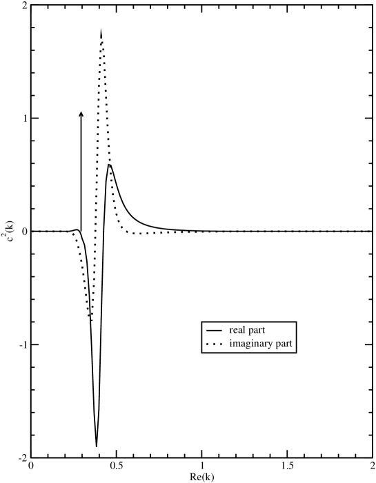
Figure 1: Distribution of the squared amplitudes $c^{2}(k)$ of the $2p_{3/2}$ proton state of a Woods-Saxon potential with a depth $V_{0}=65$ MeV, in the s.p. basis generated by a Woods-Saxon potential with a depth $V_{0}=70$ MeV. The Coulomb potential is assumed to be that of a uniformly charged sphere. The amplitudes of both real (solid line) and imaginary (dotted line) components of the wave function are plotted as a function of $\Re[k]$. The height of the arrow gives the squared amplitude of the $2p_{3/2}$ state contained in the basis.

The second example, shown in Fig. 2, deals with the case of a $2p_{3/2}$ state that is bound in both potentials. Here $V_{0}$=75 MeV and $V_{0}^{(B)}$=80 MeV, and the $2p_{3/2}$ state lies at $E$=–0.0923 MeV and $E$=–2.569 MeV, respectively. Here, the scattering component is almost negligible, which reflects the localized character of bound proton states. After the diagonalization, one obtains $E$=–2.568 MeV and $\Gamma$=1.73 keV for the $2p_{3/2}$ state, which is indeed very close to the exact result.

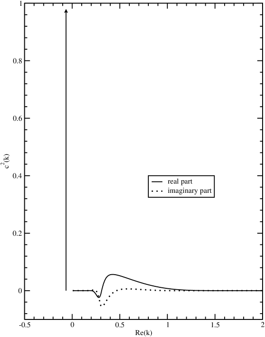
Figure 2: Similar as in Fig. 1 except for the bound $2p_{3/2}$ s.p. state of the WS potential with $V_{0}$=75 MeV expanded in the basis generated by another WS potential ($V_{0}^{(B)}$ = 80 MeV). The height of the arrow gives the squared amplitude of the bound $2p_{3/2}$ state at the value of –$\Im[k]$. (The corresponding $k-$value is purely imaginary.)

In the third example, the unbound $2p_{3/2}$ state ($E=$1.905 MeV and $\Gamma=$61.89 keV; $V_{0}$=70 MeV) is expanded in a WS basis containing the bound $2p_{3/2}$ level ($E$=–0.0923 MeV; $V_{0}^{(B)}$=75 MeV). As a consequence, the resonance’s width has to be brought by the scattering states. Nevertheless, the component of the $2p_{3/2}$ state of the basis is still close to one, whereas the continuum component plays a secondary role. Once again, one can see a Coulomb barrier effect: even if the expanded $2p_{3/2}$ state is unbound, its wave function is very localized due to the large Coulomb barrier; hence it has a large overlap with the bound $2p_{3/2}$ basis state. The diagonalization yields $E=$1.9065 MeV and $\Gamma=$58.9 keV, i.e., the discretization error is again close to 3 keV.

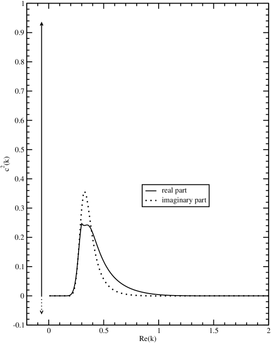
Figure 3: Similar as in Fig. 2 except for the $2p_{3/2}$ resonance of the WS potential with $V_{0}$=70 MeV expanded in the basis generated by another WS potential ($V_{0}^{(B)}$ = 75 MeV).

In the last example, shown in Fig. 4, the basis is that of the WS potential with a depth of 70 MeV, and the expanded state corresponds to a WS potential with $V_{0}$=75 MeV. This is the most interesting case since one expresses a bound (real) state in the basis which contains only complex wave functions. (The contribution from well bound $0p_{3/2}$ and $1p_{3/2}$ s.p. states is negligible.) As expected, the behavior of the amplitudes is very close to that of the previous example (see Fig. 3). Moreover, one can notice that the scattering states become important in the expansion when their energies approach the resonant state energy. The diagonalization gives $E=$–0.0925 MeV and $\Gamma=$-3.8 keV for the $2p_{3/2}$ state.

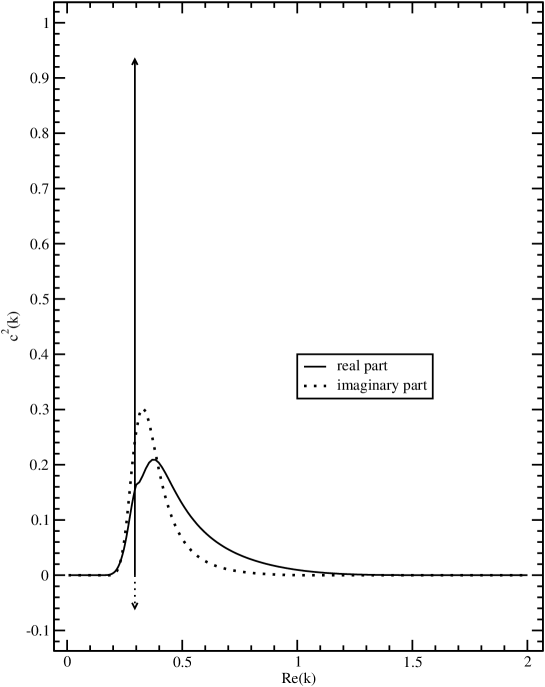
Figure 4: Similar as in Fig. 2 except for the $2p_{3/2}$ resonance of the WS potential with $V_{0}$=75 MeV expanded in the basis generated by another WS potential ($V_{0}^{(B)}$ = 70 MeV).

Summarizing this section, our numerical tests demonstrate that the one-body Berggren completeness relation works very well in the proton case involving the Coulomb potential. For other numerical tests, see Refs. Vertse et al. (1998) (study of the s.p. level density) and Lind et al. (1994) (study of the Berggren expansion in the pole approximation).

IV Spherical Gamow Hartree-Fock method

In our previous calculations of the He chain Michel et al. (2002, 2003), we used the s.p. basis of the WS potential representing ⁵He. This basis is appropriate at the beginning of the He chain, but when departing from the core nucleus, its quality deteriorates. For instance, the “⁵He” basis is not expected to be optimal when applied to the neutron-rich halo nucleus ⁸He because of the very different asymptotic behavior of this weakly bound system. The obvious remedy is to use the s.p. basis that is optimal for a given nucleus, that is the HF basis. However, since the Berggren ensemble used in GSM is required to possess spherical symmetry, HF calculations must be constrained to spherical shapes. Moreover, since in some cases one is interested in unbound nuclei lying beyond the drip line (particle resonances), the HF procedure has to be extended to unbound states. In the following, the HF-based procedure that meets the above criteria is referred to as the Gamow-Hartree-Fock (GHF) method.

Since, strictly speaking, the spherical HF potential cannot be defined for open shell nuclei, one has to resort to approximations. In this work, we tried two different ways of averaging the HF potential. The first ansatz is the usual uniform-filling approximation in which HF occupations are averaged over individual spherical shells. In the second ansatz, the deformed HF potential corresponding to non-zero angular momentum projection is averaged over all the magnetic quantum numbers. Both methods reduce to the true HF potential in the case of closed-shell nuclei.

IV.1 Average spherical HF potential

In the uniform-filling approximation no individual HF orbitals are blocked. The matrix elements of the HF potential $U_{\rm uf}$ between two spherical states $\alpha$ and $\beta$ carrying quantum numbers ($j,l$) are:

$$\langle\alpha|U_{\rm uf}|\beta\rangle = \langle\alpha|\hat{h}|\beta\rangle$$ (34)

$$+ \frac{1}{2j+1}\sum_{m,\lambda,m_{\lambda}}\frac{N(\lambda)}{2j_{\lambda}+1}\langle\alpha m\;\lambda m_{\lambda}|\hat{V}|\beta m\;\lambda m_{\lambda}\rangle$$

where $\hat{h}$ is the s.p. Hamiltonian (given by a WS+Coulomb potential), $\lambda$ is an occupied shell with angular quantum numbers ($j_{\lambda},l_{\lambda}$), $N(\lambda)$ is the number of nucleons occupying this shell, and $\hat{V}$ is the residual shell-model interaction.

To define the $M$-potential, one occupies (blocks) the s.p. states in the valence shell that have the largest angular momentum projections on the third axis. The resulting Slater determinant corresponds to the angular momentum $J$=$M$. For closed-shell nuclei ($M$=0) and for nuclei with one particle (or hole) outside a closed subshell ($M$=$j$), this Slater determinant can be associated with the ground state of the s.p. Hamiltonian. However, in other cases it corresponds to an excited state with $J$$>$0. Spherical $M$-potential, $U_{M}$, is defined by averaging the resulting HF potential over magnetic quantum number $m$:

$$\langle\alpha|U_{M}|\beta\rangle = \langle\alpha|\hat{h}|\beta\rangle$$ (35)

$$+ \frac{1}{N_{l,j}}\sum_{m=j+1-N_{l,j}}^{j}\sum_{\lambda}\langle\alpha m\;\lambda m_{\lambda}|\hat{V}|\beta m\;\lambda m_{\lambda}\rangle$$

where $N_{l,j}$ is the number of nucleons occupying the valence shell with quantum numbers $l,j$.

The $M$-potential is expected to work better for nuclei with one particle (or hole) outside the closed subshell. However, one can expect this potential to be not as good as $U_{\rm uf}$ when the Slater determinant with $J$=$M$ represents an excited state.

IV.2 Unbound HF states

While the HF procedure is well defined for the bound states, it has to be modified for the unbound s.p. states (resonant or scattering), even in the case of closed-shell nuclei. First, the effective nuclear two-body interaction has to be quickly vanishing beyond certain radius. Indeed, if it does not, the resulting HF potential diverges when $r\rightarrow+\infty$, thus providing incorrect s.p. asymptotics. Moreover, as resonant states are complex, the true self-consistent HF potential is complex. This is to be avoided, as the Berggren completeness relation assumes a real potential. However, since we are interested in the optimal basis-generating potential and not in the full-fledged complex-energy HF problem Kruppa et al. (1997), we simply take the real part of the (generally complex) HF potential.

IV.3 Treatment of the exchange part

As the residual interaction used in our shell-model calculations is finite range, its exchange part gives rise to a non-local potential. The HF equations solved in the coordinate space can be written as integro-differential equations. The standard method to treat such a HF problem is by means of the equivalent local potential Vautherin and Vénéroni (1957):

$$V_{\rm eq}(r)=v_{l}(r)+\frac{\int_{0}^{+\infty}v_{nl}(r,r^{\prime})u(r^{\prime})\;dr^{\prime}}{u(r)},$$ (36)

where we use the notation of Eq. (27). The resulting HF equations are local but potentials become state dependent. The main difficulty is the appearance of singularities in $V_{\rm eq}(r)$ due to the zeroes of the s.p. wave function. This problem is practically solved by replacing $u(r)$ with a small number (e.g., $10^{-3}$) in the denominator of Eq. (36) when $u(r)$ approaches zero, and by using splines to define the HF potential. The numerical accuracy is checked by calculating overlaps between different wave functions having the same ($j,l$) values. The overlaps are typically $10^{-5}$, which is small enough to consider wave functions orthogonal.

Let us note in passing that the demonstration of Sec. II.2 is valid when the non-local part of the potential is localized, as it is the case for the nuclear interaction. However, if one wants to explicitly consider the Coulomb HF potential between valence protons, one has to resort to approximations in order to avoid its infinite-range non-local part. One possibility is to use the so-called Slater approximation, which has been shown to work fairly well Skalski (2001). Another method, the so-called generalized local approximation, has been proposed in Ref. Bulgac, Lewenkopf and Mickrjukov (1995), where the Coulomb exchange term has been parametrized in terms of a coordinate-dependent effective mass. In any case, the effect of the approximate treatment of the Coulomb exchange term on the GHF basis is very small as compared to other uncertainties related to the construction of the GHF Hamiltonian.

IV.4 Choice of the average potential

In order to compare the quality of two GHF potentials, we inspect the binding energy (i.e., the expectation value of the GSM Hamiltonian) for several Li and He isotopes in the truncated GSM space. As discussed in Sec. V below, we took at most two particles in the GHF continuum. Due to this truncation, and as well as the discretization of the contour $L_{+}$ and the assumption of the momentum cut-off (the contour does not extend to infinity), the completeness relation of the resulting many-body shell-model basis is violated and, except for some special cases, the results obtained with different average potentials are different.

According to the variational principle, better basis-generating potentials must yield lower binding energies. Table 1 shows the binding energies of ^6,7,9He and ^7-11Li calculated in the GSM. Since ⁸He and ¹⁰He are closed-shell nuclei, both $U_{\rm uf}$ and $U_{M}$ are identical in these cases.

Table 1: Binding energies of the He and Li isotopes (in MeV) calculated in the GSM using the GHF basis with (i) the uniform-filling approximation potential $U_{\rm uf}$ or (ii) the $U_{M}$-potential. See Sec. IV.1 for definitions.

	6He	7He	9He	7Li	8Li	9Li	10Li	11Li
$U_{\rm uf}$	-1.038	-0.048	-2.357	-14.266	-15.521	-20.288	-18.082	-15.649
$U_{M}$	-0.984	-0.475	-2.418	-13.008	-15.094	-20.181	-17.749	-15.634

One can see that the uniform-filling approximation for the GHF potential works better for ⁷Li, ⁸Li, and ¹⁰Li, whereas the s.p. basis of the $M$-potential is a better choice for ⁷He. In all the remaining cases, the two potentials give results that are practically equivalent. In the particular case of ⁶He and ⁶Li (not displayed), there are at most two nucleons in the non-resonant continuum. Consequently, the shell-model spaces for ⁶He and ⁶Li are almost complete, and the results are almost independent on the choice of s.p. basis. Based on our tests, in our GHF calculations we use the uniform-filling approximation except for nuclei with one particle (hole) outside closed subshells where the $M$-potential provides a slightly more optimal s.p. basis.

V Gamow Shell Model description of the Lithium chain

V.1 Description of the calculation

In our previous studies Michel et al. (2002, 2003), we have used the s.p. basis generated by a WS potential which was adjusted to reproduce the s.p. energies in ⁵He. This potential (“⁵He” parameter set Michel et al. (2003)) is characterized by the radius $R$=2 fm, the diffuseness $d$=0.65 fm, the strength of the central field $V_{0}$=47 MeV, and the spin-orbit strength $V_{\rm so}$=7.5 MeV. As a residual interaction, we took the Surface Delta Interaction (SDI). However, when it comes to practical applications, SDI has several disadvantages. Firstly, it has zero range, so an energy cutoff has to be introduced; hence the residual interaction depends explicitly on the model space. Moreover, as the SDI interaction cannot practically be used to generate the HF potential (it produces a nonrealistic mean field), one is bound to use the same WS basis for all nuclei of interest, which is far from optimal as the number of valence particles increases. So, we have decided to introduce Michel et al. a finite-range residual interaction, the Surface Gaussian Interaction (SGI):

$$V^{\rm SGI}_{J,T}({\bm{r}}_{1},{\bm{r}}_{2})=V_{0}(J,T)\cdot\exp\left[-\left(\frac{{\bm{r}}_{1}-{\bm{r}}_{2}}{\mu}\right)^{2}\right]\cdot\delta{\left(|{\bm{r}}_{1}|+|{\bm{r}}_{2}|-2\cdot R_{0}\right)},$$ (37)

which is used together with the WS potential with the “⁵He” parameter set.

The Hamiltonian employed in our work can thus be written as follows:

$$\hat{H}=\hat{H}^{(1)}+\hat{H}^{(2)}$$ (38)

where $\hat{H}^{(1)}$ is the one-body Hamiltonian described above augmented by a hard sphere Coulomb potential of radius $R_{0}$ from the ⁴He core, and $\hat{H}^{(2)}$ is the two-body interaction among valence particles, which can be written as a sum of SGI and Coulomb terms. It is important to emphasize that the Coulomb interaction between valence protons can be treated as precisely at the shell-model level as the nuclear part. Indeed, the Coulomb two-body matrix elements in the HF basis can be calculated using the exterior complex scaling as decribed in Ref. Michel et al. (2003). Though not used in this paper, as we are considering only one valence proton in the shell model space, this feature of the Gamow Shell Model allows for a precise treatment of the Coulomb term.

The SGI interaction is a compromise between the SDI and the Gaussian interaction. The parameter $R_{0}$ in Eq. (37) is the radius of the WS potential, and $V_{0}(J,T)$ is the coupling constant which explicitly depends on the total angular momentum $J$ and the total isospin $T$ of the nucleonic pair. A principal advantage of the SGI is that it is finite-range, so no energy cutoff is, in principle, needed. Moreover, the surface delta term in (37) simplifies the calculation of two-body matrix elements, because they can be reduced to one-dimensional radial integrals. (In the case of other finite-range interactions, such as the Gogny force Dechargé and Gogny (1980), the radial integrals are two-dimensional.) Consequently, with SGI, an adjustment of the Hamiltonian parameters becomes feasible.

The Hamiltonian (38) is diagonalized in the Berggren basis generated by means of the GHF procedure of Sec. IV. This allows one to use the optimal spherical GHF potential for each nucleus studied; hence a more efficient truncation in the space of configurations with a different number of particles in the non-resonant continuum.

V.2 Choice of the valence space

The valence space for protons and neutrons consists of the $0p_{3/2}$ and $0p_{1/2}$ GHF resonant states, calculated for each nucleus, and the $\{ip_{3/2}\}$ and $\{ip_{1/2}\}$ $(i=1,\cdots,n)$, respectively complex and real continua generated by the same potential. These continua extend from $\Re[k]$=0 to $\Re[k]$=8 fm^-1, and they are discretized with 14 points (i.e., $n$=14). The $0p_{1/2}$ state is taken into account only if it is bound or very narrow. For the lightest isotopes considered, it is a very broad resonant state ($\Gamma\sim$ 5 MeV), and, on physics grounds, it is more justified to simply take a real $\{ip_{1/2}\}$ contour, so the completeness relation is still fulfilled.

Altogether, we have 15 $p_{3/2}$ and 14 or 15 $p_{1/2}$ GHF shells in the GSM calculation. The imaginary parts of $k$-values of the discretized continua are chosen to minimize the error made in calculating the imaginary parts of energies of the many-body states. Another continua, such as $s_{1/2}$, $d_{5/2}$, $\cdots$ are neglected, as they can be chosen to be real and would only induce a renormalization of the two-body interaction. We have checked Michel et al. (2002, 2003) that their influence on the binding energy of light helium isotopes is negligible. On the other hand, the $1s_{1/2}$ anti-bound neutron s.p. state is important in the heaviest Li isotopes (¹⁰Li, ¹¹Li) and plays a significant role in explaining the halo ground-state (g.s.) configuration of ¹¹Li Thompson and Zhukov (1994); Betan et al. (2004). At present, however, solving a GSM problem for ¹¹Li in the full $psd$ GHF space is not possible within a reasonable computing time.

Having defined a discretized GHF basis, we construct the many-body Slater determinants from all s.p. basis states (resonant and scattering), keeping only those with at most two particles in the non-resonant continuum. Indeed, according to our tests, as the two-body Hamiltonian is diagonalized in its optimal GHF basis, the weight of configurations involving more than two particles in the continuum is usually quite small, and they are neglected in the following. To illustrate this point, let us consider the $J^{\pi}$=$3/2^{-}$ ground state of ⁷Li. Since, in this case, there are only three valence particle, the complete calculation is possible. As seen in Table 2, the weight of the component with three particles in the non-resonant continuum, $L_{+}^{(3)}[\pi\nu^{2}]$ is indeed two orders of magnitude smaller than other configurations weights. The presence of $L_{+}^{(3)}[\pi\nu^{2}]$ modifies the weights of other configurations on a very ninor way. For the leading configuration, $0p_{3/2}[\pi]$$0p^{2}_{3/2}[\nu]$, without any particles in the non-resonant continuum, the effect is $\sim$8%. As a consequence, the neglect of the $L_{+}^{(3)}[\pi\nu^{2}]$ component leaves the overall structure of the state unchanged, and one can safely truncate the shell model space while slightly renormalizing the two-body residual interaction.

Table 2: Squared amplitudes of different configurations in the ground state of ⁷Li without truncation (second column) and with truncation to at most two particles in the non-resonant continuum (third column). The sum of squared amplitudes of all Slater determinants with $n$ particles (protons $[\pi]$ or/and neutrons $[\nu]$) in the non-resonant continuum is denoted by $L_{+}^{(n)}$.

Configuration	No Truncation	Truncation
$0p_{3/2}[\pi]$ $0p^{2}_{3/2}[\nu]$	0.561–i2.783$\cdot 10^{-4}$	0.612–i2.285$\cdot 10^{-4}$
$L_{+}^{(1)}[\pi]$	0.096+i4.732$\cdot 10^{-5}$	0.096+i4.980$\cdot 10^{-5}$
$L_{+}^{(1)}[\nu]$	0.184+i1.203$\cdot 10^{-4}$	0.164+i1.077$\cdot 10^{-4}$
$L_{+}^{(2)}[\nu^{2}]$	0.064+i2.419$\cdot 10^{-5}$	0.054+i1.600$\cdot 10^{-5}$
$L_{+}^{(2)}[\pi\nu]$	0.088+i7.032$\cdot 10^{-5}$	0.075+i5.508$\cdot 10^{-5}$
$L_{+}^{(3)}[\pi\nu^{2}]$	0.008+i1.621$\cdot 10^{-5}$	0

To calculate the first $2^{+}(T=0)$ of ⁶Li and in order to have the two first $5/2^{-}$ of ⁷Li, nevertheless, it is necessary to take into account the $0p_{1/2}$ states, even if they are broad. Indeed, without these states, the first $2^{+}(T=0)$ of ⁶Li does not exist at the level of pole approximation and as a consequence is impossible to find. Moreover, there is only one $5/2^{-}$ for ⁷Li at the level of pole approximation without the $0p_{1/2}$ states. As a consequence, one used the resonant $0p_{1/2}$ states in the basis to calculate these two states, thus deforming the $p_{1/2}$ contours in the complex plane so the resonant $0p_{1/2}$ states are enclosed. One also took twice as more points for these contours in order to further reduce discretization effects. To check that the two set of basis states are equivalent, one calculated the first $1^{+}$, $0^{+}$ and $2^{+}(T=1)$ with them. The first $3^{+}$ is not mentioned as no $p_{1/2}$ state, resonant or scattering, can enter its decomposition for obvious geometrical reasons. The comparison between the two is shown in Fig. 5, where it is clear that the two ways to calculate the eigenstates are equivalent.

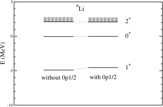
Figure 5: Eigenstates of ⁶Li calculated with and without the $0p_{1/2}$ resonant state in the basis.

V.3 The lithium chain

As a pilot example of GSM calculations in the space of proton and neutron states, we have chosen to investigate the Li chain. The continuum effects are very important in these nuclei, both in their ground states and in excited states. The nucleus ¹¹Li is also a well-known example of a two-neutron halo. In our $p$-space(s) calculation, we consider the one-body Coulomb potential of the ⁴He core, which is given by a uniformly charged sphere having the radius of the WS potential. It turns out that the inclusion of the one-body Coulomb potential modifies the GHF basis in lithium isotopes as compared to the helium isotopes, an effect which is usually neglected in the standard SM calculations.

Recent studies of the binding energy systematics in the $sd$-shell nuclei using the Shell Model Embedded in the Continuum (SMEC) Bennaceur et al. (1999, 2000) have reported a significant reduction of the neutron-proton $T$=0 interaction with respect to the neutron-neutron $T$=1 interaction in the nuclei close to the neutron drip line Luo et al. ; Michel et al. (2004). In SMEC, this reduction is associated with a decrease in the one-neutron emission threshold when approaching the neutron drip line, i.e., it is a genuine continuum coupling effect. The detailed studies in fluorine isotopes have shown that the reduction of the $T$=0 neutron-proton interaction cannot be corrected by any adjustment of the monopole components of the effective Hamiltonian. To account for this effect in the standard SM, one would need to introduce a particle-number-dependence of the $T$=0 monopole terms. Interestingly, it has recently been suggested Zuker (2003) that a linear reduction of $T$=0 two-body monopole terms is expected if one incorporates three-body interactions into the two-body framework of a standard SM.

Our GSM studies of lithium isotopes indicate that the reduction of $T$=0 neutron-proton interaction with increasing neutron number is essential. For example, if one uses the $V_{0}(J,T=0)$ strength adjusted to ⁶Li to calculate ⁷Li, the g.s. of ⁷Li becomes overbound by 13 MeV, and the situation becomes even worse for heavier Li isotopes. To reduce this disastrous tendency, in the first approximation, we have used a linear dependence of $T$=0 couplings on the number of valence neutrons $N_{n}$:

$$V_{0}(J=1,T=0)=\alpha_{10}\left[1-\beta_{10}(N_{n}-1)\right],$$ (39)

$$V_{0}(J=3,T=0)=\alpha_{30}\left[1-\beta_{30}(N_{n}-1)\right],$$ (40)

with $\alpha_{10}=-600$ MeV fm³, $\beta_{10}=-50$ MeV fm³, $\alpha_{30}=-625$ MeV fm³, and $\beta_{30}=-100$ MeV fm³. This linear dependence is probably oversimplified, as shown in Refs. Luo et al. ; Michel et al. (2004) where the proton-neutron $T$=0 interaction first decreases fast with increasing neutron number and then saturates for weakly bound systems near the neutron drip line. For the $T$=1 interaction, we have taken parameters $V_{0}(J=0,T=1)$ and $V_{0}(J=2,T=1)$ determined for the He ground states Michel et al. , as they provide reasonable results in the He chain.

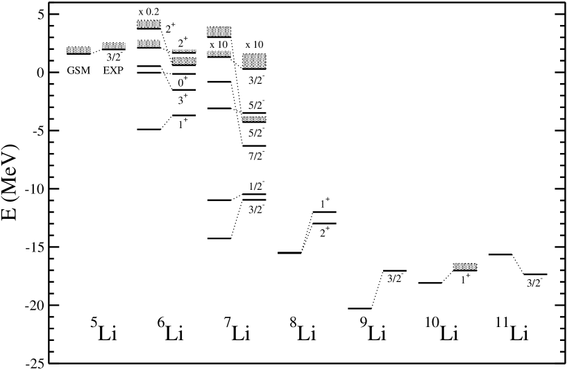
Figure 6: Experimental (EXP) and predicted (GSM) binding energies and spectra of lithium isotopes obtained with the SGI Hamiltonian. The resonance widths are indicated by shading. The energies are given with respect to the core of ⁴He. Experimental data are taken from Bohlen et al. (1997); (ensdf) (en(, ma().

The results of our GSM calculations for the neutron-rich Li isotopes are shown in Fig. 6. One obtains a reasonable description of the g.s. energies of lithium isotopes relative to the g.s. energy of ⁴He, but excited states are reproduced roughly. Clearly, the particle-number dependence of the matrix elements has to be further investigated in order to achieve the detailed description of the data. The absence of an anti-bound $s_{1/2}$ state in the Berggren basis is also likely responsible for large deviations with the data seen for ¹⁰Li and ¹¹Li.

In a number of cases, excited GSM states are calculated to lie above several decay thresholds, i.e., they are predicted to be unstable to, single-nucleon, deutron, proton+neutron emission, and/or $\alpha$ decay. The total decay width of a nucleus in a given GSM eigenstate is given by an imaginary part of its complex eigenenergy. Different open decay channels contribute incoherently to the total decay width and their respective partial width cannot be separated easily Okołowicz et al. (2003). In practical applications, however, one may calculate the spectroscopic factors for the separation of nucleon(s) or nucleon groups in a given GSM eigenstate, following the well-known procedures of the standard shell model Balashov et al. (1959); Wildermuth (1962), i.e., by calculating the probability to find a certain one- or many-particle configuration formed by $A-k$ and $k$ nucleons in a state of the $A$-nucleon system. We intend to implement this option in the future.

Table 3: Average isospin (41) calculated in GSM for various states in ^6,7Li.

$J^{\pi}$	1+	2${}_{1}^{+}$	2${}_{2}^{+}$	3/2- (g.s.)	1/2-	5/2-	7/2-	3/2-
$T_{av}$	0.01	0.023+i0.020	1+i0.015	0.509	0.514	0.507	0.505	1.503+i0.011

Due to the explicit presence of the Coulomb potential in the GSM, isospin is no longer conserved. In order to assess the isospin-mixing effect, for each shell model state $|\Psi\rangle$ we define the average isospin quantum number $T_{av}$ in the following way:

$$T_{av}=\frac{-1+\sqrt{1+4\langle\Psi|\hat{T}^{2}|\Psi\rangle}}{2}$$ (41)

where the isospin raising and lowering operators in $\hat{T}^{2}$ act on single-proton and single-neutron states with explicitly different asymptotic behavior. As seen in Table 3, the values of $T_{av}$ indicate very small isospin-mixing effects. The imaginary part for 2⁺ of ⁶Li and 3/2^- of ⁷Li comes from the fact these states are unbound. This result demonstrates that despite the presence of the Coulomb potential and despite a large coupling to the continuum in some cases, the isospin quantum number is still almost nearly conserved. That is, isospin is a very good characteristic of nuclear states, even if they are unbound, such as the second $3/2^{-}$ state of ⁷Li (which is a $T$=3/2 isobaric analogue of the ⁷He ground state) or the lowest $T$=1, $J^{\pi}$=2⁺ state of ⁶Li (which can be viewed as a $T$=1 isobaric analogue of the first excited state of ⁶He).

The identification of states can be problematic when the eigenstates have same angular momenta and parities. When their isospin is different, the calculation of the approximate isospin quantum number is useful to identify one state with its experimental counterpart, as was done with the two $2^{+}$ states of ⁶Li. For the two $5/2^{-}$ of ⁷Li, which have both $T=1/2$ experimentally, the consideration of their width can be used instead to identify them. Indeed, one of them is broad with a width of 880 keV, while the other is narrower with a width of 89 keV. As one $5/2^{-}$ state has to occupy $0p_{1/2}$ broad resonant states at the level of pole approximation while the other does not, the latter state can be associated with the $5/2^{-}$ with a width of 89 keV, while the former can be associated with the $5/2^{-}$ with a width of 880 keV.

VI Conclusions

The Gamow Shell Model, which has been introduced only very recently Michel et al. (2002, 2003), has proven to be a reliable tool for the microscopic description of weakly bound and unbound nuclear states. In the He isotopes, GSM, with either SDI or SGI interactions, was able to describe fairly well binding energy patterns and low-energy spectroscopy, in particular the Borromean features in the chain ^4-8He Michel et al. (2003, ). Using the finite-range SGI interaction made it possible to perform calculations in the GHF basis, thus designing the optimal Berggren basis for each nucleus.

In the Li isotopes, the results crucially depend on the $T$=0 interaction channel. It was found that the $T$=0 force should contain a pronounced density (particle-number) dependence which originates from the coupling to the continuum and leads to an effective renormalization of the neutron-proton coupling. This effect cannot be absorbed by the modification of $T$=0 monopole terms in the standard SM framework. The effective renormalization of ($J=1,T=0$) and ($J=3,T=0$) couplings, and, to a lesser extent, other coupling constants found in the present GSM studies has to be further investigated. To better take into account all these effects, calculations with a finite-range, density-dependent interaction inspired by the Gogny force Dechargé and Gogny (1980) are now in progress. The three main problems related to the realistic GSM calculations are the treatment of the center of mass (essential, especially in the context of halo nuclei), the inclusion of anti-bound states Thompson and Zhukov (1994); Betan et al. (2004); Vertse et al. (1989); Hagen et al. , and the handling of very large shell-model spaces.

For that matter, the successful application of GSM to heavier nuclei is ultimately related to the progress in optimization of the GSM basis, related to the inclusion of the non-resonant continuum configurations. A promising development is the adaptation of the density matrix renormalization group method White (1993) to the genuinely non-hermitian SM problem in the complex-$k$ plane using the $j$-scheme Rotureau et al. (2004); Michel et al. .

In summary, in this paper we report the proof-of-principle proton-neutron calculations using the Gamow Shell Model. Our single-particle proton Hamiltonian contains the Coulomb term that explicitly breaks isospin symmetry. In order to extend GSM calculations to open-proton systems, the Berggren completeness relation has been extended to the case of the Coulomb potential. The completeness relation has also been derived for nonlocal interactions that naturally appear in the GHF method, a Hartree-Fock inspired procedure to optimize the s.p. basis. According to GSM, the isospin mixing-effects are very weak, even for high-lying unbound states of Li isotopes.