Short-range nucleon-nucleon correlation effects in
photon- and electron-nucleus reactions

Abstract

The role played by nucleon-nucleon short-range correlations in photon- and electron-nucleus reactions is analyzed with a model which includes all the diagrams containing a single correlation function. The excitation of low-lying high-spin states, the reactions (e,e’), (e,e’N) and ($\gamma$,N) and the two-proton emission by both electrons and real photons are investigated. The results obtained for doubly-closed shell nuclei show that ($\gamma$,pp) appears to be the most adequate process to identify short-range correlations in the clearer way.

I The model

In these last years we have developed a model to describe electromagnetic responses of nuclei with $A>4$ by considering also SRC. Our model has been applied to describe inclusive (e,e’) processes co98 ; mok00 ; co01 as well as one- mok01 ; ang02 and two-nucleon ang03 ; ang04 emission processes induced by both electrons and real photons, providing a unified and consistent description of all these processes.

The linear response of the nucleus to an external operator $O({\bf q})$ can be written as

$$S({\bf q},\omega)\,=\,-\frac{1}{\pi}\,\rm{Im}\,\left[\sum_{n}\,\xi_{n}^{+}({\bf q})\,(E_{n}-E_{0}-\omega+i\eta)^{-1}\,\xi_{n}({\bf q})\right]\,,$$ (1)

where we have defined

$$\xi_{n}({\bf q})\,=\,\frac{\langle\Psi_{n}|\,O({\bf q})\,|\Psi_{0}\rangle}{\langle\Psi_{n}|\Psi_{n}\rangle^{\frac{1}{2}}\,\langle\Psi_{0}|\Psi_{0}\rangle^{\frac{1}{2}}}$$ (2)

This function involves the transition matrix element between the initial and the final states of the nucleus. These states are constructed by acting with a correlation operator $F$ on uncorrelated Slater determinants, as established by the Correlated Basis Function theory: $|\Psi_{0}\rangle\,=\,F\,|\Phi_{0}\rangle$ and $|\Psi_{n}\rangle\,=\,F\,|\Phi_{n}\rangle$.

In our model we have considered only scalar correlation functions of the type

$$F\,=\,\displaystyle\prod_{i<j}\,f_{ij}\,,$$ (3)

which commute with the transition operator $O({\bf q})$. Thus the $\xi$ function can be written as

$$\xi_{n}({\bf q})\,=\,\frac{\langle\Phi_{n}|\,O({\bf q})\,\displaystyle\prod_{i<j}\,(1+h_{ij})\,|\Phi_{0}\rangle}{\langle\Phi_{0}|\displaystyle\prod_{i<j}\,(1+h_{ij})\,|\Phi_{0}\rangle}\,\left[\frac{\langle\Phi_{0}|\displaystyle\prod_{i<j}\,(1+h_{ij})\,|\Phi_{0}\rangle}{\langle\Phi_{n}|\displaystyle\prod_{i<j}\,(1+h_{ij})\,|\Phi_{n}\rangle}\right]^{\frac{1}{2}}\,,$$ (4)

where $h_{ij}=f^{2}_{ij}-1$. We assume that the operator $O({\bf q})$ which induces the transitions is a one-body operator. We perform the full cluster expansion of this expression and the presence of the denominator allows us to eliminate the unlinked diagrams. At this point we insert the main approximation of our model by truncating the resulting expansion such as only those diagrams which involve a single correlation function $h$ are retained

$$\xi_{n}({\bf q})\rightarrow\xi^{1}_{n}({\bf q})\,=\,\langle\Phi_{n}|\,O({\bf q})\,(1+\sum_{i<j}\,h_{ij})\,|\Phi_{0}\rangle_{L}\,.$$ (5)

In the above expression the subscript $L$ indicates that only linked diagrams are included in the expansion.

Figure 1: Meyer-like diagrams contributing to $\xi^{1}_{\rm 1p1h}({\bf q})$.

Figure 2: Meyer-like diagrams contributing to $\xi^{1}_{\rm 2p2h}({\bf q})$.

For one-particle one-hole final states, the function $\xi$ includes three terms:

$$\xi^{1}_{\rm 1p1h}({\bf q})\,=\,\langle\Phi_{\rm 1p1h}|\,O({\bf q})\,|\Phi_{0}\rangle+\,\langle\Phi_{\rm 1p1h}|\,O({\bf q})\,\displaystyle\sum^{A}_{j>1}\,h_{1j}\,|\Phi_{0}\rangle+\,\langle\Phi_{\rm 1p1h}|\,O({\bf q})\,\displaystyle\sum^{A}_{1<i<j}\,h_{ij}\,|\Phi_{0}\rangle\,.$$ (6)

The contributions of the various terms of the above expression are shown in Fig. 1 in terms of Meyer-like diagrams. In addition to the uncorrelated transition represented by the one-point diagram (1.1), also four two-point (2p) diagrams and six three-point (3p) diagrams are present. All these terms are necessary to get a proper normalization of the nuclear wave functions. In the figure, the black squares represent the points where the external operator is acting, the dashed lines represent the correlation function $h$ and the continuous oriented lines represent the single-particle wave functions. The letters $h$, $i$ and $k$ label holes, while $p$ labels a particle. A sum over $i$ and $k$ is understood.

In the case one has two-particle two-hole final states, the function $\xi$ includes two terms:

$$\xi^{1}_{\rm 2p2h}({\bf q})\,=\,\langle\Phi_{\rm 2p2h}|\,O({\bf q})\,\displaystyle\sum^{A}_{1<j}\,h_{1j}\,|\Phi_{0}\rangle\,+\,\langle\Phi_{\rm 2p2h}|O(\,{\bf q})\,\displaystyle\sum^{A}_{1<i<j}\,h_{ij}\,|\Phi_{0}\rangle\,.$$ (7)

The first term consists of four 2p diagrams. The second one results from the sum of eight 3p diagrams. As in the previous case, this set of diagrams conserves the correct normalization of the nuclear wave functions.

Our model has been tested by comparing our results for the nuclear matter charge response functions with those obtained by considering the full cluster expansion. In these calculations the correlation used has been the scalar part of a complicated state dependent correlation fixed to minimize the binding energy in a Fermi Hypernetted chain calculation with the Urbana V14 NN potential wirin . We have found ama98 an excellent agreement between the results of the two calculations, and this gave us confidence to extend the model to other situations.

Figure 3: Nuclear matter longitudinal responses for $q=300$, 400 and 550 MeV/$c$ and $k_{F}=1.09$ fm^-1. Dashed lines represent the Fermi gas responses, the dashed-dotted lines have been obtained adding the two-point diagrams, while the full lines show the results of the complete calculations where all diagrams of Fig. 1 have been included. The nucleon form factors have been taken from Ref. hoel .

Figure 4: Correlation functions used in our calculations.

In Fig. 3 we show the effect of the different diagrams shown in Fig. 1. The dashed curves represent the uncorrelated Fermi gas result. The dashed-dotted curves show the effect of adding the 2p diagrams and, finally, the full curves give the final result after including the 3p diagrams. One can appreciate how 2p and 3p diagram contributions interfere destructively. This is a general characteristic of all our results.

In order to determine the sensitivity of our results to the details of the SRC we have considered three different correlation functions which are shown in Fig. 4. Two corrrelations, labeled $G$ and $S3$, are fixed by minimizing the energy functional calculated with a nuclear hamiltonian containing the Afnan and Tang NN potential ari96 . The first correlation is of gaussian type, $f(r)=1-a\exp\left(-br^{2}\right)$, and the minimization is done with respect to $a$ and $b$, obtaining $a$=0.7 and $b$=2.2 fm^-2. The $S3$ correlation is determined by using the Euler procedure, in which the minimization is carried out with respect to a single parameter, the healing distance. The $V8$ correlation is the scalar part of a state dependent correlation function fixed again with the Euler procedure but for a hamiltonian which includes the NN Argonne $V8^{\prime}$ plus the Urbana IX three body potentials fab00 .

Despite the small differences observed between the three correlation functions, we shall show that, in various cases, they can produce rather different results.

II Results

II.1 Inclusive (e,e’) processes

We start our study with the inclusive (e,e’) processes. Here we have investigated both the excitation of low-lying high-spin states and the quasi-elastic peak. In these calculations we have considered only the one-body charge and current operators.

The excitation of low-lying nuclear excited states was investigated to test the claim of Pandharipande, Papanicolas and Wambach pandha84 . These authors ascribed to SRC the quenching shown by the experimental data with respect to the calculations. It was argued that SRC produce the partial occupation of the single particle states around the Fermi level and this gives rise to the reduction in the cross sections.

	Jπ	$E$ (MeV)	p-h pairs	IPM		Correlated
				$Q$	$\chi^{2}$	$Q$	$\chi^{2}$
16O	4-	18.98	$\pi$ 1d5/2 1p${}_{3/2}^{-1}$
				0.67	26.35	0.66	35.06
			$\nu$ 1d5/2 1p${}_{3/2}^{-1}$
208Pb	9+	5.01	$\nu$ 2g9/2 1i${}_{13/2}^{-1}$	0.38	5.92	0.37	7.17
	9+	5.26	$\pi$ 1h9/2 1h${}_{11/2}^{-1}$	0.59	2.09	0.59	2.10
	10-	6.283	$\nu$ 1j15/2 1i${}_{13/2}^{-1}$	0.34	9.12	0.34	9.29
	10-	6.884	$\pi$ 1i13/2 1h${}_{11/2}^{-1}$	0.33	6.05	0.33	6.05
	12-	6.437	$\nu$ 1j15/2 1i${}_{13/2}^{-1}$	0.70	3.35	0.68	3.57
	12-	7.064	$\pi$ 1i13/2 1h${}_{11/2}^{-1}$	0.28	7.64	0.27	8.85
	14-	6.745	$\nu$ 1j15/2 1i${}_{13/2}^{-1}$	0.39	5.53	0.39	5.53
$\theta=90^{0}$	10+	5.920	$\nu$ 1i11/2 1i${}_{13/2}^{-1}$	0.63	18.90	0.69	20.63
$\theta=160^{0}$	10+	5.920	$\nu$ 1i11/2 1i${}_{13/2}^{-1}$	0.88	28.91	0.95	32.15
$\theta=90^{0}$	12+	6.100	$\nu$ 1i11/2 1i${}_{13/2}^{-1}$	0.52	7.55	0.57	8.76
$\theta=160^{0}$	12+	6.100	$\nu$ 1i11/2 1i${}_{13/2}^{-1}$	0.39	12.70	0.42	14.84

Table 1: Quenching factors obtained for the different excited states. The excitation energies $E$, the particle-hole pairs considered and the quenching factors $Q$ and the $\chi^{2}$ obtained for the calculations without and with SRC are given. In the case of the electric states the quenching factors have been obtained for the full cross section and the corresponding scattering angles have been indicated.

The effect of SRC as calculated in our model is very small. In order to quantify it, we have determined the quenching factor for different excited states. It is defined as the multiplying factor needed to bring the theoretical results in agreement with the experimental data. The values obtained by minimizing the corresponding $\chi^{2}$ are shown in Table 1. As we can see, the values obtained with and without SRC are very similar. Only in the cases analyzed for electric states (last four rows), the quenching factors increase by more than 5% after SRC are included. However, the values obtained are still far from 1. In these calculations the $S3$ correlation function has been used.

It is interesting to note the cases of the high-spin magnetic states in ²⁰⁸Pb, $12^{-}$ and $14^{-}$, which were those quoted by Pandharipande et al. in pandha84 . We see here that they are almost insensitive to the SRC.

Now we analyze the (e,e’) process in the quasi-elastic peak. The calculations we have performed for ¹⁶O and ⁴⁰Ca co01 have shown that the SRC produce very small effects in both the longitudinal and the transverse responses. The maximum variation in the peaks is around 2%, certainly within the range of the uncertainties of the calculations (for example, those due to the nucleon form factor choice).

In Fig. 5 we show the differences between correlated and uncorrelated responses after including the 2p (solid curves) and also the 3p (dashed curves) diagrams, for both the $S3$ and $V8$ correlations. The left (right) panels of the figure show the longitudinal (transverse) responses. Three values of the momentum transfer have been considered. As we can see, the inclusion of the 3p diagrams always reduces the effects produced by the 2p diagrams alone.

Figure 5: Differences between correlated and uncorrelated responses for ¹⁶O(e,e’), after including the 2p (solid curves) and also the 3p (dashed curves) diagrams, for both the $S3$ and $V8$ correlations, for the longitudinal and the transverse responses and for 300, 400 and 500 MeV/$c$.

In addition, it is interesting to point out the different behavior shown by the two correlation functions used here. The 2p contributions are positive for $S3$ and negative for $V8$ and the total contribution in case of the $S3$ function is always larger than that of the $V8$.

Despite this, it is worth to notice that SRC reduce the longitudinal response and increase transverse one. This is due to the fact that the diagram 2.3 of the 1p1h term (see Fig. 1) does not contribute to the transverse response.

II.2 One-nucleon emission

Now we discuss the main results we have obtained for one-nucleon emission processes mok01 ; ang02 . In these calculations, in addition to the usual one-body charge and current operators, one has to consider also the Meson Exchange Currents (MEC). Our analysis of the role of these currents ang02 shows that their contributions become small for momentum transfer values larger than 300 MeV/c. For this reason we neglect them in (e,e’p) processes. On the contrary, MEC are relevant in photo-emission processes. Specifically, in this case, we have considered the so-called seagull, pion-in-flight and $\Delta$-isobar currents.

In the nucleon emission knock-out processes, the wave functions of the hole states have been described by using a real Woods-Saxon potential, and those of the emitted particles by an optical potential Schw .

Figure 6: Panels (a)-(d) show the cross sections of the ¹⁶O(e,e’p) process as a function of the nucleon initial momentum $p_{i}=|{\bf p}-{\bf q}|$. The proton is emitted from the $1p_{1/2}$ level. The cross sections have been calculated for $\omega=128$ MeV and $|{\rm p}|=444$ MeV/$c$. Left (right) panels correspond to perpendicular (parallel) kinematics. The dashed curves include the uncorrelated and the 2p diagrams. The full curves include also the 3p diagrams. The panels (e)-(h) show the differences between the correlated and uncorrelated cross sections, divided by the maximum values of the uncorrelated cross sections, $\sigma_{\rm max}$. Results for both the $S3$ and $V8$ correlations are shown.

Panels (a)-(d) of Fig. 6 show the cross section for the ¹⁶O(e,e’p) process when the proton is emitted from the 1p_1/2 hole, for perpendicular (left panels) and parallel (right panels) kinematics. Calculations have been done for fixed values of $\omega=128$ MeV and $|{\rm p}|=444$ MeV/$c$. The dashed curves show the results obtained by including the 2p diagrams, while the full curves are obtained if 3p diagrams are added. In the scale of the figures, these last curves overlap almost exactly with those obtained without SRC (which are not shown in the figure). The effects of the SRC are always very small. In order to emphasize these effects, we show in the panels (e)-(h) of Fig. 6 the differences between correlated and uncorrelated cross sections, of the above calculations. We see again that the cross sections obtained for the $S3$ and $V8$ correlations show a very different behavior if only the 2p contributions are included, while the addition of the 3p diagrams produces rather similar results in both cases. This basic results does not change too much in other kinematic conditions, for example if the proton is emitted from the 1p_3/2 or 1s_1/2 hole state, or if different values of the momentum transfer are considered ang02 .

Figure 7: Relative differences between correlated and uncorrelated cross sections, for the ¹⁶O($\gamma$,p) process, for the three correlation functions considered and for two values of the energy transfer $\omega$. The proton is emitted from the $1p_{1/2}$ level.

Figure 8: Angular distributions for the ¹⁶O($\gamma$,p) process, calculated without SRC (thin full curves) and with the $S3$ (thick full curves), $V8$ (dashed curves) and $G$ (dotted curves) correlations. The proton is emitted from the $1p_{1/2}$ level.

Figure 9: Angular distributions of the ¹⁶O($\gamma$,p) process, calculated without SRC and MEC (thin full curves), by adding only the $S3$ correlation (dotted curves), by adding only the MEC (dashed curves) and with all the contributions (thick full curves), one-body plus SRC plus MEC. The proton is emitted from the $1p_{1/2}$ level.

Now we analyze the photoemission process. Fig. 7 shows, for the ¹⁶O($\gamma$,p) process, the relative differences between correlated and uncorrelated responses when only the 2p diagrams are included (dashed curves), and when also the 3p diagrams are considered (solid curves). Again, one can see how the contributions of the 3p diagrams cancel those due to the 2p ones in all cases. However, the full effect of the SRC for the $S3$ correlation (upper panels) shows a different sign with respect to that obtained with the $V8$ (middle panels) and with the $G$ (lower panels) correlations. Furthermore we point out that the order of magnitude of the correlation effects obtained with the $G$ correlation are about a factor $4$ larger than those obtained with the other correlation functions.

Fig. 8 shows the angular distribution for the ¹⁶O($\gamma$,p) calculated for various incident photon energies. In this figure, the uncorrelated cross sections, which are shown by the thin full curves, are compared with those obtained by using the $S3$ (thick full curves), $V8$ (dashed curves) and $G$ (dotted curves) correlation functions. A comparison between the SRC effects presented in this figure and those presented in Fig. 6 shows that the ($\gamma$,p) process has a larger sensitivity to the SRC functions that the (e,e’N).

As we have already mentioned, MEC effects are not negligible in photoemission reactions. In Fig. 9 we show the same cross sections of Fig. 8, but now with the MEC included. In Fig.9 the thin full lines represent the results obtained using the one-body currents only, i.e. without considering SRC and MEC. The addition of SRC (dotted curves) produces a modification much smaller than that found if only MEC are included (dashed curves). Thick solid curves correspond to the full results and it is evident that MEC dominate even in the large angle region, where SRC effects show up in a clearer way.

II.3 Two-proton emission

We finally discuss the two-proton emission processes induced by electrons ang03 and photons ang04 . In these processes the bare one-body currents contribution is absent. The one-body currents act only if linked to the SRC. When two-like particles are emitted, in our case two protons, the MEC produced by the exchange of charged mesons are not active. This means that in the two-proton emission, the only MEC competing with the SRC are $\Delta$ current due to the exchange of a chargeless pion. The description of the single particle wave functions is the same as that adopted for the single nucleon knock out. We have studied two-proton knock out from ¹²C, ¹⁶O and ⁴⁰Ca. The final states of the residual nuclei considered in our calculations are given in Table 2.

	12C	16O	40Ca
$0_{1}^{+}$	(1p3/2)-2	(1p1/2)-2	(1d3/2)-2
$0_{2}^{+}$		(1p3/2)-2	(2s1/2)-2
$1^{+}$		(1p1/2)-1 (1p3/2)-1	(1d3/2)-1 (2s1/2)-1
$2_{1}^{+}$	(1p3/2)-2	(1p1/2)-1 (1p3/2)-1	(1d3/2)-2
$2_{2}^{+}$		(1p3/2)-2	(1d3/2)-1 (2s1/2)-1

Table 2: Two-hole compositions of the nuclear final states of the residual nuclei for the two proton emission process we have considered.

Figure 10: Angular distributions of the (e,e’pp) cross sections for ¹⁶O, for different final states (see Table 2) and for the three correlation functions.

Figure 11: (e,e’pp) cross sections for ¹⁶O (left panels) and ⁴⁰Ca (right panels). The dotted curves have been obtained with 2p diagrams only. The dashed lines show the results obtained by adding 3p diagrams, and the solid lines those obtained by including also the $\Delta$ currents. The gaussian correlation has been used.

In Fig. 10 we show the (e,e’pp) cross sections for ¹⁶O, calculated for different final states with the three correlation functions shown in Fig. 4. In Fig. 10 the cross sections are shown as a function of the emission angle of one of the emitted protons. We have assumed coplanar kinematics, and we fixed the energy and emission angle of the other proton at 40 MeV and $60^{o}$ respectively. The incident electron energy has been chosen to be 800 MeV and the energy and momentum transferred to the nucleus have been fixed at 100 MeV and 400 MeV/$c$, respectively. The results of Fig. 10 show that the SRC modify the size of the cross sections, while the shape is maintained. The cross section obtained for the $S3$ and $V8$ are a factor 2 smaller than those found for the $G$ correlation. The $1^{+}$ is out of the systematic because it is dominated by the $\Delta$ current. Similar results are obtained for ¹²C and ⁴⁰Ca ang03 .

The fact that the $\Delta$ current dominates the $1^{+}$ cross sections is evident also from the results shown in Fig. 11, where the cross sections obtained with the gaussian correlation for ¹⁶O and ⁴⁰Ca are presented for three different final states. These calculations have been done for the same kinematics of Fig. 10. In Fig. 11, the dotted lines show the results obtained with the 2p diagrams only, while the dashed and solid lines have been obtained by adding first the 3p diagrams and then the $\Delta$ currents. The 3p diagrams reduce the cross sections obtained with the 2p diagrams only. This reduction depends from the angle of the emitted proton. This is particularly clear in the case of the $2^{+}$ states.

The last process we discuss is ($\gamma$,pp). In Fig. 12 we show the angular distributions of the cross sections corresponding to the three nuclei we are investigating. We have considered the case when the remaining nucleus is left in its ground state. The results have been obtained by using the three correlation functions of Fig. 4. Again, the main differences are in the size of the cross sections.

	12C		16O		40Ca
	$S3$	$V8$	$S3$	$V8$	$S3$	$V8$
$0_{1}^{+}$	0.73 $\pm$ 0.11	0.52 $\pm$ 0.05	0.10 $\pm$ 0.11	0.20 $\pm$ 0.05	0.15 $\pm$ 0.03	0.22 $\pm$ 0.04
$0_{2}^{+}$			0.83 $\pm$ 0.16	0.60 $\pm$ 0.08	0.37 $\pm$ 0.07	0.44 $\pm$ 0.07
$1^{+}$			0.97 $\pm$ 0.08	0.76 $\pm$ 0.07	0.37 $\pm$ 0.04	0.36 $\pm$ 0.06
$2_{1}^{+}$	0.56 $\pm$ 0.13	0.52 $\pm$ 0.08	0.25 $\pm$ 0.05	0.30 $\pm$ 0.04	0.22 $\pm$ 0.05	0.24 $\pm$ 0.03
$2_{2}^{+}$			0.54 $\pm$ 0.13	0.52 $\pm$ 0.08	0.54 $\pm$ 0.07	0.48 $\pm$ 0.05

Table 3: Ratio of the $S$ factor (see Eq. 8) calculated for the $S3$ and $V8$ correlations and that for the $G$ correlation, averaged on the $\theta_{2}$ variable.

In order to have a concise information, the integrated quantities

$$S^{\rm(SRC)}\,=\,\displaystyle\int{\rm d}\theta_{1}\sin\theta_{1}\frac{{\rm d}^{5}\sigma^{\rm(SRC)}(\theta_{1})}{{\rm d}\Omega_{1}{\rm d}\epsilon_{2}{\rm d}\Omega_{2}}$$ (8)

have been calculated for the various final states and for various emission angles of the second proton. The mean values of the ratios between the $S$ factors calculated with the $S3$ and $V8$ correlations and those calculated with the $G$ correlations are given in Table 3. All the values in the table are smaller than 1 and this means that $G$ correlation produce the largest cross sections.

Figure 12: Angular distributions of the ($\gamma$,pp) cross sections for the three different nuclei considered. The kinematics variables have been fixed as $\omega=100$ MeV, $\theta_{2}=90^{o}$ and $\epsilon_{2}$=40 MeV. The final states are the ground states of the $A-2$ nuclei, this corresponds to the $0^{+}_{1}$ states of Table 2. The full lines have been obtained with the gaussian correlation, the dotted ones with the S3 correlation and the dashed lines with the V8 correlation.

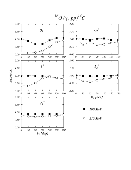
Figure 13: Ratio $S(C)/S(C\Delta)$ (see Eq. (8)), calculated for various values of $\theta_{2}$ and for photon energies of 100 and 215 MeV. The calculations have been done with $\epsilon_{2}$=40 MeV. The dashed lines have been drawn to guide the eyes.

Figure 14: Cross sections for ¹⁶O ($\gamma$,pp) ¹⁴C in superparallel back to back kinematics with $\theta_{2}=180^{o}$. The full lines have been obtained by considering both SRC and $\Delta$ terms, while the dashed lines show the results obtained without the $\Delta$ terms.

Figure 15: Angular distributions for ¹⁶O ($\gamma$,pp) ¹⁴C, for the $0^{+}_{1}$ final state, in symmetric kinematics. The full lines show the results obtained by considering both SRC and $\Delta$-currents. The results shown by the dashed lines have been obtained with SRC only. The numbers characterizing the two panels indicate, in MeV, the photon energy.

Figure 16: Same as in Fig. 14 for the three correlation functions used.

Figure 17: Angular distributions of the ¹⁶O ($\gamma$,pp) ¹⁴C cross sections for the $0^{+}_{2}$ final state. The numbers in the various panels indicate, in MeV, the values of $\epsilon_{2}$. The meaning of the lines is analogous to that of Fig. 16.

The second aspect of interest concerns the role of the $\Delta$ current. Fig. 13 shows the ratio between the $S$ factor calculated with SRC only with that obtained by adding the $\Delta$ currents contribution as a function of the angle $\theta_{2}$ of the second emitted proton. The reaction considered is ¹⁶O($\gamma$,pp) and the various panels show the results obtained for the different final states of the ¹⁴C. Two different photon energies have been used.

The effects of the $\Delta$ are smaller at 100 MeV than at 215 MeV, but they show a strong dependence on the final state of the residual nucleus and on the proton emission angle. For $\omega=100$ MeV, all the ratios, except for some cases, are very close to unity, showing a small effect of the $\Delta$ currents, even in the case of the $1^{+}$ state. In general, the (e,e’pp) reaction showed larger sensitivity to the $\Delta$ currents.

We found analogous results in other kinematics. Fig. 14 shows the effect of the $\Delta$ in the superparallel back-to-back kinematics. Again the $\Delta$ appears to have scarce relevance at $\omega=100$ MeV. Nevertheless there is noticeable effect for the $0^{+}_{1}$ state at high values of the recoil momentum.

However, it is possible to find kinematics where the $\Delta$ is important even at 100 MeV. This is what Fig. 15 shows. In this figure the results obtained for the $0^{+}_{1}$ state in the ¹⁶O($\gamma$,pp)¹⁴C reaction in symmetric kinematics are presented.

In all the results presented so far, those obtained with the gaussian correlation show the largest SRC effects, as Figs. 10 and 12 indicate. This trend regards the full angular distribution of one of the emitted protons after fixing the rest of the kinematics. By selecting specific kinematics, in other words, by choosing some peculiar angular distribution set ups, it is possible to find situations where this general feature is not present. An example of this is given in Fig. 16, where the cross sections calculated for the three different correlation functions in superparallel back-to-back kinematics are shown. It is evident how the case of the $0^{+}_{2}$ is out of the general trend observed for the other states.

To understand the results of Fig. 16, we show in Fig. 17 the full angular distributions of the emitted proton for various energies of the other proton. The cross sections of the $0^{+}_{2}$ panel in Fig. 16, have been obtained by selecting the values at $\theta_{1}=0^{o}$ in Fig. 17, and other more. The cross sections obtained with the gaussian correlation gives the largest integral in all the panels of Fig. 17, as expected. By selecting the $\theta_{1}=0^{o}$ values, one finds the anomaly of a deep minimum of the full lines, and this produces the anomalous behaviour shown in Fig. 16.

III Conclusions

The effects of the SRC in inclusive and one-nucleon emission processes are rather small, within the uncertainties of the calculations due to the arbitrary choice of the input parameters.

In these processes, the uncorrelated one-body responses dominate. There are situations in ($\gamma$,N) reactions showing certain sensitivity to the SRC. Unfortunately these are also the situations where the contribution of MEC is large, even larger than that of the SRC.

The emission of two nucleons has various advantages, the main one is that the one-body uncorrelated terms are absent. However there is competition between MEC and SRC. The MEC effects can be reduced by selecting the emission of two-like nucleons. In this case the only contribution of the MEC is due to the $\Delta$ currents with the exchange of a chargeless pion.

A priori the longitudinal response of the (e,e’pp) process can provide a very clean signature of the SRC since the $\Delta$ currents do not contribute. However, the extraction of this response requires a super Rosenbluth separation, which is, from the experimental point of view, a rather difficult procedure. The alternative is to look for situations where the $\Delta$ currents produce small effects.

The ($\gamma$,pp) process has a number of advantages with respect to (e,e’pp). First, only the transverse response is present. Second, the $\Delta$ current effects are minimal at the photon point and, as we have shown, these effects can be made almost negligible by an adequate choice of the kinematics.

References

- (1) G. Co’, A.M. Lallena, Phys. Rev. C 57 (1998) 145
- (2) S.R. Mokhtar, G. Co’ and A.M. Lallena, Phys. Rev. C 62 (2000) 067304.
- (3) G. Co’ and A. M. Lallena, Ann. Phys. (N.Y.) 287 (2001) 101.
- (4) S. R. Mokhtar, M. Anguiano, G. Co’ and A. M. Lallena, Ann. Phys. (N.Y.) 292 (2001) 67.
- (5) M. Anguiano, G. Co’, A. M. Lallena and S.R. Mokhtar, Ann. Phys. (N.Y.) 296 (2002) 235.
- (6) M. Anguiano, G. Co’ and A. M. Lallena, J. Phys. G: Nucl. Part. Phys. 29 (2003) 1.
- (7) M. Anguiano, G. Co’ and A. M. Lallena, preprint (2004).
- (8) J.E. Amaro, A.M. Lallena, G. Co’ and A. Fabrocini, Phys. Rev. C 57 (1998) 3473.
- (9) G. Hoeler et al., Nucl. Phys. B 114 (1976) 515
- (10) R.B. Wiringa, V. Fiks and A. Fabrocini, Phys. Rev. C 38 (1988) 1010; A. Fabrocini and S. Fantoni, Phys. Lett. B 298 (1993) 263.
- (11) F. Arias de Saavedra, G. Co’, A. Fabrocini and S. Fantoni, Nucl. Phys. A 605 (1996) 359.
- (12) A. Fabrocini, F. Arias de Saavedra and G. Co’, Phys. Rev. C 61 (2000) 044302.
- (13) V.R. Pandharipande, C.N. Papanicolas and J. Wambach, Phys. Rev. Lett. 53 (1984) 1133.
- (14) P. Schwandt et al., Phys. Rev. C 26 (1982) 55.