A variational approach to the partition function of an interacting many body system

Abstract

For the calculation of the partition function $\mathcal{Z}$ of small, isolated and interacting many body systems an improvement with respect to previous formulations is presented. By including inharmonic terms and employing a variational approach quantum effects can be treated even at very low temperatures. In order to test its accuracy the novel approach is applied to the exactly solvable Lipkin-Meshkov-Glick model (LMGM). For thermodynamic properties and level densities good agreement with the exact calculations is found.

1 Introduction

Level densities and thermodynamic properties of finite, interacting many body systems are of greater interest in many areas of physical research. A particular challenge has been the temperature range where strong quantum effects render mean field theories insufficient. Methods have been developed to approximate the fundamental partition function of systems with a separable two body interaction. They are especially valuable as an arbitrary Hamiltonian with two body interaction $\hat{V}^{(2)}$ can always be expanded into a series of separable terms of the form

$$\hat{\mathcal{H}}=\hat{T}+\hat{V}^{(2)}=\hat{H}+\frac{1}{2}\sum_{\nu=1}^{n}k_{\nu}\,\hat{F}^{\nu}\hat{F}^{\nu}\,,$$ (1)

with one body operators $\hat{T}$, $\hat{H}$ and $\hat{F}^{\nu}$ (see e.g. [1]). Whereas the former must be hermitian, the effective two-body interaction might also be of the form $(\hat{F}^{\nu})^{\dagger}\hat{F}^{\nu}$. In nuclear physics the quadrupole-quadrupole or the pairing interaction are examples of this type. As one knows pair correlations also play a role for electronic systems, even if the latter are of mesoscopic scale as e.g. for ultra-small super conducting metallic grains on which substantial experimental [2] and theoretical [3, 4] research has focused recently.

A very elegant approach to the calculation of the partition function is provided by the path integral formalism. Applying a Hubbard-Stratonovich transformation (see e.g. [5]) the two-body interaction may be turned into terms containing only one-body operators and scalar auxiliary fields. In the simplest approximation the latter may be treated at the mean field level, but extensions for the inclusion of many body quantum fluctuations are possible. They can be accounted for systematically in the sense of expansions about the semiclassical approximation. A static approximation was originally developed in order to study finite size effects in small superconductors [6]. Later it had been applied in nuclear physics calculating thermodynamic properties and level densities of hot nuclei [7, 8]. This method, which is valid in the high temperature limit, was coined the ”Static Path Approximation” (SPA). Dynamical effects have then been included on the level of a local RPA making use of Gaussian approximations on top of the static path. Several version of this procedure exist under the names SPA+RPA [9], PSPA (for ”Perturbed Static Path Approximation”, which we take over in the following) [1] and Correlated Static Path Approximation (CSPA) [10, 11]. These approaches are applicable in a temperature range where quantum effects are no longer negligible.

However, at a certain temperature $T_{0}$ the classical mean field solution may become unstable in functional space and large fluctuations render the Gaussian approximation insufficient. By thoroughly analyzing the appearance of instabilities for the many body problem at lower temperatures, it has been possible to go beyond the PSPA achieving in this way a smooth behavior around $T_{0}$. In this way the breakdown is shifted to the lower temperature $T_{0}/2$ [12]. In the present paper we want to report a novel approach [13] which exploits a variational procedure. Its basic idea is taken over from [14, 15] where the case of a particle moving in a one dimensional potential has been treated. For the many body systems to be studied here, the method consists of two steps: First one goes beyond the Gaussian approximation by taking into account fourth order inharmonic terms. Second the local RPA modes are replaced by variational parameters. Their appropriate values are found by minimizing the free energy. Formally this method is applicable down to $T=0$ and delivers very good results for the free and internal energy of the many body system. Unfortunately, at least for approximations adopted for our model the specific heat exhibits some unphysical features at very low temperatures; this problem will be addressed below in more detail.

The paper is organized as follows: After reviewing the conventional approach to the partition function of interacting many body systems in Sect. 2 we develop the novel method in detail in Sect. 3. In Sect. 4 it is tested at the exactly solvable Lipkin-Meshkov-Glick model (LMGM) [16]. Finally the results are discussed and an outlook of future work is given.

2 Partition function of an interacting many body system

In the sequel we concentrate on the schematic special case of just one interaction term in (1) and write

$$\hat{\cal H}=\hat{H}+\frac{k}{2}\,\hat{F}\hat{F}\,.$$ (2)

Extension of the methods proposed in this paper to systems with more (independent) collective degrees of freedom ($n>1$) is feasible in principle, although it may be tedious in detail. The coupling constant $k=-|k|$ is taken to be negative. In the nuclear case attractive interactions of this type generate collective modes of iso-scalar nature [17]. In the present paper we will restrict ourselves to such a situation. With the path integral formulation repulsive interactions $(k>0)$ leading to iso-vector modes have been studied in [18] within the SPA and in [19] on the basis of SPA+RPA. An extension of the methods proposed here to positive $k$ should be possible extending the ideas of these references. A detailed study will be undertaken in a future publication.

2.1 General formalism

The partition function of the grand canonical ensemble reads

$$\mathcal{Z}(\beta)=\textrm{Tr}\,\exp\left(-\beta(\hat{\cal H}-\mu\hat{A})\right)\,,$$ (3)

where $\beta=1/T$ is the inverse temperature (in units with $k_{\textrm{B}}\equiv 1$), $\mu$ is the chemical potential and $\hat{A}$ the number operator. This ${\cal Z}(\beta)$ shall be evaluated by functional integrals in imaginary time [5]. As mentioned before, the form of the Hamiltonian in (2) invites one to introduce the mean field approximation through a Hubbard-Stratonovich transformation (HST). Thereby the separable two body interaction $\hat{F}\hat{F}$ is removed at the expense of introducing a collective variable through an auxiliary path $q(\tau)$. Since this procedure is well-known (see e.g. [5, 1]) we simply state here the basic results which will serve as the starting point for our analysis. (We will stick to the notation used already in [20, 12] with the exception of identifying $C\leftrightarrow\zeta$ .)

After introducing the Fourier expansion $q(\tau)=q_{0}+\sum_{r\neq 0}q_{r}\,\exp(\textrm{i}\nu_{r}\tau)$ with amplitudes obeying $q_{-r}=q_{r}^{*}$ and the Matsubara frequencies $\nu_{r}=(2\pi/\hbar\beta)\,r=(2\pi T/\hbar)\,r$ the partition function may be written in a form containing a static part that depends on $q_{0}$ only and a factor $\zeta(\beta,q_{0})$ that corrects for effects of the dynamics:

$$\mathcal{Z}(\beta) = \sqrt{\frac{\beta}{2\pi|k|}}\int_{-\infty}^{+\infty}\!\!dq_{0}\ \exp(-\beta\mathcal{F}^{\textrm{SPA}}(\beta,q_{0}))\,\zeta(\beta,q_{0})$$ (4)

$$= \sqrt{\frac{\beta}{2\pi|k|}}\int_{-\infty}^{+\infty}\!\!dq_{0}\ \exp(-\beta\mathcal{F}^{\textrm{eff}}(\beta,q_{0}))$$

Here $\mathcal{F}^{\textrm{eff}}(\beta,q_{0})$ is understood as the effective free energy of the constituents of the total system (2) moving in a time dependent mean field $q(\tau)$ of average $q_{0}$. The

$$\mathcal{F}^{\textrm{SPA}}(\beta,q_{0})=\frac{1}{2|k|}\,q_{0}^{2}-\frac{1}{\beta}\,\textrm{ln}\,z(\beta,q_{0})$$ (5)

is obtained in the limit where all time dependent fluctuations are neglected. Both quantities, $\mathcal{F}^{\textrm{eff}}(\beta,q_{0})$ and $\mathcal{F}^{\textrm{SPA}}(\beta,q_{0})$, should not be mixed up with the free energy

$$\mathcal{F}(\beta)=-\frac{1}{\beta}\ \textrm{ln}\,\mathcal{Z}(\beta)$$ (6)

of the total self-bound system with Hamiltonian (2). In (5) there appears the grand canonical partition function $z(\beta,q_{0})$ which belongs to the static part

$$\hat{\mathcal{H}}_{\textrm{HST}}[q_{0}]=\hat{H}+q_{0}\,\hat{F}$$ (7)

of the mean field approximation to the Hamiltonian (2), which comes in via the HST. Obviously, $\hat{\mathcal{H}}_{\textrm{HST}}[q_{0}]$ is a sum of only one body operators; in the following its eigenenergies will be denoted by $\epsilon_{l}(q_{0})$.

All contributions from the dynamical part of the auxiliary path $q(\tau)$ are contained in the factor $\zeta(\beta,q_{0})$ which can formally be written as the functional integral

$$\zeta(\beta,q_{0})=\int{\cal D}^{\prime}q\ \exp\left(-s_{\textrm{E}}(\beta,q_{0})/\hbar\right)$$ (8)

(see e.g. [1] and [12]), where a slightly different notation is used. Please note that the Fourier representation of the measure ${\cal D}^{\prime}q$ basically consists of integrals over all $q_{r}$ but the $q_{0}$ itself. To proceed further let us expand the Euclidean action $s_{\textrm{E}}$ around the static path $q_{0}$:

$$s_{\textrm{E}}=\frac{\hbar\beta}{|k|}\left(\sum_{r,s\neq 0}\lambda_{rs}\,q_{r}q_{s}+\sum_{r,s,t\neq 0}\rho_{rst}\,q_{r}q_{s}q_{t}+\sum_{r,s,t,u\neq 0}\sigma_{rstu}\,q_{r}q_{s}q_{t}q_{u}\right)+{\cal O}(q_{r}^{5})$$ (9)

Here the coefficients are given by [12, 13]

$$\lambda_{rs}(\beta,q_{0}) = \frac{1}{2}\,\delta_{r,-s}+\frac{-|k|}{2!\,\beta}\int_{0}^{\hbar\beta}d\tau_{r}d\tau_{s}\ L_{rs}(\beta,q_{0})\ ,$$ (10)

$$\rho_{rst}(\beta,q_{0}) = \frac{-|k|}{3!\,\beta}\int_{0}^{\hbar\beta}d\tau_{r}d\tau_{s}d\tau_{t}\ R_{rst}(\beta,q_{0})\ ,$$ (11)

$$\sigma_{rstu}(\beta,q_{0}) = \frac{-|k|}{4!\,\beta}\int_{0}^{\hbar\beta}d\tau_{r}d\tau_{s}d\tau_{t}d\tau_{u}\ [S_{rstu}(\beta,q_{0})-3L_{rs}(\beta,q_{0})L_{tu}(\beta,q_{0})]$$ (12)

with

$$L_{rs}(\beta,q_{0}) = \textrm{e}^{\textrm{i}\nu_{r}\tau_{r}}\textrm{e}^{\textrm{i}\nu_{s}\tau_{s}}\ \frac{1}{\hbar^{2}}\,\langle\hat{\cal T}\hat{F}(\tau_{r})\hat{F}(\tau_{s})\rangle_{q_{0}}\ ,$$ (13)

$$R_{rst}(\beta,q_{0}) = \textrm{e}^{\textrm{i}\nu_{r}\tau_{r}}\textrm{e}^{\textrm{i}\nu_{s}\tau_{s}}\textrm{e}^{\textrm{i}\nu_{t}\tau_{t}}\ \frac{1}{\hbar^{3}}\,\langle\hat{\cal T}\hat{F}(\tau_{r})\hat{F}(\tau_{s})\hat{F}(\tau_{t})\rangle_{q_{0}}$$ (14)

$$\textrm{and}\quad S_{rstu}(\beta,q_{0}) = \textrm{e}^{\textrm{i}\nu_{r}\tau_{r}}\textrm{e}^{\textrm{i}\nu_{s}\tau_{s}}\textrm{e}^{\textrm{i}\nu_{t}\tau_{t}}\textrm{e}^{\textrm{i}\nu_{u}\tau_{u}}\ \frac{1}{\hbar^{4}}\,\langle\hat{\cal T}\hat{F}(\tau_{r})\hat{F}(\tau_{s})\hat{F}(\tau_{t})\hat{F}(\tau_{u})\rangle_{q_{0}}\ .$$ (15)

Similar expressions have to be evaluated for the coefficients of higher order. In (13) to (15) $\hat{F}(\tau)$ denotes the operator $\hat{F}$ in the interaction picture. $\hat{\cal T}$ is the ordering operator in imaginary time and $\langle\ldots\rangle_{q_{0}}$ denotes the expectation value with respect to the canonical density operator for the Hamiltonian (7). Notice that in this expansion no terms survive which involve the $\tau$-independent factor $\langle\hat{F}(\tau)\rangle_{q_{0}}$. Indeed, because of the presence of the exponential factors the $\tau$-integrations make such terms vanish. For this reason in (9) terms linear in $q_{r}$ do not show up. The expectation values for products of several $\hat{F}(\tau_{r})$ can be performed with the help of the Wick theorem. In this way these averages are traced back to contractions. After carrying out the $\tau$-integrations the expansion coefficients $\lambda_{rs}$, $\rho_{rst}$ and $\sigma_{rstu}$ can be expressed by one body Green’s functions which are defined for the mean field Hamiltonian (7). Details of this procedure can be found in [12, 13].

2.2 The conventional approach to quantum fluctuations

As mentioned earlier, within the SPA all dynamical contributions are discarded, which formally is achieved by putting in (4) the $\zeta^{\textrm{SPA}}(\beta,q_{0})$ equal to unity [6, 7, 8]. For lower temperatures, when quantum properties tend to become important, fluctuations can be incorporated within the conventional version of the Perturbed Static Path Approximation (PSPA) [9]–[11], [1, 4, 21]. There, the expansion (9) is truncated after the second order terms in the $q_{r}$, which effectively means to describe quantum effects on the level of local RPA. Using (10) and (13) it can be shown that the following connection with the response function $\delta\langle\hat{F}\rangle_{\omega}=-\chi(\omega)\,\delta q(\omega)$ exists [20]:

$$\lambda_{rs}(\beta,q_{0})=\frac{1}{2}\,(1+k\chi(\textrm{i}\nu_{r}))\,\delta_{r,-s}=\frac{1}{2}\,\frac{1}{1-k\,\chi_{\textrm{coll}}(\textrm{i}\nu_{r})}\,\delta_{r,-s}=\frac{1}{2}\,\lambda_{r}(\beta,q_{0})\,\delta_{r,-s}$$ (16)

In the second identity the general relation (see e.g. [17]) $\chi_{\textrm{coll}}=\chi(\omega)/(1+k\,\chi(\omega))$ of the intrinsic to the collective response function has been used. Within the independent particle model (IPM) $\lambda_{r}$ can be written as

$$\lambda_{r}(\beta,q_{0})=\frac{\prod_{\mu}(\nu_{r}^{2}+\varpi_{\mu}^{2}(\beta,q_{0}))}{\prod_{k>l}^{\prime}(\nu_{r}^{2}+\omega_{kl}^{2}(q_{0}))}\,.$$ (17)

Here, the $\varpi_{\mu}(\beta,q_{0})$ are the $M$ local RPA frequencies which can be obtained from the secular equation [17, 22]

$$1+k\chi(\varpi_{\mu})=0\,.$$ (18)

The $\hbar\omega_{kl}(q_{0})=\epsilon_{k}(q_{0})-\epsilon_{l}(q_{0})$ are the frequencies of the intrinsic excitations and the primed product means that factors with $\epsilon_{k}=\epsilon_{l}$ are omitted. Note that the numerator as well as the denominator of the product (17) consists of $M$ factors. The largest contribution comes from the truly collective modes, where the $\varpi_{\mu}$ differ essentially from the corresponding $\omega_{kl}$. In PSPA all integrals to be evaluated in (8) are of Gaussian type, and cause no problem as long as $\lambda_{r}(\beta,q_{0})>0$ for all $r\neq 0$. For systems with instabilities one RPA frequency may become purely imaginary $\varpi_{1}^{2}<0$. Then the need for the $\lambda_{r}(\beta,q_{0})$ to be positive implies a condition for the temperature below which the conventional version of the PSPA breaks down as soon as the first one, $\lambda_{1}(\beta,q_{0})$, vanishes. This implies diverging $q_{1}$-integrals due to large fluctuations in the $q_{1}$-direction. In the theories of dissipative tunneling [23, 24, 25] (for many body systems see [20, 12, 13]) the temperature $T_{0}$ at which this breakdown happens is known as the “crossover temperature”. For all $T>T_{0}$ the PSPA is applicable with the dynamical factor $\zeta^{\textrm{PSPA}}(\beta,q_{0})$ in (4) being given by

$$\zeta^{\textrm{PSPA}}(\beta,q_{0})=\prod_{r>0}\frac{1}{\lambda_{r}(\beta,q_{0})}\,.$$ (19)

In [12] the divergence of the $q_{1}$-integrals at $T_{0}$ has been cured by taking into account in the $s_{\textrm{E}}$ of (8) inharmonic terms up to fourth order in $q_{1}$ and $q_{2}$. The method developed there and called “extended PSPA” (ePSPA) is very similar to the treatment of the crossover region in dissipative tunneling [23]. More precisely, in the expansion (9) besides $\lambda_{rs}$ the three anharmonic coefficients $\rho_{11-2}$, $\rho_{-1-12}$ and $\sigma_{11-1-1}$ have been taken into account. The corresponding $q_{2}$- and $q_{1}$-integrals can be evaluated analytically, resulting in a lowering of the breakdown temperature down to $T_{0}/2$. At even lower temperatures the fluctuations in directions besides the $q_{1}$ become large, too. Due to the mutual coupling, in this case a similar, analytical treatment is no longer possible. In a further extension over the ePSPA, in [12] a Low Temperature Approximation (LTA) has been proposed, that is applicable at any temperature. To reach this result the barrier region of $\mathcal{F}^{\textrm{SPA}}(\beta,q_{0})$ has been excluded from the $q_{0}$-integral in (4). One deficiency of the LTA is that most observables show an unphysical sharp bend at $T=T_{0}$, which has its origin in this exclusion.

3 A variational approach

Both the ePSPA and the LTA still have serious deficiencies in the low temperature or the crossover region, respectively. Unfortunately, in the same temperature range physically interesting effects take place, like e.g. some known phase transitions. For this reason a method is desirable which delivers reliable results also there. In [14, 15] a variational approach has been developed for the simpler system of a particle moving in a one dimensional potential, which allows one to evaluate the quantum partition function at arbitrary temperature to high accuracy. Using the formalism of coherent states, the underlying ideas have been applied to many body systems in [26]. Here, we follow a different approach and make direct use of the expansion (9). It is useful to rewrite the functional integral (8) for the dynamical correction by introducing a reference action $s_{\Omega}^{q_{0}}$:

$$\zeta(\beta,q_{0}) = \int{\cal D}^{\prime}q\ \exp[-s_{\Omega}^{q_{0}}/\hbar]\ \exp[-(s_{\textrm{E}}-s_{\Omega}^{q_{0}})/\hbar]$$ (20)

$$= \zeta_{\Omega}^{q_{0}}\left\langle\exp[-(s_{\textrm{E}}-s_{\Omega}^{q_{0}})/\hbar]\right\rangle_{\Omega}^{q_{0}}$$

Later this reference action will be chosen such that the functional integral for the corresponding normalization factor $\zeta_{\Omega}^{q_{0}}=\int{\cal D}^{\prime}q\ \exp\left(-s_{\Omega}^{q_{0}}/\hbar\right)$ can be evaluated exactly. The average $\langle\ldots\rangle_{\Omega}^{q_{0}}$ used in (20) is taken with respect to $s_{\Omega}^{q_{0}}$. Finally the inequality

$$\left\langle\exp[-(s_{\textrm{E}}-s_{\Omega}^{q_{0}})/\hbar]\right\rangle_{\Omega}^{q_{0}}\geq\exp[-\langle s_{\textrm{E}}-s_{\Omega}^{q_{0}}\rangle_{\Omega}^{q_{0}}/\hbar]$$ (21)

will be employed, which derives from the convexity of the exponential and can be taken over to functional integrals [27]. The average on the right hand side of (21) is easier to calculate than the one on the left hand side. Therefore the strategy is to adjust a number of variational parameters in $s_{\Omega}^{q_{0}}$ such that the right hand side is maximized. Using the correction factor

$$\zeta^{\textrm{var}}(\beta,q_{0})=\zeta_{\Omega}^{q_{0}}\exp[-\langle s_{\textrm{E}}-s_{\Omega}^{q_{0}}\rangle_{\Omega}^{q_{0}}/\hbar]$$ (22)

this idea allows us to find an upper bound $\mathcal{F}^{\textrm{var}}(\beta,q_{0})\geq\mathcal{F}^{\textrm{eff}}(\beta,q_{0})$ for the effective free energy defined in (4) by minimizing

$$\mathcal{F}^{\textrm{var}}(\beta,q_{0})=\mathcal{F}^{\textrm{SPA}}(\beta,q_{0})-\frac{1}{\beta}\,\textrm{ln}\,\zeta^{\textrm{var}}(\beta,q_{0})$$ (23)

with respect to the variational parameters. The inequality (21) implies the following restrictions to the partition function (4) and the free energy (6) of the total system:

$$\mathcal{Z}^{\textrm{var}}(\beta)\leq\mathcal{Z}(\beta)\qquad\textrm{and}\qquad\mathcal{F}^{\textrm{var}}(\beta)\geq\mathcal{F}(\beta)$$ (24)

A convenient form for $s_{\Omega}^{q_{0}}$ can be deduced from the PSPA action by the replacement

$$s_{\textrm{E}}^{\textrm{PSPA}}=\frac{\hbar\beta}{|k|}\sum_{r>0}\lambda_{r}(\beta,q_{0})\,|q_{r}|^{2}\quad\longrightarrow\quad s_{\Omega}^{q_{0}}=\frac{\hbar\beta}{|k|}\sum_{r>0}\Lambda_{r}(\beta,q_{0};\Omega_{\mu})\,|q_{r}|^{2}\,.$$ (25)

Here for the stiffnesses $\Lambda_{r}$ in $q_{r}$-direction several choices are convenient. The two extreme cases are the following ones:

$$\Lambda_{r}(\beta,q_{0};\Omega_{\mu})=\begin{cases}\displaystyle\frac{\prod_{\mu}(\nu_{r}^{2}+\Omega_{\mu}^{2})}{\prod_{k>l}^{\prime}(\nu_{r}^{2}+\omega_{kl}^{2})}&\textrm{(a)}\\[15.0pt] \displaystyle\frac{(\nu_{r}^{2}+\Omega_{1}^{2})\ \prod_{\mu\neq 1}(\nu_{r}^{2}+\varpi_{\mu}^{2})}{\prod_{k>l}^{\prime}(\nu_{r}^{2}+\omega_{kl}^{2})}&\textrm{(b)}\end{cases}$$ (26)

In case (a) all $M$ local RPA frequencies $\varpi_{\mu}^{2}$ appearing in (17) are replaced by $m=M$ adjustable parameters $\Omega_{\mu}^{2}$. In case (b) only one adjustable parameter $\Omega_{1}^{2}$ is introduced ($m=1$) which replaces that RPA mode $\varpi_{1}^{2}$, which for systems with instabilities leads to the breakdown of the PSPA below $T_{0}$. This greatly simplifies the variational procedure by restricting the space spanned by the $\Omega_{\mu}^{2}$ to a one dimensional one. It might also be possible to generalize to a small number $1<m\ll M$ of RPA frequencies, namely those which belong to the modes with largest collectivity.

For the normalization factor $\zeta_{\Omega}^{q_{0}}$ defined in (20) the replacement $\lambda_{r}\longrightarrow\Lambda_{r}$ leads to the following expression (comp. (19)):

$$\zeta_{\Omega}^{q_{0}}(\beta,q_{0};\Omega_{\mu})=\prod_{r>0}\frac{1}{\Lambda_{r}(\beta,q_{0};\Omega_{\mu})}$$ (27)

As we will see below, this form removes the convergence problems of the PSPA even in regions where the $\mathcal{F}^{\textrm{SPA}}$ exhibits barriers. The correction factor (22) is evaluated best by decomposing the action $s_{\textrm{E}}$ into $s_{\textrm{E}}=s_{\textrm{E}}^{\textrm{PSPA}}+\delta s_{\textrm{E}}$ and calculating $\langle s_{\textrm{E}}^{\textrm{PSPA}}-s_{\Omega}^{q_{0}}\rangle_{\Omega}^{q_{0}}$ and $\langle\delta s_{\textrm{E}}\rangle_{\Omega}^{q_{0}}$ separately. With the definition

$$\Pi_{r}(\beta,q_{0};\Omega_{\mu})=\begin{cases}\displaystyle\frac{\prod_{\mu}(\nu_{r}^{2}+\varpi_{\mu}^{2})-\prod_{\mu}(\nu_{r}^{2}+\Omega_{\mu}^{2})}{\prod_{\mu}(\nu_{r}^{2}+\Omega_{\mu}^{2})}&\textrm{(a)}\\[15.0pt] \displaystyle\frac{\varpi_{1}^{2}-\Omega_{1}^{2}}{\nu_{r}^{2}+\Omega_{1}^{2}}&\textrm{(b)}\end{cases}$$ (28)

the second order contribution is (see Appendix A.1)

$$\langle s_{\textrm{E}}^{\textrm{PSPA}}-s_{\Omega}^{q_{0}}\rangle_{\Omega}^{q_{0}}=\hbar\sum_{r>0}\Pi_{r}\,.$$ (29)

The denominator of $\Pi_{r}$ is two orders higher in $\nu_{r}\sim r$ than the numerator. Therefore for large $r$ the terms fall off sufficiently fast for the sum to converge.

In principle, when evaluating the $\langle\delta s_{\textrm{E}}\rangle_{\Omega}^{q_{0}}$ one needs to know the expansion coefficients in (9) to all orders. In the case of a particle in a one dimensional potential this causes no problem as the coefficients can easily be obtained from the potential $V(x)$ by mere differentiation [14, 15]. For the many body problem on the other hand, more complicated expressions are needed, like e.g. (11) and (12) with (13)–(15). Due to symmetry arguments all contributions to $\langle\delta s_{\textrm{E}}\rangle_{\Omega}^{q_{0}}$ vanish, which have an odd number of $q_{r}$. To get a first orientation of how the novel variational approach works, we start from a truncated form $s_{\textrm{E}}^{(4)}=s_{\textrm{E}}^{\textrm{PSPA}}+\delta s_{\textrm{E}}^{(4)}$ of the action $s_{\textrm{E}}$ where only terms up to fourth order are taken into account. In Appendix A.2 it is shown that the fourth order contribution to the average reads

$$\langle\delta s_{\textrm{E}}^{(4)}\rangle_{\Omega}^{q_{0}}=\frac{\hbar|k|}{\beta}\sum_{r,s>0}\sigma_{rs-r-s}\,\frac{1}{\Lambda_{r}}\,\frac{1}{\Lambda_{s}}\,.$$ (30)

The behavior of the coefficients $\sigma_{rs-r-s}$ for large $r$ and $s$ is essential for the convergence of the sum (30). Details of the calculation of $\sigma_{rstu}$ are given in Sect. 4.1 of [12] and in [13]. It turns out that $\sigma_{rs-r-s}$ consists of a number of terms like

$$\sigma_{rs-r-s}\sim\frac{1}{\omega_{io}+\textrm{i}\nu_{r}}\,\frac{1}{\omega_{ik}+\textrm{i}\nu_{-s}}\,\frac{1}{\omega_{im}+\textrm{i}\nu_{r-s}}\,,$$ (31)

which fall off sufficiently fast to insure the convergence of (30).

Putting together all contributions up to fourth order the correction factor (22) can be written in the form

$$\textrm{ln}\,\zeta^{\textrm{(4)}}(\beta,q_{0}) = \textrm{ln}\,\zeta_{\Omega}^{q_{0}}-\frac{1}{\hbar}\langle s_{\textrm{E}}^{\textrm{PSPA}}-s_{\Omega}^{q_{0}}\rangle_{\Omega}^{q_{0}}-\frac{1}{\hbar}\langle\delta s_{\textrm{E}}^{(4)}\rangle_{\Omega}^{q_{0}}$$

$$= -\sum_{r>0}\textrm{ln}\Lambda_{r}-\sum_{r>0}\Pi_{r}-\frac{|k|}{\beta}\sum_{r,s>0}\sigma_{rs-r-s}\,\frac{1}{\Lambda_{r}}\,\frac{1}{\Lambda_{s}}\,.$$

This truncated form is used as an approximation to $\textrm{ln}\,\zeta^{\textrm{var}}$ when minimizing $\mathcal{F}^{\textrm{var}}$ of (23). The equations for the $\Omega_{\mu}^{2}$ do not contain much physical information, for which reason they are not shown explicitly. It may be noted, however, that without any inharmonic terms ($\delta s_{\textrm{E}}=0$) these equations are solved by the RPA frequencies $\Omega_{\mu}^{2}=\varpi_{\mu}^{2}$ in the temperature range $T>T_{0}$. For the choice (b) in (26) and (28) it is easy to show that $\Omega_{1}^{2}=\varpi_{1}^{2}$ indeed determines the only minimum of the corresponding $\mathcal{F}^{\textrm{var}}$. As expected, under these restrictions the variational procedure reproduces the PSPA.

4 Application to the Lipkin-Meshkov-Glick model

There are only few models for many body systems which allow for an exact evaluation of quantities of interest. One of them is the Lipkin-Meshkov-Glick model (LMGM) [16]. Using quasi-spin operators $\hat{J}_{x}$ and $\hat{J}_{z}$ and a negative coupling constant $k=-|k|$ the Hamiltonian of the variant of the LMGM used here reads

$$\hat{\cal H}=2\epsilon\hat{J}_{z}+2k\hat{J}_{x}^{2}\,.$$ (33)

Identifying $\hat{H}=2\epsilon\hat{J}_{z}$ and $\hat{F}=2\hat{J}_{x}$ it has the structure of the Hamiltonian (2) with one separable two body interaction. The corresponding mean field Hamiltonian (7) reads $\hat{\cal H}_{\textrm{HST}}[q_{0}]=2\epsilon\hat{J}_{z}+2q_{0}\hat{J}_{x}$. Its eigenvalues are supposed to be $g$-fold degenerate. For the our calculations we took $g=10$ and $\epsilon=5~{}\textrm{MeV}$.

This model has often been used to test the results of SPA type approximations (see e.g. [9, 1, 11, 12]). By varying the parameters of the model one gets a free energy $\mathcal{F}^{\textrm{SPA}}(q_{0})$ which shows the desired property of developing a barrier at certain critical values, which may or may not be washed out by temperature smoothing. This is best seen after introducing the effective coupling constant

$$\kappa=\frac{|k|g}{\epsilon}>0\,.$$ (34)

As shown in Fig. 1, at zero temperature the $\mathcal{F}^{\textrm{SPA}}(q_{0})$ of (4) has a barrier at $q_{0}=0$ for all $\kappa>1$ and none in the opposite case. The influence of temperature on this functional form is demonstrated by the dotted lines in Fig. 2, calculated for a $\kappa=1.313$, which was also used in [9, 12]. The barrier disappears whenever $\beta=1/T$ becomes smaller than a critical value $\beta_{\textrm{crit}}=1/T_{\textrm{crit}}$. Another property of the LMGM is that it has only one RPA mode $\varpi$. Under such conditions the choices (a) and (b) of (26) and (28) coincide and the optimization procedure of case (a) is facilitated greatly.

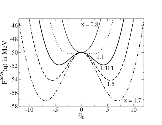
Figure 1: $\mathcal{F}^{\textrm{SPA}}$ at $T=0$ as a function of $q_{0}$ for different effective coupling constants $\kappa$.

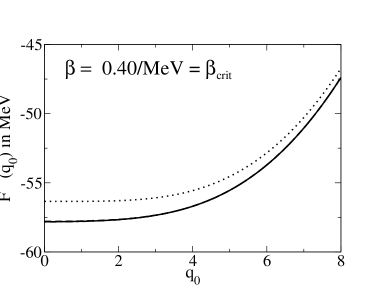
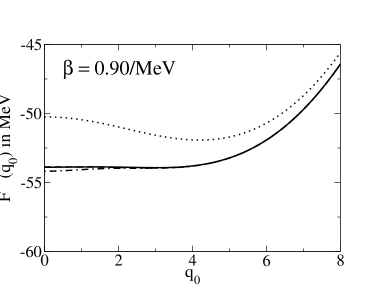
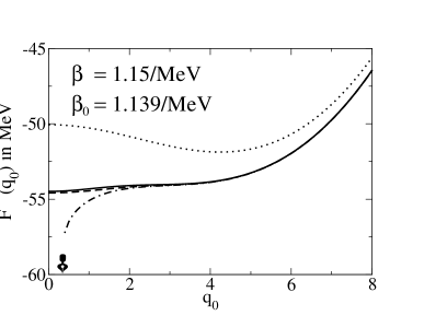
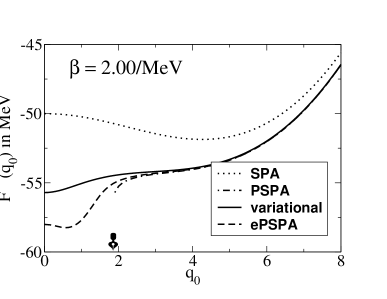
Figure 2: $\mathcal{F}^{\textrm{SPA}}$ and different approximations to the effective free energy $\mathcal{F}^{\textrm{eff}}$ of (4) for $\kappa=1.313$ as a function of $q_{0}$ at various temperatures. The inverse critical and crossover temperature are $\beta_{\textrm{crit}}=0.4~{}\textrm{MeV}^{-1}$ and $\beta_{0}=1.139~{}\textrm{MeV}^{-1}$ respectively. $\mathcal{F}^{\textrm{eff}}$ is an even function of $q_{0}$. The arrows point to the smallest $q_{0}$ where (at a given temperature) the PSPA still is formally applicable.

Also shown in Fig. 2 are the corrections to the SPA which one gains by the approximations to the $\mathcal{F}^{\textrm{eff}}$ of (4) described before. For these calculations the number $N$ of Fourier coefficients $q_{r}$ has been limited to $N=100$, and hence also for the products and sums in correction factors like (19) or (3). It has been checked that larger values of $N$ do not change the results anymore. Considerable corrections to the classical SPA are seen at any temperature for both the PSPA, the ePSPA as well as the variational approach. Up to $\beta=0.9~{}\textrm{MeV}^{-1}\approx 0.8\beta_{0}$ differences among them are hardly visible. The inverse crossover temperature for the PSPA lies at $\beta_{0}=1.139~{}\textrm{MeV}^{-1}$. At this temperature the sign change of the coefficient $\lambda_{1}$ takes place at the barrier top at $q_{0}=0$ of $\mathcal{F}^{\textrm{SPA}}$ and leads to a divergence of the $q_{1}$-integrals. For $\beta>\beta_{0}$ this pathologic region grows to larger $|q_{0}|$. Deviations between the ePSPA and the variational approach are clearly visible at $\beta=2~{}\textrm{MeV}^{-1}\approx 1.8\beta_{0}$.

It is remarkable that the effective free energy of the variational approach (fully drawn line in Fig. 2) shows only little structure in the barrier region of $\mathcal{F}^{\textrm{SPA}}$. This feature does not change qualitatively at even larger $\beta$ and is in agreement with the experience with the Feynman-Kleinert variational approach (FKV) [15, 27] if applied to a one-dimensional double-well potential: There at low temperatures in the approximation $W_{1}(x_{0})$ to the effective classical potential $W(x_{0})$ (which can be seen as special one-dimensional cases of the effective free energies $\mathcal{F}^{\textrm{var}}$ and $\mathcal{F}^{\textrm{eff}}$, respectively) no barrier exists anymore. In [28] Monte-Carlo simulations of the effective classical potential $W(x_{0})$ have been discussed for the same problem. It is reassuring that at small temperatures also such a $W(x_{0})$ was found flat in the barrier region.

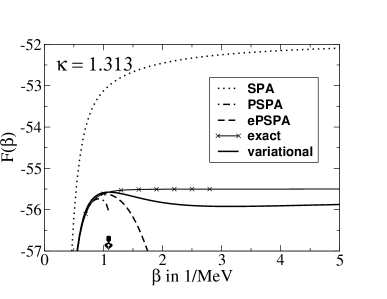
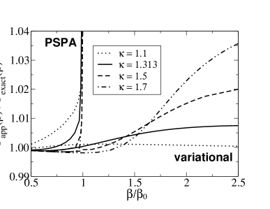
Figure 3: Left: Free energy of the total system in the LMGM as a function of $\beta$. The arrow points to the inverse crossover temperature $\beta_{0}$. Right: Comparison of the accuracy of the PSPA and the variational approach to the free energy of the LMGM.

Next we turn to the free energy (6) of the total system with the partition function calculated from (4). The quality of the different approximations are illustrated in Fig. 3. From the left panel it becomes evident that for an effective coupling constant of $\kappa=1.313$ the classical SPA is acceptable only at high temperatures (small $\beta$). In the regime $\beta<0.9~{}\textrm{MeV}^{-1}\approx 0.8\beta_{0}$ the PSPA improves this classical result by accounting for local RPA modes. A serious deficiency of the PSPA is its breakdown at $\beta=\beta_{0}=1.139~{}\textrm{MeV}^{-1}$. Even in a region below $\beta_{0}$ its results are no longer reliable. On the other hand the extension ePSPA of [12] behaves completely regular in the crossover region $\beta\approx\beta_{0}$. It can be used as a reasonable approximation up to $\beta\approx 1.2~{}\textrm{MeV}^{-1}\approx\beta_{0}$ but breaks down at still larger $\beta$. In contrast, the variational approach is applicable even at very low temperatures. There the relative error is of the order of 1% only.

Unfortunately, as can be seen from Fig. 3 the free energy $\mathcal{F}^{(4)}(\beta)$ of the variational approach is not a monotonously increasing function of $\beta$ as it should be according to the first law of thermodynamics. However, this deficiency is much worse for the PSPA and the ePSPA in a region $T>T_{0}$ of formal applicability just before the breakdown. To the best of our knowledge this problem has never been payed attention to in the literature on PSPA. Conversely, the free energy of our variational approach still is an increasing function in the crossover region, where that of the PSPA and the ePSPA already decrease. As we will explain below, there are indications that the pathological feature of $\mathcal{F}^{(4)}(\beta)$ which occurs at even lower temperatures is due to the truncation of the reference action and not a property of the variational approach itself. Also, it is seen that for $\beta>1.2~{}\textrm{MeV}^{-1}\approx\beta_{0}$ the variational free energy becomes smaller than the exact result. Although this behavior seems to be in contradiction to the restriction, in fact there is no violation of (24). To understand this, one should notice that the inequality (21) itself is valid for the truncated action $s_{\textrm{E}}^{(4)}$ as well. Of course, this inequality does not necessarily hold in case that different actions are used on both sides, say like $s_{\textrm{E}}$ on the left and $s_{\textrm{E}}^{(4)}$ on the right. Hence, different to (24) no inequality can be written down between the approximation $\mathcal{F}^{(4)}(\beta)\approx\mathcal{F}^{\textrm{var}}(\beta)$ and the exact free energy $\mathcal{F}(\beta)$.

We have been able to reproduce a similar behavior of the free energy using the FKV of [15, 27] to calculate the partition function of a particle of mass $M$ moving in a one-dimensional double-well potential $V(x)=-ax^{2}+(1-a)x^{6}$ (where $0<a<1$) with anharmonicity of higher than fourth order. Taking into account the inharmonic terms to all orders the free energy of the FKV indeed is a monotonously increasing function of $\beta$ and the inequality (24) is fulfilled by the variational approach for all temperatures. A truncation of the Euclidean action after the fourth order in the $q_{r}$ leads to a free energy that is smaller than the exact result and becomes decreasing at low temperatures. This observation indicates that also the unphysical decrease of the free energy $\mathcal{F}^{(4)}(\beta)$ in the left panel of Fig. 3 does not reflect a deficiency of the variational approach as such, rather it is an artefact of the truncation of the reference action.

In the right panel of Fig. 3 the accuracy of the PSPA and the variational approach is tested at the example of the free energy (6) by showing the ratio of the approximate results to the exact one. This is done for different effective coupling constants $\kappa>1$. It is observed that within its range of applicability, which is to say for $\beta<\beta_{0}$, the accuracy of the PSPA increases with increasing $\kappa$. This may be traced back to the fact that the barrier height of the effective free energy $\mathcal{F}^{\textrm{SPA}}$ at $T=0$ grows with $\kappa$, see again Fig. 1. However, the larger the barrier the smaller the probability for quantum tunneling and, hence, the less important are fluctuations of large scale. However, when these fluctuations become more and more localized their treatment as local RPA modes becomes better and better. Contrary to the PSPA, the accuracy of the variational approach becomes worse the larger the barrier height. As can be seen from the right panel of Fig. 3 this feature is more pronounced for larger $\beta$. In the range $0\leq\beta<\beta_{0}$, on the other hand, the results of the variational approach are better than those of the PSPA. One should recall, perhaps, that nature of the inharmonic terms of $\mathcal{F}^{\textrm{SPA}}$ taken into account by the variational approach still is based on a local approximation. It does not base on a large scale mode like the one necessary to describe quantum tunneling correctly. These findings are in agreement with the results of the FKV for the case of the one-dimensional double-well potential: There, it has been observed that for high barriers the FKV is unable to describe the splitting of low lying levels due to tunneling correctly [15].

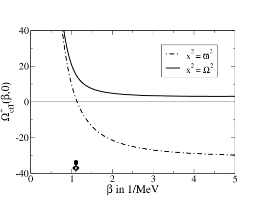
Figure 4: Comparison of the “stiffnesses” $\Omega_{\textrm{eff}}^{2}$ of $s_{\textrm{E}}^{\textrm{PSPA}}$ and $s_{\Omega}^{q_{0}}$ in $q_{1}$-direction defined in (35) using the RPA-frequency $\varpi$ and the variational parameter $\Omega$, respectively. The arrow points to the inverse crossover temperature. The effective coupling strength is $\kappa=1.313$.

An interesting question is why the variational approach does not suffer a real breakdown. For an answer it is useful to look at the quantities

$$\Omega_{\textrm{eff}}^{2}(\beta,q_{0})=\left(\frac{2\pi}{\hbar\beta}\right)^{2}+x^{2}(\beta,q_{0})\qquad\textrm{with}\qquad x^{2}(\beta,q_{0})=\begin{cases}\varpi^{2}(\beta,q_{0})\\[4.0pt] \Omega^{2}(\beta,q_{0})\,.\end{cases}$$ (35)

They largely define the stiffnesses of $s_{\textrm{E}}^{\textrm{PSPA}}$ and $s_{\Omega}^{q_{0}}$ in $q_{1}$-direction (see (25) and mind $\nu_{1}=2\pi/\hbar\beta$ as well as the fact that the product over $\mu$ reduces to a single factor in the LMGM). After the manipulations described in Sect. 2 and 3, $\Omega_{\textrm{eff}}^{2}$ contributes to the denominators of the correction factors (19) and (3). Fig. 4 shows the $\Omega_{\textrm{eff}}^{2}$ of (35) as a function of $\beta$ and for $q_{0}=0$ (where the square of the RPA-frequency $\varpi^{2}$ becomes negative for $\beta>\beta_{\textrm{crit}}$ and takes on the largest absolute value). For $x^{2}=\varpi^{2}$ the $\Omega_{\textrm{eff}}^{2}$ becomes negative at the inverse crossover temperature $\beta_{0}$ and the $q_{1}$-integral needed in (8) diverges at larger $\beta$. Consequently, the formula (19), which has been derived under the condition that all $q_{r}$-integrals converge, is no longer valid under these circumstances. On the other hand using $x^{2}=\Omega^{2}$ garanties $\Omega_{\textrm{eff}}^{2}$ to be strictly positive. As now all $q_{r}$-integrals appearing in (20) are of Gaussian type, the correction factor (3) of the variational approach is well defined for all $\beta$. As a result of this feature the effective free energy $\mathcal{F}^{\textrm{var}}$ shows much less structure than $\mathcal{F}^{\textrm{PSPA}}$, as already mentioned in connection with Fig. 2.

Further tests of the accuracy of the different approximations may be done for the internal energy $\mathcal{E}(\beta)=-\partial\,\textrm{ln}\mathcal{Z}(\beta)/\partial\beta$ [13] of the total system or for the specific heat $\mathcal{C}(\beta)=\beta^{2}\,\partial^{2}\,\textrm{ln}\mathcal{Z}(\beta)/\partial\beta^{2}$. We concentrate on the latter for $\kappa>1$ here.

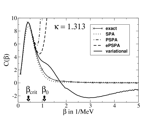
Figure 5: The specific heat of the LMGM as a function of $\beta$ in various approximations. The arrows point to the inverse critical temperature $\beta_{\textrm{crit}}$ where the barrier in $\mathcal{F}^{\textrm{SPA}}$ starts to build up at $q_{0}=0$ and the inverse crossover temperature $\beta_{0}$.

In Fig. 5 the classical SPA is seen to deliver a qualitatively correct behavior of the specific heat at all temperatures. For $\beta\approx\beta_{\textrm{crit}}$ it under-estimates the exact result by about 10%. At these smaller $\beta$, however, the PSPA and the ePSPA supply much better approximations. But they cease to be reliable already far below their formal limits of applicability at $\beta_{0}$ and $2\beta_{0}$ respectively. There the variational approach leads to much better results, at least for not too large values of $\beta$. For $\beta\gtrsim 1.7~{}\textrm{MeV}\approx 1.5\beta_{0}$, on the other hand, it leads to negative values. Let us note that this problem is much less pronounced for $\kappa<1$ and closely related to the appearance of positive curvatures of the $\mathcal{F}(\beta)$ shown in the left panel of Fig. 3. The exact origin of this unphysical behavior is still unclear and must be investigated further. Perhaps and similar to the (apparent) violation of (24) the effect might be related to the truncation of the expansion (9) of the Euclidean action $\langle\delta s_{\textrm{E}}\rangle_{\Omega}^{q_{0}}$ at fourth order in (30). However, studying analog truncations in one-dimensional calculations within the FKV of [15, 27], so far we have not found a similar behavior of the specific heat even for systems with strong inharmonic terms. Therefore the origin of the negative specific heat in Fig. 5 will have to be investigated further.

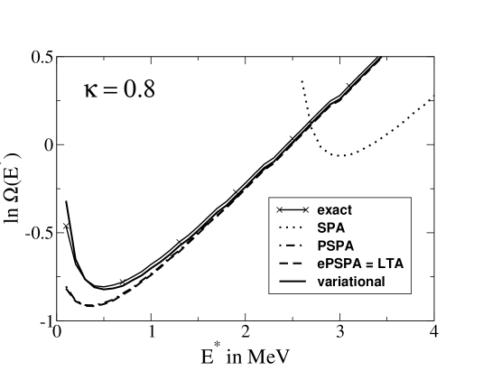
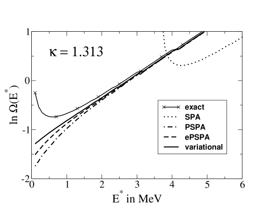
Figure 6: Logarithmic representation of the Darwin-Fowler approximation to the level density as function of the excitation energy $E^{*}=E-E_{0}$ in various approximations. Whereas for $\kappa=0.8$ no barrier is present in $\mathcal{F}^{\textrm{SPA}}$, for $\kappa=1.313$ it builds up at $\beta=\beta_{\textrm{crit}}$.

One prominent application of the SPA or the PSPA has been the calculation of the level density $\rho$ of finite, interacting many body systems beyond the independent particle model [7, 8, 9, 21]. In Fig. 6 this level density is shown as function of the excitation energy $E^{*}=E-E_{0}$. The calculations have been performed with the Darwin-Fowler method (i.e. a saddle point approximation to the inverse Laplace transform from $\mathcal{Z}(\beta)$ to $\rho(E^{*})$, see e.g. [17]). For the case of non-positive heat capacities this becomes problematic as then the equation $E=\mathcal{E}(\beta)=-\partial\,\textrm{ln}\mathcal{Z}(\beta)/\partial\beta$ no longer has unique solutions. In our application we have concentrated on the one with smallest $\beta$, simply because the other one lies in that regime of $\beta$ where $\mathcal{E}(\beta)$ has a positive slope, implying $\mathcal{C}(\beta)<0$. For excitations $E^{*}$ above about $15~{}\textrm{MeV}$ (not shown in the plots) all approximations are in good agreement with the Darwin-Fowler calculation which is based on the exact partition function $\mathcal{Z}(\beta)$. At smaller $E^{*}$, however, the level density of the classical SPA is qualitatively wrong. Here, all other approximations lead to considerable improvements over the SPA result. When the $\mathcal{F}^{\textrm{SPA}}$ has no barrier, like for $\kappa=0.8$ (see Fig. 1), the PSPA and ePSPA can hardly be distinguished from each other and show a qualitatively correct behavior. On the other hand, for $\kappa=1.313$, which is to say when the $\mathcal{F}^{\textrm{SPA}}$ exhibits a barrier for low temperature (see Fig. 2), both the PSPA as well the ePSPA do not reproduce correctly the behavior of the calculation using the full $\mathcal{Z}(\beta)$. Nevertheless, the ePSPA shows a certain improvement over the PSPA. For $\kappa=0.8$ the variational approach reproduces perfectly well the calculation done for the exact $\mathcal{Z}(\beta)$. For the case of a barrier with $\kappa=1.313$ one is in the situation discussed above where within our present approximation the specific heat becomes negative above a certain value of $\beta$, see Fig.5. Although a clear improvement over the ePSPA is seen, the present version of the variational approach is not capable of reproducing the qualitative behavior right at small $E^{*}$. Finally we like to note that for $E^{*}$ below about $0.3-0.5$ MeV the Darwin-Fowler method itself becomes questionable. This feature is in accord with the fact that the heat capacity approaches zero at about $\beta\simeq 2~{}\text{MeV}^{-1}$.

5 Discussion

A variational approach to the partition function of a finite, interacting many body system has been developed and applied to the exactly solvable LMGM. It has been shown that for thermodynamic quantities like the free energy or the level density it delivers quite accurate results. This is especially important as the variational approach can formally be applied without any problems in the low temperature regime $\beta>\beta_{0}$, where the PSPA breaks down. In the crossover range $\beta\approx\beta_{0}$ the variational approach considerably improves the approximations used so far.

At very low temperatures there is still some deviation of the variational from the exact results, which may be explained as follows: Also the variational approach starts from a static auxiliary field and takes into account small quantum fluctuations: $q(\tau)\approx q_{0}$. At very low temperatures, however, large scale fluctuations like quantum tunneling cannot be neglected. To include such effects the full nonlinearity of the problem must be considered. For interacting many body problems this is still an open problem.

The range of applicability of the method proposed is not limited to problems of nuclear physics. Superconductivity in ultra-small metallic grains [2] is a prime example for possible applications in condensed matter physics, where up to now the path integral approach has been limited to the PSPA [4].

Unfortunately, the benefits gained through the variational approach must be payed for by a significantly larger computational effort. The two quantities that most influence the computation time are the number $N$ of Fourier coefficients $q_{r}$ (where $r=1\ldots N$) and the dimension $m$ of the space spanned by the variational parameters $\Omega_{\mu}^{2}$ (where $\mu=1\ldots m$ and $1\leq m\leq M$). With respect to the Fourier coefficients the computation time for the PSPA and the ePSPA of [12] is limited by the calculation of the $N$ coefficients $\lambda_{r}$ of (17) (and the three coefficients $\rho_{11-2}$, $\rho_{-1-12}$ of (11) and $\sigma_{11-1-1}$ of (12) in the case of ePSPA). In contrast, for the variational approach in addition all the $N^{2}$ coefficients $\sigma_{rs-r-s}$ must be evaluated according to the formulas given in [12, 13]. In the case of an extension of the expansion (9) to order $2n$ even $N^{n}$ coefficients would have to be calculated. Please have in mind that the one-dimensional analog [14, 15, 27] of the method proposed here does not suffer from this complication. There the expansion coefficients can be read off directly from the Taylor expansion of the underlying potential $V(x)$.

The computation time for the variational procedure required for minimizing (23) with (3) is given by the task of finding the absolute minimum of a scalar function in an $m$-dimensional space. As this effort strongly depends on the underlying function, no strict statement is possible concerning the number of necessary operations. Nevertheless it is intuitively clear that this number strongly increases with the dimension $m$ of the corresponding space. Therefore, the choice (a) in (28) and (26) may imply serious drawbacks. On the other hand, the choice (b) shows the way out of this problem. The essential idea is to restrict the variational procedure to the lowest-lying mode $\varpi_{1}^{2}$ that leads to the breakdown of the PSPA and contributes most to the product of (17). A similar philosophy is exploited in [29] in order to be able to introduce dissipative effects. In cases where the restriction of the number of the variational parameters to $m=1$ is not good enough, it should be possible to introduce variational parameters $\Omega_{\mu}^{2}$ for a small number $m\ll M$ of such modes only and use the RPA frequencies $\varpi_{\mu}^{2}$ for the rest.

Appendix A Evaluation of the averages

A.1 Second order contributions

Using the definitions (26)–(28) the second order contribution to the average necessary on the right hand side of (21) is

$$\langle s_{\textrm{E}}^{\textrm{PSPA}}-s_{\Omega}^{q_{0}}\rangle_{\Omega}^{q_{0}}$$ (36)

$$= \frac{1}{\zeta_{\Omega}^{q_{0}}}\int\prod_{s>0}\frac{\beta}{\pi|k|}\,d\textrm{Re}(q_{s})d\textrm{Im}(q_{s})\,\exp\left(-\frac{\beta}{|k|}\sum_{s>0}\Lambda_{s}\cdot\left(\textrm{Re}^{2}(q_{s})+\textrm{Im}^{2}(q_{s})\right)\right)\times$$

$$\frac{\hbar\beta}{|k|}\sum_{r>0}\Pi_{r}\Lambda_{r}\,\left(\textrm{Re}^{2}(q_{r})+\textrm{Im}^{2}(q_{r})\right)$$

$$= \frac{\hbar\beta}{|k|}\sum_{r>0}\Pi_{r}\Lambda_{r}^{2}\times$$

$$\int\frac{\beta}{\pi|k|}\,d\textrm{Re}(q_{r})d\textrm{Im}(q_{r})\ \exp\left(-\frac{\beta}{|k|}\,\Lambda_{r}\cdot\left(\textrm{Re}^{2}(q_{r})+\textrm{Im}^{2}(q_{r})\right)\right)\,\left(\textrm{Re}^{2}(q_{r})+\textrm{Im}^{2}(q_{r})\right)$$

$$= \hbar\sum_{r>0}\Pi_{r}\,.$$

Here in the second identity we have carried out all Gaussian integrals with $s\neq r$. In the third identity the remaining non-Gaussian integrals are evaluated. Note that the sum in the final expression is convergent due to the fact that the denominator of $\Pi_{r}$ is two orders higher in $\nu_{r}=(2\pi/\hbar\beta)\,r$ than the numerator (see (28)).

A.2 Fourth order contributions

Due to symmetry arguments in fourth order the only contributing terms read

$$\langle\delta s_{\textrm{E}}^{(4)}\rangle_{\Omega}^{q_{0}}$$ (37)

$$= \frac{1}{\zeta_{\Omega}^{q_{0}}}\,\int\prod_{t>0}\frac{\beta}{\pi|k|}\,d\textrm{Re}(q_{t})d\textrm{Im}(q_{t})\,\exp\left(-\frac{\beta}{|k|}\sum_{t>0}\Lambda_{t}\cdot\left(\textrm{Re}^{2}(q_{t})+\textrm{Im}^{2}(q_{t})\right)\right)\times$$

$$\frac{\hbar\beta}{|k|}\sum_{r,s>0}\sigma_{rs-r-s}\,(\textrm{Re}^{2}(q_{r})+\textrm{Im}^{2}(q_{r}))\,(\textrm{Re}^{2}(q_{s})+\textrm{Im}^{2}(q_{s}))$$

$$= \frac{\hbar\beta}{|k|}\sum_{r,s>0}\sigma_{rs-r-s}\,\Lambda_{r}\,\Lambda_{s}\times$$

$$\int\frac{\beta}{\pi|k|}\,d\textrm{Re}(q_{r})d\textrm{Im}(q_{r})\ \exp\left(-\frac{\beta}{|k|}\,\Lambda_{r}\cdot\left(\textrm{Re}^{2}(q_{r})+\textrm{Im}^{2}(q_{r})\right)\right)\left(\textrm{Re}^{2}(q_{r})+\textrm{Im}^{2}(q_{r})\right)$$

$$\int\frac{\beta}{\pi|k|}\,d\textrm{Re}(q_{s})d\textrm{Im}(q_{s})\ \exp\left(-\frac{\hbar\beta}{|k|}\,\Lambda_{s}\cdot\left(\textrm{Re}^{2}(q_{s})+\textrm{Im}^{2}(q_{s})\right)\right)\left(\textrm{Re}^{2}(q_{s})+\textrm{Im}^{2}(q_{s})\right)$$

$$= \frac{\hbar|k|}{\beta}\sum_{r,s>0}\sigma_{rs-r-s}\,\frac{1}{\Lambda_{r}}\,\frac{1}{\Lambda_{s}}\,.$$

The quantities $\Lambda_{r}$ defined in (26) have been used. The special case $r=s$ is included in (37). Note that for constant coefficients $\sigma_{rs-r-s}$ the sum would not converge. Only the behavior (31) garanties convergence of the sum.

References

- [1] H. Attias and Y. Alhassid, Nucl. Phys. A 625, 565 (1997).
- [2] D. Ralph, C. Black, and M. Tinkham, Phys. Rev. Lett. 74, 3241 (1995); C. Black, D. Ralph, and M. Tinkham, Phys. Rev. Lett. 76, 688 (1996); D. Ralph, C. Black, and M. Tinkham, Phys. Rev. Lett. 78, 4087 (1997).
- [3] F. Braun, J. v. Delft, D. Ralph and M. Tinkham, Phys. Rev. Lett. 79, 921 (1997); F. Braun, J. v. Delft, Phys. Rev. Lett. 81, 4712 (1998); F. Braun, J. v. Delft, Phys. Rev. B 59, 9527 (1999).
- [4] R. Rossignoli, J.P. Zagorodny, and N. Canosa, Phys. Lett. A 258, 188 (1999); R. Rossignoli, N. Canosa, P. Ring, Ann. Phys. 275, 1 (1999); N. Canosa and R. Rossignoli, Phys. Rev. B 62, 5886 (2000); R. Rossignoli and N. Canosa, Phys. Rev. B 63, 134523 (2001).
- [5] J. W. Negele and H. Orland, Quantum Many-Particle Systems (Addison-Wesley, Reading, MA, 1988).
- [6] B. Mühlschlegel, D. Scalapino, and R. Denton, Phys. Rev. B 6, 1767 (1972).
- [7] Y. Alhassid and J. Zingman, Phys. Rev. C 30, 684 (1984).
- [8] B. Lauritzen, P. Arve and G.F. Bertsch, Phys. Rev. Lett. 61, 2835 (1988).
- [9] G. Puddu, P. F. Bortignon, and R. A. Broglia, Ann. Phys. (San Diego) 206, 409 (1991).
- [10] R. Rossignoli and N. Canosa, Phys. Lett. B 394, 242 (1997).
- [11] R. Rossignoli and P. Ring, Nucl. Phys. A 633, 613 (1998).
- [12] C. Rummel and J. Ankerhold, Eur. Phys. J. B 29, 105 (2002).
- [13] C. Rummel, Ph.D. thesis, Technische Universität München, 2004.
- [14] R. Giachetti and V. Tognetti, Phys. Rev. Lett. 55, 912 (1985); R. Giachetti and V. Tognetti, Phys. Rev. B 33, 7647 (1986).
- [15] R. P. Feynman and H. Kleinert, Phys. Rev. A 34, 5080 (1986).
- [16] H. J. Lipkin, N. Meshkov, and A. J. Glick, Nucl. Phys. 62, 188 (1965).
- [17] A. Bohr and B. R. Mottelson, Nuclear Structure (Benjamin, London, 1975), Vol. 1.
- [18] G. Puddu, Phys. Rev. C 44, 905 (1991).
- [19] N. Canosa and R. Rossignoli, Phys. Rev. C 56, 791 (1997).
- [20] C. Rummel, H. Hofmann, Phys. Rev. E 64, 066126 (2001).
- [21] B. K. Agrawal and A. Ansari, Phys. Lett. B 421, 13 (1998).
- [22] H. Hofmann, Phys. Rep. 284 (4&5), 137 (1997).
- [23] H. Grabert and U. Weiss, Phys. Rev. Lett. 53, 1787 (1984); H. Grabert, P. Olschowski, and U. Weiss, Phys. Rev. B 36, 1931 (1987).
- [24] P. Hänggi, P. Talkner, and M. Borkovec, Rev. Mod. Phys. 62, 251 (1990).
- [25] U. Weiss, Quantum Dissipative Systems (World Scientific, Singapore, 1993).
- [26] S. K. You, C. K. Kim, K. Nahm, and H. S. Noh, Phys. Rev. C 62, 045503 (2000).
- [27] H. Kleinert, Pathintegrals in Quantum Mechanics, Statistics and Polymer Physics (World Scientific, Singapore, 1990).
- [28] W. Jahnke and H. Kleinert, Chem. Phys. Lett. 137, 162 (1987).
- [29] C. Rummel and H. Hofmann, nucl-th/0407092