Abstract

The renormalization of EFT for nucleon-nucleon scattering in nonperturbative regimes is investigated in a compact parametrization of the $T$-matrix. The key difference between perturbative and nonperturbative renormalization is clarified. The underlying theory perspective and the ’fixing’ of the prescriptions for the $T$-matrix from physical boundary conditions are stressed.

1

In recent years, the effective field theory (EFT) method has become the main tool to deal with various low energy processes and strong interactions in the nonperturbative regime. Beginning from Weinberg’s seminal works[1], this method has been extensively and successfully applied to the low energy nucleon systems[2]. As an EFT parametrizes the high energy details in a simple way, there appear severe UV divergences (or ill-definedness) and more undetermined constants that must be fixed somehow. Owing to the nonperturbative nature, the EFT for nuclear forces also becomes a theoretical laboratory for studying the nonperturbative renormalization and a variety of renormalization (and power counting) schemes have been proposed[3, 4, 5, 6, 7, 8, 9, 10, 11, 12, 13]. However, a complete consensus and understanding on this important issue has yet not been reached. Though the EFT philosophy is very natural, but its implementation requires discretion (in parametrizing the short distance effects)[14]. In particular, as will be shown below, the nonperturbative context impedes the implementation of conventional subtraction renormalization, and some regularization/renormalization (R/R) prescription might even fail the EFT method or physical predictions[5, 9, 15], unlike in the perturbative case[16].

In this short report, we shall revisit the problem without specifying the R/R scheme (we only need that the renormalization is done) to elucidate the key features for the implementation of R/R in nonperturbative regime, and various proposals could be compared and discussed. Then the key principles that should be followed are suggested as the first steps in such understandings.

2

The physical object we are going to investigate is the transition matrix $T$ for nucleon-nucleon scattering processes at low energies,

$$N({\bf p})+N({\bf-p})\rightarrow N({\bf p}^{\prime})+N({\bf-p}^{\prime}),$$ (1)

which satisfies the Lippmann-Schwinger (LS) equation in partial wave formalism,

$$T_{ll^{\prime}}(p^{\prime},p;E)=V_{ll^{\prime}}(p^{\prime},p)+\sum_{l^{\prime\prime}}\int\displaystyle\frac{kdk^{2}}{(2\pi)^{2}}V_{ll^{\prime\prime}}(p^{\prime},k)G_{0}(k;E^{+})T_{l^{\prime\prime}l^{\prime}}(k,p;E),$$

$$G_{0}(k;E^{+})\equiv\frac{1}{E^{+}-k^{2}/(2\mu)},\ \ E^{+}\equiv E+i\epsilon,$$ (2)

with $E$ and $\mu$ being respectively the center energy and the reduced mass, ${\bf p}$ (${\bf p}^{\prime}$) being the momentum vector for the incoming (outgoing) nucleon, and $p^{\prime}=|{\bf p}^{\prime}|$, $p=|{\bf p}|$. The potential $V(p^{\prime},p)$ can be systematically constructed from the $\chi$PT[17, 1]. We remind that the constructed potential is understood to be finite first, as ’tree’ vertices in the usual field theory terminology.

Now let us transform the above LS equation into the following compact form as a nonperturbative parametrization of $T$-matrix, we temporarily drop all the subscripts that labelling the status of the finiteness and divergence:

$$T^{-1}=V^{-1}-{\mathcal{G}},$$ (3)

where ${\mathcal{G}}\equiv V^{-1}\{\int\frac{kdk^{2}}{(2\pi)^{2}}VG_{0}T\}T^{-1}$ is obviously a nonperturbative quantity. Here $V$, $T$ and therefore ${\mathcal{G}}$ are momenta dependent matrix in angular momentum space. In field theory language, ${\mathcal{G}}$ contains all the ’loop’ processes generated by the 4-nucleon vertex $V$ joined by nucleon (and antinucleon) lines[7]. This nonperturbative parametrization clearly separates $V$ (Born amplitude) from ${\mathcal{G}}$ (all the iterations or rescatterings), and on-shell ($p^{\prime}=p=\sqrt{2\mu E}$) unitarity (nonperturbative relation) of $T$ is automatically satisfied here thanks to the on-shell relation between the $K$-matrix and $T$-matrix[18]

$$T^{-1}_{os}=K^{-1}_{os}+i\mu\frac{\sqrt{2\mu E}}{2\pi},$$ (4)

Using Eq.( 3) we have

$${\mathcal{G}}_{os}=V_{os}^{-1}-K_{os}^{-1}-i\mu\frac{\sqrt{2\mu E}}{2\pi}.$$ (5)

Any approximation to the quantity ${\mathcal{G}}$ leads to a nonperturbative scheme for $T$.

Since the on-shell $T$-matrix must be physical, then for general potential functions this nonperturbative parametrization leads to the following obvious but important observations in turn: (I) it is impossible to renormalize ${\mathcal{G}}$ through conventional perturbative counter terms in $V$ (we will demonstrate this point shortly), i.e., they have to be separately renormalized; (II) the perturbative pattern of the scheme dependence for transition matrix or physical observables[16] breaks down in the nonperturbative contexts like Eq.( 3); (III) the R/R for $V$ and ${\mathcal{G}}$ must be so performed that the on-shell $T$-matrix satisfies physical boundary conditions (bound state and/or resonance poles[19, 7], scattering lengths or phase shifts[20], etc.), i.e, $V$ and ${\mathcal{G}}$ are ’locked’ with each other; (IV) due to this ’locking’, the validity of the EFT power counting in constructing $V$ also depends on the R/R prescription for ${\mathcal{G}}$, i.e., the power counting of $V$ could be vitiated by the R/R prescription for ${\mathcal{G}}$ which is performed afterwards. This explains why there are a lot of debates on the consistent power counting schemes for constructing $V$. Point (III) is in fact what most authors actually did or is implicit in their treatments. we will return to these points later.

To be more concrete or to demonstrate the first point (observation (I)), let us consider the case without mixing ($l=l^{\prime}$) for simplicity. Then the matrices become diagonal and only energy dependent due to on-shell condition, we have the following simple form of nonperturbative parametrization (from now on we will drop the subscript ”os” for on-shell),

$$\frac{1}{T_{l}(E)}=\frac{1}{V_{l}(E)}-{\mathcal{G}}_{l}(E),$$ (6)

where ${\mathcal{G}}_{l}(E)=\frac{(\int\frac{kdk^{2}}{(2\pi)^{2}}VG_{0}T)_{l}(E)}{V_{l}(E)T_{l}(E)}$. In perturbative formulation, all the divergences are removed order by order before the loop diagrams are summed up. Here, in Eq.( 6) (or Eq.( 3)), the renormalization are desired to be performed on the compact nonperturbative parametrization. After $V$ is calculated and renormalized within $\chi$PT, the task is (a) to remove the divergence or ill-definedness in ${\mathcal{G}}_{l}(E)$ and (b) to make sure that the renormalized quantities ($V^{(R)}_{l}(E)$ and ${\mathcal{G}}^{(R)}_{l}(E)$) lead to a physical $T$-matrix. The most important one is (b), namely the $T$-matrix obtained must possess reasonable or desirable physical behaviors after removing the divergences. Technically, this amounts to a stringent criterion for the R/R prescription in use: the functional form of ${\mathcal{G}}_{l}(E)$ could not be altered, only the divergent parameters (coefficients) get ’replaced’ by finite ones.

Now let us suppose ${\mathcal{G}}_{l}$ could be renormalized by introducing counter terms. Within this parametrization of Eq.( 6), the potential $V$ appears as the only candidate to bear counter terms, then from Eq.( 6) we would have

$${\mathcal{G}}^{(R)}_{l}(E)={\mathcal{G}}^{(B)}_{l}(E)+\frac{1}{V^{(R)}_{l}(E)}-\frac{1}{V^{(R)}_{l}(E)+\delta V_{l}(E)},$$ (7)

where the superscripts $(R)$ and $(B)$ refer to ’renormalized’ and ’bare’, $\delta V_{l}$ denotes the additive counter terms and $V^{(B)}_{l}(E)\equiv V^{(R)}_{l}(E)+\delta V_{l}(E)$.

From the definition below Eq.( 3), ${\mathcal{G}}$ must take the following form which is no less complicated than a nonpolynomial function in $p(=\sqrt{2\mu E})$,

$${\mathcal{G}}^{(B)}_{l}(E)=\frac{\int\frac{d^{3}k}{(2\pi)^{3}}V_{l}(p,k)G_{0}(k;E^{+})T_{l}(k,p;E)}{V_{l}(E)T_{l}(E)}=\frac{N^{(B)}_{l}(p)}{D^{(B)}_{l}(p)}-\frac{\mu}{2\pi}ip,$$ (8)

with $N^{(B)}_{l}(p),D^{(B)}_{l}(p)$ being at least two nontrivial divergent or ill-defined polynomials. With this parametrization, Eq.( 7) becomes

$${\mathcal{G}}^{(R)}_{l}(E)=\frac{N^{(B)}_{l}(p)V^{(R)}_{l}(E)V^{(B)}_{l}(E)+D^{(B)}_{l}(p)\delta V_{l}(E)}{D^{(B)}_{l}(p)V^{(R)}_{l}(E)V^{(B)}_{l}(E)}-\frac{\mu}{2\pi}ip=\frac{N^{(R)}_{l}(p)}{D^{(R)}_{l}(p)}-\frac{\mu}{2\pi}ip.$$ (9)

Note that in the divergent or ill-defined fraction $\frac{N^{(B)}_{l}(p)V^{(R)}_{l}(E)V^{(B)}_{l}(E)+D^{(B)}_{l}(p)\delta V_{l}(E)}{D^{(B)}_{l}(p)V^{(R)}_{l}(E)V^{(B)}_{l}(E)}$ only $V^{(R)}_{l}(E)$ is finite. Then except for the simplest form of $V_{l}(E)$ (= $C_{0}$, see, e.g., Ref.[2]), it is impossible to obtain a nontrivial and finite fraction out of the this divergent fraction with whatever counter terms $\delta V_{l}(E)$, i.e., it is impossible to remove the divergences in the numerator and the denominator at the same time with the same counter terms as in Eq.( 9). Examples for nonperturbative divergent fractions could be found in Ref.[5]. Even by chance ${\mathcal{G}}$ is finite, then its functional form in terms of physical parameters ($E,p$) must have been altered (often oversimplified) after letting the cutoffs go infinite. For channels with mixing, with $V_{l}$ and ${\mathcal{G}}_{l}$ becoming $2\times 2$ matrices, all the preceding deductions still apply. Thus within nonperturbative regime the counter term (via potential) renormalization of $T$-matrix fails, that is, ${\mathcal{G}}$ must be separately renormalized–the first observation given above is demonstrated as promised. The other observations follow easily.

What we have just shown does not mean that the counter term fails at any rate. The above arguments showed that the counter term could not successfully renormalize the nonperturbative $\mathcal{G}$ or $T$-matrix except they are introduced before the corresponding infinite perturbative series are summed up or before all parts of the nonperturbative objects are put together and ’installed’, say, before the corresponding Schrödinger equation is solved. It is well known that the Schrödinger equation approach[10] or similar[13] is intrinsically nonperturbative, therefore the counter terms introduced there (as parts of the potential operators) ARE nonperturbative in the sense that they enter before the $T$-matrix or phase shifts are finally derived, or equivalently, they must ’enter’ before the perturbative series are summed up. So there is no contradiction between our conclusion here and that in Ref.[10]. In fact they are in complete harmony and our conclusion above turns out to be also supporting the Schrödinger equation approach for renormalizing nucleon-nucleon scattering. Thus our discussions above are helpful to clarify the difference between perturbative and nonperturbative renormalization or to remove some mists or controversies around the renormalization of EFT for nucleon-nucleon scattering.

To make our language more concise, we would temporarily call the counter terms ’endogenous’ to an object if they must enter before all the necessary calculations on the interested object are done, and ’exogenous’ otherwise.

3

Therefore the renormalization in nonperturbative regime have to be implemented either with ’endogenous’ counter terms (e.g.,[10]) or otherwise (e.g., like in Refs.[12, 13]). To proceed we recall the conceptual foundation for EFT method: there must be a complete theory underlying all the low energy EFTs. Suppose we could compute the $T$-matrix in the underlying theory, then in the low energy limit, we should obtain a finite matrix element parametrized in terms of EFT coupling constants and certain finite constants arising from the limit. It is these constants that we are after. In the ill-defined EFT frameworks, a R/R or subtraction prescription is employed to ’retrieve’ the finite constants. As we have seen the failure of the counter term subtraction at the potential or vertex level in nonperturbative parametrization, the renormalization must be otherwise implemented. A prompt choice is the subtraction at the integral level, and the counter term formalism is dismissed from the underlying theory point of view. In this sense, the formal consistency issue of Weinberg power countings[7, 2] is naturally dissolved without resorting to other means, and the real concern is the renormalization instead of power counting rules. This resolution is in fact just a paraphrase of the fourth observation in section two (point (IV)): a consistent power counting could be vitiated by the afterward renormalization procedures such as those using exogenous counter terms.

If the ill-definedness only originates from the local part of the potential, the integral level subtraction is OK as the divergent integrals can be cleanly isolated[8, 12]. For the more interesting cases with general pion-exchange contributions, such clean isolation seems impossible, which leads some authors to perturbative approach (KSW[7]), but the convergence is shown to be slow[7, 2] and the KSW power counting also bears some problems[10]. Due to such difficulties, the regularization schemes with finite cutoffs or parameters have also been adopted to keep the investigations nonperturbative[3, 4, 6, 10], which have to be numerical. In such approaches certain sort of ’fitting to data’ is incorporated in one way or the other, this is what we stressed in section two. There recently appears a new approach that constructs the nonperturbative $T$-matrix from the KSW approach[11], where again certain sort of fitting is crucial there.

Then it is clear that the main obstacle is the severe regularization dependence in nonperturbative regime. If we could parametrize all the ill-definedness in ambiguous but finite expressions, then the obstacle would disappear and the only task is to fix the ambiguities. Otherwise, any theoretical judgement just based on one regularization scheme is unwarranted or ungrounded unless it is justified in various schemes [9, 22]. The importance of regularization in nonperturbative regime could also be seen in the following way: For any R/R prescription in nonperturbative regimes to be able to ’reproduce’ such ’true’ $T$-matrix obtained from underlying theory, the regularization in use should at least reproduce the same nonperturbative functional expression as that given in underlying theory, with certain constants being adjustable, otherwise the ’true’ functional expression could not be approached since exogenous counter terms, as we have shown above, could not be effected in nonperturbative parametrization. Alternatively, the foregoing arguments could be interpreted as a call for a devise of a new nonperturbative framework where endogenous counter terms could be naturally incorporated.

Our parametrization also points towards a new technical direction for the nonperturbative determination of the $T$-matrix: to focus on the calculation of ${\mathcal{G}}_{l}(E)$. The relevance of R/R in ${\mathcal{G}}$ can be made clearer in the low energy expansion of ${\mathcal{G}}$ (Padé or Taylor) since it is necessarily a function of the center energy ($E$) or on-shell momentum ($p$):

$$Re({\mathcal{G}}_{l}(p))|_{\texttt{Pad\'{e}}}=\frac{n_{l;0}+n_{l;1}p^{2}+\cdots}{d_{l;0}+d_{l;1}p^{2}+\cdots}|_{\texttt{Taylor}}=g_{l;0}+g_{l;1}p^{2}+g_{l;2}p^{4}+\cdots.$$ (10)

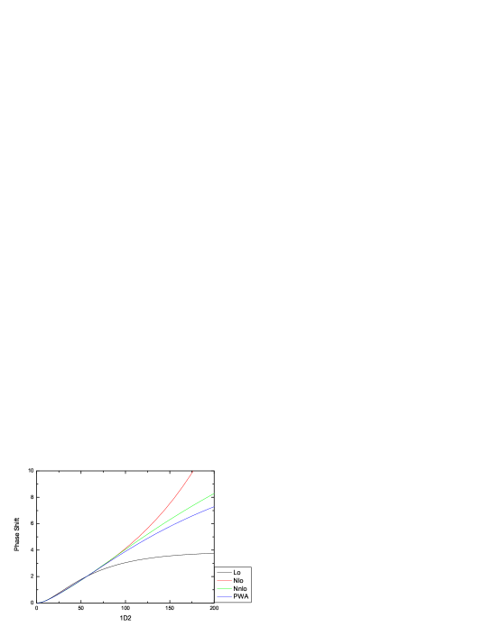
Here the coefficients $g_{l;n}$ will inevitably be R/R dependent and must be determined together with the parameters in the potential from physical boundary conditions, say the empirical phase shifts in the low energy ends[20]. Investigations along this line are in progress[23] and the primary the results are interesting. In fact, there is several virtues in such analysis: Firstly, one needs not to carry out the concrete the renormalization of ${\mathcal{G}}$; Secondly, by comparing with low energy region of the empirical data of $NN$ scattering (say, $E\leq 50\texttt{Mev}$) one could in principle easily obtain the optimal values for the semi-phenomenological parameters ($g_{l;n}$) which in turn could yield a pretty good prediction of higher energy behaviors though the parametrization formula of Eq.( 3) is strikingly simple; Thirdly, with such simple tools one could test whether EFT systematically works for $NN$ scattering; Fourthly, one could also use it to estimate if the potential constructed up to a certain order is sufficient for various purposes without any loop calculations and renormalization operations. Moreover, due to its simplicity in principle, one might also find other uses like the estimation of the coupling constants of the local terms in constructed potential. This list could be further enlarged. We will visit them in the near future. In Fig. 1 we serve a primary example for such analysis[23] employing the potential given by EGM[4]: the phase shifts of ${}^{1}D_{2}$ channel predicted only with a single parameter $Re({\mathcal{G}}_{l=2})\approx g_{l=2;0}$ with potentials input at leading order (Lo), next-to-leading order (Nlo) and next-to-next-to-leading order (Nnlo), respectively. It is clear that the prediction of the phase shift for the range $50\texttt{Mev}\leq E\leq 200\texttt{Mev}$ with only one optimized or fitted parameter of $Re({\mathcal{G}}_{l=2})$, $g_{l=2;0}$, improves with the chiral order for the constructed potential (Lo, Nlo, and Nnlo). For most channels this seems true. Of course, there could well be exceptions, which we interpret it as insufficiency of the chiral expansion in the corresponding channel(s).

In summary, we proposed a simple and novel parametrization for understanding the nonperturbative renormalization of the $T$-matrix for nucleon-nucleon scattering. The distinctive feature of the nonperturbative renormalization–the failure of ’exogenous’ counter terms or the need of ’endogenous’ ones–is clarified together with some related issues like consistency of W power counting. By the way we could derive other uses from our simple parametrization of the $T$-matrix that might be of some academic values. We hope our investigation might be useful for a number of important issues related to nucleon interactions, and also to other nonperturbative problems.

Figure 1: The prediction of the phase shifts versus energy $E$ (Mev) of ${}^{1}D_{2}$ channel at LO, Nlo and Nnlo with the simplest parametrization $Re({\mathcal{G}}_{l=2})=g_{l=2;0}$. Also listed is the curve for PWA. For each order the $g_{2;0}$ is fitted to or optimized in the low energy region of the PWA data.

References

- [1] S. Weinberg, Phys. Lett. B 251, 288 (1990); Nucl. Phys. B 363, 1 (1991).
- [2] See, e.g., P. Bedaque and U. van Kolck, Ann. Rev. Nucl. Part. Sci. 52, 339 (2002).
- [3] C. Ordóñez, L. Ray and U. van Kolck, Phys. Rev. C53, 2086 (1996); U. van Kolck, Nucl. Phys. A645, 327 (1999).
- [4] E. Epelbaum, W. Glöckle and U. Meissner, Nucl. Phys. A637, 107 (1998), Nucl. Phys. A671, 295 (2000), Eur. Phys. J. A15, 543 (2002), arXiv:nucl-th/0304037, 0308010.
- [5] D.R. Phillips, S.R. Beane and T.D. Cohen, Ann. Phys.(NY) 263, 255(1998) and references therein.
- [6] J.V. Steele and R.J. Furnstahl, Nucl. Phys. A637, 46 (1999); T.S. Park, K. Kubodera, D.P. Min and M. Rho, Phys. Rev. C58, 637 (1998); T. Frederico, V.S. Timóteo and L. Tomio, Nucl. Phys. A653, 209 (1999).
- [7] D.B. Kaplan, M.J. Savage and M.B. Wise, Phys. Lett. B424, 390 (1998); Nucl. Phys. B534, 329 (1998); S. Fleming, T. Mehen and I.W. Stewart, Nucl. Phys. A677, 313 (2000); Phys. Rev. C61, 044005 (2000).
- [8] J. Gegelia, Phys. Lett. B463, 133 (1999); J. Gegelia and G. Japaridze, Phys. Lett. B517, 476 (2001); J. Gegelia and S. Scherer, arXiv:nucl-th/0403052.
- [9] D. Eiras and J. Soto, Eur. Phys. J. A17, 89 (2003).
- [10] S.R. Beane, P. Bedaque, M.J. Savage and U. van Kolck, Nucl. Phys. A700, 377 (2002).
- [11] J.A. Oller, arXiv:nucl-th/0207086.
- [12] D.B. Kaplan, Nucl. Phys. B494, 471 (1997); J. Nieves, Phys. Lett. B568, 109 (2003).
- [13] M. Pavon Valderrama and E. Ruiz Arriola, Phys, Lett. B580, 149 (2004), arXiv:nucl-th/0405057.
- [14] C.P. Burgess and D. London, Phys. Rev. D48, 4337 (1993).
- [15] For examples in other contexts, see, e.g., J.-F. Yang and J.-H. Ruan, Phys. Rev. D65, 125009 (2002) and references therein.
- [16] P.M. Stevenson, Phys. Rev. D23, 2916 (1981); G. Grunberg, Phys. Rev. D29, 2315 (1984); S.J. Brodsky, G.P. Lepage and P.B. Mackenzie, Phys. Rev. D28, 228 (1983).
- [17] S. Weinberg, Physica A96, 327 (1979); J. Gasser and H. Leutwyler, Ann. Phys. 158, 142 (1984); J. Gasser and H. Leutwyler, Nucl. Phys. B250, 465 (1985).
- [18] R.G. Newton, Scattering Theory of Waves and Particles, 2nd Edition (Springer-Verlag, New York, 1982), p187.
- [19] R. Jackiw, in M.A.B. Bég Memorial Volume, A. Ali and P. Hoodbhoy, eds. ( World Scientific, Singapore, 1991), p25-42.
- [20] V.G.J. Stoks, R.A.M. Klomp, M.C.M. Rentmeester, and J.J. de Swart, Phys. Rev. C48, 792 (1993).
- [21] Ji-Feng Yang, arXiv: hep-th/9708104; invited talk in: Proceedings of the XIth International Conference ’Problems of Quantum Field Theory’98’, Eds. B. M. Barbashov et al, (Publishing Department of JINR, Dubna, 1999), p.202[arXiv:hep-th/9901138]; arXiv: hep-th/9904055.
- [22] See the recent debates on the chiral limit nuclear forces: S.R. Beane and M.J. Savage, Nucl. Phys. A713, 148 (2003); Nucl. Phys. A717, 91 (2003); E. Epelbaum, W. Glöckle and U.-G. Meissner, Nucl. Phys. A714, 535 (2003).
- [23] J.-F. Yang and Jian-Hua Huang, in preparation.