Damped collective motion of many body systems:
A variational approach to the quantal decay rate

Abstract

We address the problem of collective motion across a barrier like encountered in fission. A formula for the quantal decay rate is derived which bases on a recently developed variational approach for functional integrals. This formula can be applied to low temperatures that have not been accessible within the former PSPA type approach. To account for damping of collective motion one particle Green functions are dressed with appropriate self-energies.

1 Introduction

For a particle moving in a metastable potential J.S. Langer [1] has shown that the decay rate

$$R=\frac{|\kappa|}{\pi T}\ \textrm{Im}\,\mathcal{F}$$ (1)

can be calculated from the partition function $\mathcal{Z}$ via the imaginary part of the free energy

$$\mathcal{F}=-T\ \textrm{ln}\,\mathcal{Z}\,.$$ (2)

(As usual temperature is measured in MeV such that the Boltzmann constant is put equal to $k_{\textrm{B}}\equiv 1$.) The parameter $1/\kappa$ (where $\kappa<0$) sets the time scale for the solution $\langle q\rangle_{t}=\langle q\rangle_{t=0}\ \exp(-\kappa t)$ which describes the motion of the average trajectory away from the barrier top. Using path integrals Langer’s formula has extensively been exploited in the framework of the Caldeira-Leggett model (CLM) [2] for dissipative quantum systems. Within this model the decay rate has been studied in great detail from high to very low temperatures. The region of the “crossover temperature” $T_{0}$, below which quantum tunneling becomes more important than pure thermal activation has been treated in [3, 4, 5]; for reviews on this subject see e.g. [6, 7].

In the present paper we want to adapt similar methods to systems like finite nuclei, where the dynamics of the particles is governed by a varying mean field. Different to the CLM this field, and hence the ”heat bath”, changes with the variable which parameterizes the path along which the free energy exhibits the barrier. A first attempt along these lines was reported in [8]. There, the partition function was calculated by accounting for correlations around the mean trajectory which were of RPA-type. In different context such an approach to $\mathcal{Z}$ has been phrased ”Perturbed Static Path Approximation” (PSPA), for details see [9, 10, 11]. As this method is based on a quadratic expansion of the effective action about stationary points it suffers the same breakdown as an analogous expansion within the CLM; the rate diverges at the $T_{0}$. In the present paper we like to overcome this problem by employing a variational approach to the quantum partition function, suggested recently in [12, 13].

At finite temperature nuclear collective motion is damped. In [8] this feature was simulated by applying simple energy smearing to the results obtained within the independent particle model (IPM). In the present paper we like to apply a more microscopic picture. The latter bases on the replacement of the one-body Green function of the IPM by dressed ones, accounting in this way for incoherent scattering processes among the particles. In this way connection is established to transport theory for damped collective motion (see e.g. [14, 15]). Indeed, by using linear response functions we are able to introduce microscopically transport coefficients like the inertia $M$, friction $\gamma$ or the stiffness $C$, which then may serve as input for the calculation of the decay rate of metastable systems.

The paper is organized as follows: In Sect. 2 we briefly review several approximations to the partition function $\mathcal{Z}$ of interacting many body systems. Thereafter in Sect. 3 we take into account residual interactions, apply linear response theory to treat damped harmonic motion and establish the connection to microscopic transport theories. In Sect. 4 we modify the methods of Sect. 2 such that dissipation can be treated. After the derivation of formulas for the decay rate of metastable interacting many body systems in Sect. 5 we want to estimate the accuracy of our results. In the ideal case this should be done with an exactly solvable model for the many body system. However, to the best of our knowledge for damped collective motion, the case we are interested in, such a model does not exist. For this reason so far we are only able to test in Sect. 6 our approach at the example of a particle moving in a one-dimensional potential under the influence of damping, leaving a more involved analysis for many body systems for future work. Finally we like to close by discussing our findings and drawing some conclusions.

2 Approximations to the partition function

The collective degree of freedom shall be introduced through a mean field approximation to a separable interaction of the type [16] $k\hat{F}^{2}/2$. It is to be added to the unperturbed Hamiltonian $\hat{H}$, which at first shall be assumed to be of one body nature. The total $\hat{\cal H}$ thus is given by

$$\hat{\cal H}=\hat{H}+\frac{k}{2}\,\hat{F}\hat{F}\,.$$ (3)

For $k<0$ the interaction is attractive and leads to iso-scalar modes in the nuclear case. The operator $\hat{F}$ is meant to represent an effective generator of collective motion along a fission path. For the evaluation of the partition function $\mathcal{Z}$ we want to exploit functional integrals in imaginary time $\tau=0\ldots\hbar\beta$ with $\beta=1/T$. The two body interaction may then be treated by the Hubbard-Stratonovich transformation (HST) to the mean field Hamiltonian

$$\hat{\mathcal{H}}_{\textrm{HST}}[q(\tau)]=\hat{H}+q(\tau)\,\hat{F}\,.$$ (4)

Here, the $q(\tau)$ represents the collective variable. Following [17] it will be treated by an expansion around an average value $q_{0}$ defined through $\hbar\beta q_{0}=\int_{0}^{\hbar\beta}d\tau\,q(\tau)$. The deviation will be expanded into the Fourier series $q(\tau)-q_{0}=\sum_{r\neq 0}q_{r}\exp(\textrm{i}\nu_{r}\tau)$, with the Matsubara frequencies $\nu_{r}=(2\pi/\hbar\beta)\,r$ and $q_{-r}=q_{r}^{*}$. As described elsewhere (see e.g. [10, 18, 13]) the partition function can be expressed by the following (ordinary) integral over the $q_{0}$:

$$\mathcal{Z}(\beta)=\sqrt{\frac{\beta}{2\pi|k|}}\int_{-\infty}^{+\infty}\!\!dq_{0}\ \exp(-\beta\mathcal{F}^{\textrm{SPA}}(\beta,q_{0}))\ \zeta(\beta,q_{0})$$ (5)

In this expression $\mathcal{F}^{\textrm{SPA}}$ is the $q_{0}$-dependent effective free energy in the quasi-static picture, left over here in the classical limit, where all $\tau$-dependent deviations from $q_{0}$ can be neglected. For convenience we introduce the effective free energy

$$\mathcal{F}^{\textrm{eff}}(\beta,q_{0})=\mathcal{F}^{\textrm{SPA}}(\beta,q_{0})-\frac{1}{\beta}\ \textrm{ln}\,\zeta(\beta,q_{0})\,,$$ (6)

which includes quantum effects through the factor $\zeta$. This correction still is a functional integral in $q_{r}$-space and specified through an Euclidean action $s_{\textrm{E}}(\beta,q_{0})$. Various existing approximations consist in the way this action is treated. As already indicated through the notation employed in (5) and (6), within the Static Path Approximation (SPA) the $\zeta^{\textrm{SPA}}$ is put equal to unity, which implies to discard all fluctuations around $q_{0}$. Corrections to this approximation (see e.g. [13]) are obtained by expanding systematically the action

$$s_{\textrm{E}}=\frac{\hbar\beta}{|k|}\left(\sum_{r,s\neq 0}\lambda_{rs}\,q_{r}q_{s}+\sum_{r,s,t\neq 0}\rho_{rst}\,q_{r}q_{s}q_{t}+\sum_{r,s,t,u\neq 0}\sigma_{rstu}\,q_{r}q_{s}q_{t}q_{u}\right)+{\cal O}(q_{r}^{5})$$ (7)

around the static path $q_{0}$ to some power in the $q_{r}$, exhibited here to fourth order.

Within the SPA+RPA [9], the Perturbed Static Path Approximation (PSPA) [10] or the Correlated Static Path Approximation (CSPA) [11] the expansion (7) is truncated after the second order

$$s_{\textrm{E}}^{\textrm{PSPA}}=\frac{\hbar\beta}{|k|}\sum_{r,s\neq 0}\lambda_{rs}\,q_{r}q_{s}\,.$$ (8)

This approximation takes into account quantum fluctuations around $q_{0}$ on the level of local RPA modes. It turns out (see e.g. [8]) that the second order coefficients of the PSPA are diagonal $\lambda_{rs}=\lambda_{r}/2\ \delta_{r,-s}$, with the $\lambda_{r}$ being given by

$$\lambda_{r}(\beta,q_{0})=1+k\,\chi(\textrm{i}\nu_{r})=\frac{\prod_{\mu}(\nu_{r}^{2}+\varpi_{\mu}^{2}(\beta,q_{0}))}{\prod_{k>l}^{\prime}(\nu_{r}^{2}+\omega_{kl}^{2}(q_{0}))}\,.$$ (9)

Here, the response function $\chi(\omega)$ has been introduced, which is defined through the relation

$$\delta\langle\hat{F}\rangle_{\omega}=-\chi(\omega)\,\delta q(\omega)$$ (10)

where $\delta q(\omega)$ means a general time-dependent deviation from $q_{0}$. Mind that the averages have to be calculated from the Hamiltonian (4) at fixed $q_{0}$. In this way the $\chi(\omega)$ depends on $\beta$ and $q_{0}$. Since this $\chi(\omega)$ only contains excitations of nucleonic nature,

$$\hbar\omega_{kl}=\epsilon_{k}-\epsilon_{l}\,,$$ (11)

which are to be distinguished from collective ones (to which we will come to below), we may call it the nucleonic or intrinsic response function. In the following the single particle energies shall be measured with respect to the chemical potential $\mu$, which means to write $\hbar\omega_{k}(q_{0})=\epsilon_{k}(q_{0})-\mu(q_{0})$. The local RPA frequencies $\varpi_{\mu}(\beta,q_{0})$ appearing in (9) must be calculated from the secular equation

$$1+k\chi(\varpi_{\mu})=0\,.$$ (12)

Note that the important factors in the product (9) are those which deviate from one. This happens whenever the $\varpi_{\mu}^{2}$ is sizably different from the corresponding $\omega_{kl}^{2}$. This is so in particular for the typical collective modes, for which for stable isoscalar modes, for instance, one has $\varpi_{\mu}^{2}\ll\omega_{kl}^{2}$.

For proper convergence of the path integral for $\zeta^{\textrm{PSPA}}$ one needs the condition (see e.g. [18, 13])

$$\lambda_{1}(\beta,q_{0})>0\,.$$ (13)

It ensures the PSPA to be well defined such that the quantum corrections can be written in the form

$$\zeta^{\textrm{PSPA}}(\beta,q_{0})=\prod_{r>0}\frac{1}{\lambda_{r}(\beta,q_{0})}\,.$$ (14)

The restriction (13) can easily be translated into a condition on that temperature at which an unphysical divergence of the quantum fluctuations around $q_{0}$ occurs: $T>T_{0}$. Here

$$T_{0}=\textrm{Max}_{q_{0}}\,\frac{\hbar|\varpi_{\textrm{inst}}(q_{0})|}{2\pi}$$ (15)

can be calculated from the unstable local RPA mode for which $\varpi_{\textrm{inst}}^{2}<0$. The latter is present whenever $\mathcal{F}^{\textrm{SPA}}(q_{0})$ develops a barrier.

Obviously, the unphysical divergence at $T_{0}$ is a deficiency of the PSPA. It can be cured by accounting for inharmonicities in the expansion (7) of the action. To be able to lower the breakdown temperature to $T_{0}/2$ it is sufficient to concentrate on the three coefficients $\rho_{1,1,-2}$, $\rho_{-1,-1,2}$ and $\sigma_{1,1,-1,-1}$ and neglect the remaining ones [18]. This improved approximation was called extended Perturbed Static Path Approximation (ePSPA). For $T>T_{0}/2$ the quantum correction factor may then be expressed by the form

$$\zeta^{\textrm{ePSPA}}(\beta,q_{0})=\sqrt{\pi}\ \frac{x(\beta,q_{0})}{\lambda_{1}(\beta,q_{0})}\ \exp\left[x^{2}(\beta,q_{0})\right]\,\textrm{erfc}\left[x(\beta,q_{0})\right]\ \prod_{r>1}\frac{1}{\lambda_{r}(\beta,q_{0})}\,.$$ (16)

The quantity

$$x=\sqrt{\frac{\beta}{4|k|B}}\ \lambda_{1}\qquad\textrm{with}\qquad B=6\sigma_{1,1,-1,-1}-\frac{9\rho_{-1,-1,2}\rho_{1,1,-2}}{\lambda_{2}}$$ (17)

is given in terms of the third and fourth order inharmonic terms of the Euclidean action (7). The coefficients $\rho$ and $\sigma$ can be expressed through one body Green’s functions

$$g_{k}^{(0)}(z)=\frac{1}{\hbar}\,\frac{1}{z-\omega_{k}}$$ (18)

corresponding to the static part of the Hamiltonian (4). Details of the calculation can be found in [18, 12]. With Fermi occupation numbers denoted by $n(\epsilon_{k})$ the general coefficient $\sigma_{rstu}$ consists of a sum of terms like

$$\frac{|k|}{4!}\sum_{i,k,m,o}F_{io}F_{ki}F_{mk}F_{om}\times$$ (19)

$$\left\{n(\epsilon_{i})\ g_{o}^{(0)}(\omega_{i}+\textrm{i}\nu_{r})\ g_{k}^{(0)}(\omega_{i}-\textrm{i}\nu_{s})\ g_{m}^{(0)}(\omega_{i}-\textrm{i}\nu_{s+t})\right.$$

$$+\ n(\epsilon_{o})\ g_{i}^{(0)}(\omega_{o}-\textrm{i}\nu_{r})\ g_{k}^{(0)}(\omega_{o}-\textrm{i}\nu_{r+s})\ g_{m}^{(0)}(\omega_{o}-\textrm{i}\nu_{r+s+t})$$

$$+\ n(\epsilon_{k})\ g_{i}^{(0)}(\omega_{k}+\textrm{i}\nu_{s})\ g_{o}^{(0)}(\omega_{k}+\textrm{i}\nu_{r+s})\ g_{m}^{(0)}(\omega_{k}-\textrm{i}\nu_{t})$$

$$\left.+\ n(\epsilon_{m})\ g_{i}^{(0)}(\omega_{m}+\textrm{i}\nu_{s+t})\ g_{o}^{(0)}(\omega_{m}+\textrm{i}\nu_{r+s+t})\ g_{k}^{(0)}(\omega_{m}+\textrm{i}\nu_{t})\right\}\,.$$

The $\rho_{rst}$ or the higher order coefficients are of similar structure.

Recently for the many body system studied here, a variational approach to the quantum corrections $\zeta$ of (6) has been developed in [12, 13]. Based on the Euclidean action of the PSPA (8) a reference action

$$s_{\Omega}^{q_{0}}=\frac{\hbar\beta}{|k|}\sum_{r>0}\Lambda_{r}\,|q_{r}|^{2}\,.$$ (20)

is introduced, where the RPA frequencies $\varpi_{\mu}^{2}$ appearing in (9) are replaced by variational parameters $\Omega_{\mu}^{2}$:

$$\Lambda_{r}(\beta,q_{0};\Omega_{\mu})=\frac{\prod_{\mu}(\nu_{r}^{2}+\Omega_{\mu}^{2}(\beta,q_{0}))}{\prod_{k>l}^{\prime}(\nu_{r}^{2}+\omega_{kl}^{2}(q_{0}))}$$ (21)

The $\Omega_{\mu}^{2}$ are adjusted such that the expectation value $\langle s_{\textrm{E}}-s_{\Omega}^{q_{0}}\rangle_{\Omega}^{q_{0}}$ with respect to the $s_{\Omega}^{q_{0}}$ and consequently the effective free energy (6) is minimized. Accounting in the action (7) for inharmonic terms up to fourth order and using the abbreviation

$$\Pi_{r}(\beta,q_{0};\Omega_{\mu})=\frac{\prod_{\mu}(\nu_{r}^{2}+\varpi_{\mu}^{2})-\prod_{\mu}(\nu_{r}^{2}+\Omega_{\mu}^{2})}{\prod_{\mu}(\nu_{r}^{2}+\Omega_{\mu}^{2})}$$ (22)

within this approximation the correction factor of the variational approach can be written as [12, 13]

$$\textrm{ln}\,\zeta^{\textrm{(4)}}(\beta,q_{0})=-\sum_{r>0}\textrm{ln}\Lambda_{r}-\sum_{r>0}\Pi_{r}-\frac{|k|}{\beta}\sum_{r,s>0}\sigma_{rs-r-s}\,\frac{1}{\Lambda_{r}}\,\frac{1}{\Lambda_{s}}\,.$$ (23)

Here, the fourth order coefficient $\sigma_{rstu}$ again is calculated according to (19). For convergence of the double sum in the second line of (23) the behavior of $\sigma_{rstu}$ at large $r,s,\ldots$ is crucial. By inspection of (19), using the unperturbed Green’s functions (18) and $\nu_{r}\sim r$, one can convince one-self that $\sigma_{rstu}$ falls off rapidly enough to assure convergence.

This variational approach [12, 13] to the partition function of an interacting many body system improves the accuracy of the PSPA and the ePSPA. Moreover, even in cases where the static free energy $\mathcal{F}^{\textrm{SPA}}$ develops a barrier (as a function of $q_{0}$), this novel approach still is applicable below $T_{0}$ or $T_{0}/2$. Evidently, this variational approach is the easier to handle the fewer variational parameters $\Omega_{\mu}$ one needs to introduce. For the present formulation the latter are unequivocally related to the RPA frequencies $\varpi_{\mu}$ of the secular equation (12). In principle, the latter has as many solutions as there are p-h excitations. However, as already discussed below (9), not all of them are equally important for collective motion. In the ideal case the latter is dominated by only a few or eventually by just one prominent mode. Then it suffices to concentrate on these or this latter one(s) [13].

3 Accounting for residual interactions

So far the operator $\hat{H}$ appearing in (3) and (4) is identified with that of the independent particle model (IPM), with the corresponding excitations given by (11) and the one body Green’s functions by (18). The response function defined by (10) can be written in the form $\chi(\omega)=\chi^{\prime}(\omega)+\textrm{i}\chi^{\prime\prime}(\omega)$. Calculated from the IPM its imaginary part $\chi^{\prime\prime}$ consists of a sum of $\delta$-functions located at discrete energies. However, the IPM neglects the residual two body interaction between the nucleons, which describes the incoherent scattering of particles and holes and consequently couples the $1$p$1$h excitations of (4) to $n$p$n$h excitations and true compound states. It is this residual interaction which in the end is responsible for genuine relaxation processes and, hence, for damping of collective motion. To account for such effects we will take a pragmatic point of view. Rather than to embark on the difficult (if at all feasible) task to account for the residual interaction in full glory we will simply take over the factorization of the response function into one body Green’s functions $g_{k}(z)$, which using the corresponding spectral densities $\varrho_{k}(z)$ leads to

$$\chi(z)=-\hbar\sum_{l,k}F_{lk}F_{kl}\int_{-\infty}^{\infty}\frac{d\Omega}{2\pi}\ n(\hbar\Omega+\mu)\left[g_{k}(z+\Omega)\varrho_{l}(\Omega)+\varrho_{k}(\Omega)g_{l}(\Omega-z)\right]\,.$$ (24)

For a more detailed description we refer to [15] where also references to earlier work can be found. Different to the IPM we dress the Green’s functions by self-energies $\Sigma_{k}=\Sigma_{k}^{\prime}-\textrm{i}\Gamma_{k}/2$ and write

$$g_{k}^{(\Gamma)}(z)=\frac{1}{\hbar}\,\frac{1}{z-\omega_{k}-\Sigma_{k}(z)/\hbar}\,.$$ (25)

instead of (18). These self-energies are calculated from

$$\Sigma_{k}(z)=\int_{-\infty}^{\infty}\frac{d\Omega}{2\pi}\,\frac{\Gamma_{k}(\Omega)}{z-\Omega}$$ (26)

with the following phenomenological ansatz for the widths

$$\Gamma_{k}(\omega)=\frac{1}{\Gamma_{0}}\,\frac{(\hbar\omega-\mu)^{2}+\pi^{2}T^{2}}{1+\frac{1}{c^{2}}[(\hbar\omega-\mu)^{2}+\pi^{2}T^{2}]}\,.$$ (27)

As for the two parameters introduced this way, the values $\Gamma_{0}\approx 33~{}\textrm{MeV}$ and $c\approx 20~{}\textrm{MeV}$ have been used in the past (see e.g. [14] and [15]). It can be said that at zero temperature the widths calculated this way are in good agreement with empirical data for single particle excitations [19]. Moreover, at $T=0$ forms of this type have been used in [20] in analyses of experimental results within optical model type approaches, for more details see Sect. 4.2.3. of [15].

We should like to note that the factorization assumption leading to (24) is applied to describe the intrinsic dynamics but not that of collective modes. One may therefore argue that coherent effects are small, in particular at larger thermal excitations. After all the underlying SPA is meant to represent the high temperature limit.

We may proceed now to establish connection to microscopic transport theories like the one described in [15]. To this end it us useful to introduce the collective response function defined by

$$\delta\langle\hat{F}\rangle_{\omega}=-\chi_{\textrm{coll}}(\omega)\,f_{\textrm{ext}}(\omega)\,,$$ (28)

where $f_{\textrm{ext}}$ stands for an external field coupled to (4) via $f_{\textrm{ext}}(\tau)\hat{F}$. As is well known (see e.g. [16] or [15]) it can be obtained from the nucleonic response function of (10) through

$$\chi_{\textrm{coll}}(\omega)=\frac{\chi(\omega)}{1+k\,\chi(\omega)}$$ (29)

Its poles are given by the solutions of the secular equation (12). Very similar to the situation discussed in connection with (9), not all those poles $\varpi_{\mu}$ contribute equally strongly. In the ideal case one of them is shifted down to frequencies which are much smaller than the corresponding nucleonic excitations ($|\varpi_{\mu}|^{2}\ll\omega_{kl}^{2}$ for stable iso-scalar modes). Moreover, it may acquire a considerable part of the overall strength.

In order to take into account dissipative effects we perform two modifications. As mentioned previously, the nucleonic response function $\chi(\omega)$ is calculated from the dressed Green’s functions (25) instead of (18). Using the $\Gamma$ of (27) the imaginary part $(\chi^{\Gamma})^{\prime\prime}(\omega)$ becomes a continuous function of $\omega$. As we are interested in a description of slow iso-scalar collective motion, as given for instance for nuclear fission, we will concentrate on the lowest lying (pair of) poles of the (locally defined) collective response function (29). This truncated form is fitted by the response function of a damped harmonic oscillator of inertia $M$, stiffness $C$ and damping $\gamma$

$$\chi_{\textrm{osc}}(\omega)=\frac{-1}{M\omega^{2}+\textrm{i}\gamma\omega-C}=\frac{1}{|C|}\,\frac{-1}{(\omega/\varpi)^{2}+2\textrm{i}\eta\omega/\varpi-\textrm{sgn}C}\,.$$ (30)

Then, instead of several $\varpi_{\mu}$ only one collective mode $\varpi$ is left over. The frequency $\varpi$ and the effective damping coefficient $\eta$ are defined as follows:

$$\varpi^{2}=\frac{|C|}{M}\qquad\textrm{and}\qquad\eta=\frac{\gamma}{2M\varpi}=\frac{\gamma}{2\sqrt{M|C|}}$$ (31)

The parameter $\eta$ indicates underdamped ($\eta<1$) or overdamped motion ($\eta>1$). After these modifications, which may be summarized as

$$\chi_{\textrm{coll}}^{\textrm{IPM}}(\omega)\longrightarrow\chi_{\textrm{coll}}^{\Gamma}(\omega)\longrightarrow\chi_{\textrm{osc}}(\omega)\,,$$ (32)

the secular equation (12) for the local collective modes reduces to the equation

$$\left(\frac{\omega}{\varpi}\right)^{2}+2\textrm{i}\eta\left(\frac{\omega}{\varpi}\right)-\textrm{sgn}C=0\,.$$ (33)

Its solutions are given by the two frequencies

$$\omega_{\pm}=\varpi\left(\pm\sqrt{\textrm{sgn}C-\eta^{2}}-\textrm{i}\eta\right)\,.$$ (34)

In contrast to the RPA frequencies $\varpi_{\mu}$ of the IPM, the $\omega_{\pm}$ have a finite imaginary part. This implies a damped local collective motion due to the influence of the residual interaction.

At this place it is important to stress that the transport coefficients $C=C(T,q_{0})$, $\eta=\eta(T,q_{0})$ and $\varpi=\varpi(T,q_{0})$ or $M=M(T,q_{0})$ and $\gamma=\gamma(T,q_{0})$ have been derived from a microscopic quantum theory starting from the separable two body interaction (3). Like the response function itself, all of them depend on the temperature $T=1/\beta$ and the collective coordinate $q_{0}$. With respect to nuclear collective motion this dependence may be considered a great advantage over the Caldeira-Leggett model (CLM) [2], which is often used to describe open quantum systems (see e.g. [7]; for a criticism from nuclear physics point of view, see [15, 12]). There, the transport coefficients are not calculated microscopically. Rather they are introduced as parameters which are independent of $T$ and $q_{0}$. This latter feature goes along with the fact that in the CLM the set of intrinsic degrees of freedom, which acts as the “heat bath” for the collective ones, is modeled by a set of fixed harmonic oscillators. The latter do not vary with the collective degree of freedom, and so does the spectral density. Such an assumption is not applicable to nuclear fission. There the heat bath for collective motion is given by the nucleonic degrees of freedom which move in a mean field which depends on the nuclear shape and thus varies with the collective variable.

4 Dissipative systems: Modification of the approximations to the partition function

In this section we study how the inclusion of dissipative effects modifies the approximations put together in Sect. 2 in formal sense. First we look at the PSPA. After the reduction (32) to a single damped mode an evaluation of

$$\lambda_{r}=1+k\,\chi(\textrm{i}\nu_{r})=\frac{1}{1-k\,\chi_{\textrm{coll}}(\textrm{i}\nu_{r})}$$ (35)

(see (9) and (29)) leads to

$$\lambda_{r}\to\lambda_{r}^{(\Gamma)}=\frac{\nu_{r}^{2}+\nu_{r}/\tau_{\textrm{kin}}+\textrm{sgn}C\,\varpi^{2}}{\nu_{r}^{2}+\nu_{r}/\tau_{\textrm{kin}}+w^{2}}\,.$$ (36)

Here, the (inverse) time scale

$$\frac{1}{\tau_{\textrm{kin}}}=\frac{\gamma}{M}$$ (37)

and the quantity

$$w^{2}(\beta,q_{0})=\frac{C-k}{M}=\textrm{sgn}C\,\varpi^{2}(\beta,q_{0})+\frac{|k|}{M(\beta,q_{0})}\geq\textrm{sgn}C\,\varpi^{2}(\beta,q_{0})$$ (38)

have been introduced. A calculation of the nucleonic response function

$$\chi(\omega)=\frac{-1}{M\omega^{2}+\textrm{i}\gamma\omega-(C-k)}$$ (39)

from (30) by inversion of the formula (29) shows that $w^{2}$ plays the role of the nucleonic frequencies. In dissipative PSPA the form of the quantum corrections to the classical partition function defined in (5) does not change as compared to the IPM (14). Only the $\lambda_{r}$ are replaced by the $\lambda_{r}^{(\Gamma)}$ of (36). The convergence condition (13) now turns to $\lambda_{1}^{(\Gamma)}(\beta,q_{0})>0$ and explicitly reads

$$\left(\frac{2\pi}{\hbar\beta}\right)^{2}+\frac{1}{\tau_{\textrm{kin}}}\,\frac{2\pi}{\hbar\beta}+\textrm{sgn}C\,\varpi^{2}>0$$ (40)

In the case of stable modes with $C>0$ this condition is always fulfilled. For unstable modes with $C<0$, in analogy to (15) the local crossover temperature $T_{0}(q_{0})$ is given by the smallest root of the l.h.s. of the inequality (40). Using the effective damping $\eta$ of (31) this $T_{0}(q_{0})$ becomes

$$T_{0}(q_{0})=\frac{\hbar\varpi(q_{0})}{2\pi}\left(\sqrt{1+\eta^{2}(q_{0})}-\eta(q_{0})\right)\,.$$ (41)

Its maximal value $T_{0}=\textrm{Max}_{q_{0}}T_{0}(q_{0})$ defines the global crossover temperature. Like in the CLM for dissipative quantum systems (see e.g. [5, 6, 7]) we find that damping $\eta>0$ diminishes this $T_{0}$.

Concerning the anharmonic terms of the Euclidean action there is an important difference between our approach and the CLM. In the latter the conservative and the dissipative forces are decoupled from each other. As one implication, for instance, the inharmonic terms of the potential $V^{(n)}(q)$ with $n>2$ are not modified by dissipative effects. In the case of interacting many body systems the situation is more complicated: The replacement of the unperturbed Green’s functions (18) by the dressed ones (25) not only leads to a finite damping strength $\eta$ and a change in the frequency of the local harmonic motion $\omega_{\pm}$. Due to the structure (19) of the expansion coefficients of the Euclidean action (7) also the inharmonic terms are influenced by this replacement, such that $\rho_{rst}\to\rho_{rst}^{(\Gamma)}$ and $\sigma_{rstu}\to\sigma_{rstu}^{(\Gamma)}$. Taking into account dissipative effects for the quantum corrections of the ePSPA along the lines of [18] one can easily rederive (16), but with $\lambda_{r}\to\lambda_{r}^{(\Gamma)}$ and

$$x\to x^{(\Gamma)}=\sqrt{\frac{\beta}{4|k|B^{(\Gamma)}}}\ \lambda_{1}^{(\Gamma)}\,,$$ (42)

where

$$B^{(\Gamma)}=6\sigma_{1,1,-1,-1}^{(\Gamma)}-\frac{9\rho_{-1,-1,2}^{(\Gamma)}\,\rho_{1,1,-2}^{(\Gamma)}}{\lambda_{2}^{(\Gamma)}}\,.$$ (43)

Using the variational approach in order to account for dissipative features the form

$$s_{\Omega}^{q_{0}}=\frac{\hbar\beta}{|k|}\sum_{r>0}\Lambda_{r}^{(\Gamma)}\,|q_{r}|^{2}$$ (44)

with

$$\Lambda_{r}^{(\Gamma)}(\beta,q_{0};\Omega)=\frac{\nu_{r}^{2}+\nu_{r}/\tau_{\textrm{kin}}+\Omega^{2}}{\nu_{r}^{2}+\nu_{r}/\tau_{\textrm{kin}}+w^{2}}$$ (45)

is used as reference action. The trial action (44) contains only one variational parameter $\Omega^{2}$ and, analogously to the case sketched in Sect. 2, emerges from the dissipative version of $s_{\textrm{E}}^{\textrm{PSPA}}$ (see (8) with $\lambda_{r}^{(\Gamma)}$ of (36) instead of $\lambda_{r}$) by the replacement $\textrm{sgn}C\,\varpi^{2}\to\Omega^{2}$. Using (44) and repeating the derivation of [13] for the dissipative case the quantum correction factor to the classical partition function in the variational approach turns out to be given by (23) with the replacements $\Lambda_{r}\to\Lambda_{r}^{(\Gamma)}$,

$$\Pi_{r}\quad\rightarrow\quad\Pi_{r}^{(\Gamma)}(\beta,q_{0};\Omega)=\frac{\textrm{sgn}C\,\varpi^{2}-\Omega^{2}}{\nu_{r}^{2}+\nu_{r}/\tau_{\textrm{kin}}+\Omega^{2}}$$ (46)

and $\sigma_{rstu}\to\sigma_{rstu}^{(\Gamma)}$ everywhere:

$$\textrm{ln}\,\zeta^{\textrm{(4)}}(\beta,q_{0})=-\sum_{r>0}\textrm{ln}\Lambda_{r}^{(\Gamma)}-\sum_{r>0}\Pi_{r}^{(\Gamma)}-\frac{|k|}{\beta}\sum_{r,s>0}\sigma_{rs-r-s}^{(\Gamma)}\,\frac{1}{\Lambda_{r}^{(\Gamma)}}\,\frac{1}{\Lambda_{s}^{(\Gamma)}}$$ (47)

Please note that this form is very similar to that of the extension of the Feynman-Kleinert variational approach (FKV) [21] to open quantum systems (see e.g. [7]). There the quantum partition function of a particle of mass $M$ in a one-dimensional potential $V(q)$ and an oscillator heat bath environment has been studied within the CLM. Using the (inverse) time scale (37) and the fluctuation width [7]

$$a^{2}(\beta,q_{0})=\frac{2}{M\beta}\sum_{r>0}\frac{1}{\nu_{r}^{2}+\nu_{r}/\tau_{\textrm{kin}}(\nu_{r})+\Omega^{2}(\beta,q_{0})}$$ (48)

to fourth order in $a$ the quantum corrections read [7]:

$$\textrm{ln}\,\zeta^{\textrm{FKV}}(\beta,q_{0}) = \sum_{r>0}\textrm{ln}\,\frac{\nu_{r}^{2}}{\nu_{r}^{2}+\nu_{r}/\tau_{\textrm{kin}}(\nu_{r})+\Omega^{2}(\beta,q_{0})}$$

$$-\frac{\beta M}{2}\,[V^{\prime\prime}(q_{0})/M-\Omega^{2}(\beta,q_{0})]\,a^{2}(\beta,q_{0})$$

$$-\frac{\beta}{8}\,V^{(4)}(q_{0})\,(a^{2}(\beta,q_{0}))^{2}+\mathcal{O}(a^{6})$$

Recalling the definitions of $\Lambda_{r}^{(\Gamma)}$ and $\Pi_{r}^{(\Gamma)}$ in (45) and (46) respectively, the terms of (47) and (4) correspond to each other in the order of their appearence. In (47) the analog of the squared width (48) is a sum consisting of terms of the form $1/\Lambda_{r}^{(\Gamma)}$ (see (45)), which converge to $1$ in the limit $r\to\infty$. As mentioned already before, different to the fourth order term in (4) for convergence of the double sum in the last line of (47) the behavior of $\sigma_{rs-r-s}^{(\Gamma)}$ for large $r$ and $s$ is crucial. This difference can finally be traced back to the different path integral measures in both cases.

5 Decay of metastable states

In [8] a formula for the decay rate of damped interacting many body systems has been derived within the PSPA. Like that whole formalism it is applicable for $\beta<\beta_{0}$ only. For $\beta\to\beta_{0}$ the quantum corrections to the classical rate show an unphysical divergence. From the fact that the variational approach to the partition function can be applied also for $\beta>\beta_{0}$ we expect that a rate formula can be derived, which behaves well in the crossover region and beyond.

Based on Langer’s findings [1] for the decay rate $R$ of a metastable system in the literature (see e.g. [6] or [7]) for high temperatures the formula

$$R(\beta<\beta_{0})=-\frac{2}{\hbar}\ \frac{\beta}{\beta_{0}}\ \textrm{Im}\,{\mathcal{F}}(\beta)\,,$$ (50)

is in wide use. With the identifications $1/\beta_{0}=T_{0}$ (form (41) evaluated at the barrier $q_{0}=q_{b}$) and $|\kappa|=-\textrm{i}\omega_{+}$ (from (34) with $\varpi=\varpi_{b}$ and $\textrm{sgn}C=-1$) it becomes identical to (1). For the low temperature region I. Affleck has shown [22] that

$$R(\beta>\beta_{0})=-\frac{2}{\hbar}\ \textrm{Im}\,{\mathcal{F}}(\beta)$$ (51)

gives the same result as a Boltzmann average over the energy dependent decay rate $R=-2/\hbar\ \textrm{Im}\,E$. Of course, the formulas (50) and (51) coincide at $\beta=\beta_{0}$.

In the following we apply (50) and (51) to our modeling of interacting many body systems by the Hamiltonian (3). To this end the integral (5) for the partition function and its relation to the free energy of the total system (2) is used. This integral is dominated by the free energy $\mathcal{F}^{\textrm{SPA}}(q_{0})$ of the SPA. In the sequel the latter will be assumed to have just one minimum at $q=q_{a}$ and one barrier at $q=q_{b}$. (Whenever suitable the indices $a$ and $b$ will be used for quantities which have to be evaluated at the minimum and the barrier, respectively.) Moreover, we want to concentrate on examples where the barrier is sufficiently pronounced. First of all this implies that the (temperature-dependent) height $B^{\textrm{SPA}}=\mathcal{F}_{b}^{\textrm{SPA}}-\mathcal{F}_{a}^{\textrm{SPA}}$ is sufficiently large, as compared to temperature, $\beta B^{\textrm{SPA}}(\beta)\gg 1$. The minimum and the barrier are assumed to be well separated in $q_{0}$. In addition we assume that locally they may be approximated by oscillators with stiffnesses $C^{\textrm{SPA}}=\partial^{2}\mathcal{F}^{\textrm{SPA}}/\partial q_{0}^{2}$, with a positive $C^{\textrm{SPA}}_{a}$ and a negative $C^{\textrm{SPA}}_{b}$. Any further structure of $\mathcal{F}^{\textrm{SPA}}$ is neglected. Moreover, the variation of the quantum corrections $\textrm{ln}\,\zeta(\beta,q_{0})$ with $q_{0}$ should be sufficiently weak such that the integral (5) can be evaluated by a steepest descent approximation. The partition function

$$\mathcal{Z}(\beta)\approx\mathcal{Z}_{a}(\beta)+\textrm{i}\mathcal{Z}_{b}(\beta)$$ (52)

then develops an imaginary part which is associated to the stationary point at the saddle and given by

$$\mathcal{Z}_{b}(\beta)=\frac{1/2}{\sqrt{|k\,C_{b}^{\textrm{SPA}}(\beta)|}}\ \exp[-\beta\mathcal{F}_{b}^{\textrm{SPA}}(\beta)]\ \zeta_{b}(\beta)\,.$$ (53)

The real part

$$\mathcal{Z}_{a}(\beta)=\frac{1}{\sqrt{|k|\,C_{a}^{\textrm{SPA}}(\beta)}}\ \exp[-\beta\mathcal{F}_{a}^{\textrm{SPA}}(\beta)]\ \zeta_{a}(\beta)$$ (54)

comes from the stationary point at the minimum. To obtain (53) a special treatment is necessary for the integration around the barrier top. Following Langer [1], there the contour of integration must be distorted into the upper complex half plane. Because of the assumptions about the barrier height we have $\textrm{Im}\mathcal{Z}(\beta)\ll\textrm{Re}\mathcal{Z}(\beta)$, implying that the imaginary part of the free energy can be approximated by

$$\textrm{Im}\mathcal{F}(\beta)\approx-1/\beta\cdot\textrm{Im}\mathcal{Z}(\beta)/\textrm{Re}\mathcal{Z}(\beta)\,.$$ (55)

Using (50) or (51) the rate can be separated into a product of two factors, one representing the classical limit and the other the quantum corrections:

$$R(\beta)=R_{\textrm{class}}(\beta)\cdot f_{\textrm{qm}}(\beta)$$ (56)

Inserting the crossover temperature $T_{0}=1/\beta_{0}$ of (41) and the imaginary part of the free energy (55) into (50), for high temperatures the classical part reads:

$$R_{\textrm{class}}^{\textrm{SPA}}(\beta<\beta_{0})=\frac{\varpi_{b}(\beta)}{2\pi}\left(\sqrt{1+\eta_{b}^{2}(\beta)}-\eta_{b}(\beta)\right)\sqrt{\frac{C_{a}^{\textrm{SPA}}(\beta)}{C_{b}^{\textrm{SPA}}(\beta)}}\,\exp[-\beta B^{\textrm{SPA}}(\beta)]$$ (57)

This result has already been found in [8]. There it also had been rewritten in a more intuitive way by making use of (31) for the stiffnesses:

$$\frac{\varpi_{b}}{2\pi}\,\sqrt{\frac{C_{a}^{\textrm{SPA}}}{C_{b}^{\textrm{SPA}}}}=\frac{\varpi_{a}}{2\pi}\,\sqrt{\frac{M_{a}}{M_{b}}}$$ (58)

In this way in (57) besides the Arrhenius factor $\exp[-\beta B^{\textrm{SPA}}]$ the attempt frequency $\varpi_{a}$ appears, with which the system tries to overcome the barrier. Notice please that in this rate formula the factor in brackets is equivalent to Kramers’ famous correction factor [23]. It indicates that the classical contribution to the rate is reduced by damping. Different to the rate formulas derived in the CLM in (58) the ratio of the inertias at the barrier and the minimum appears [8]. It should be mentioned, however, that this additional factor is not seen in Langer’s original work although his derivation started from a Fokker-Planck equation where the inertia is allowed to depend on the collective variable. To clarify this point one may eventually have to modify the way the collective degree of freedom is introduced in the common SPA and PSPA formulations of the HST on which also our approach bases heavily.

For low temperatures application of (51) leads to

$$R_{\textrm{class}}^{\textrm{SPA}}(\beta>\beta_{0})=\frac{1}{\hbar\beta}\,\sqrt{\frac{C_{a}^{\textrm{SPA}}(\beta)}{C_{b}^{\textrm{SPA}}(\beta)}}\,\exp[-\beta B^{\textrm{SPA}}(\beta)]\,.$$ (59)

Note that this region has not been accessible with the PSPA in [8]. The formulas (57) and (59) describe the contribution of thermal activation to the decay rate.

Finally, we turn to the quantum correction factor $f_{\textrm{qm}}(\beta)$. Both for (57) as well as for (59) it has the same form,

$$f_{\textrm{qm}}(\beta)=\frac{\zeta_{b}(\beta)}{\zeta_{a}(\beta)}$$ (60)

and increases the rate. In [8] it has already been pointed out for the PSPA that using (14) with (36) the factor (60) has better convergence properties than the ad-hoc generalization of the CLM to coordinate-dependent damping. In the following for the evaluation of $\zeta$ and $f_{\textrm{qm}}$ we will limit ourselves to the variational approach.

6 An estimate for the accuracy of the rate formula

In Sect. 5 the framework for the calculation of the decay rate of metastable self-bound Fermi systems such as heavy atomic nuclei has been developed. To test the accuracy of the formula (56) with (57) or (59) and (60) it would be desirable to have at one’s disposal a model for metastable many body systems, for which an exact result can be given even in the case of finite damping. Unfortunately, to the best of our knowledge, such a model does not exist. One might think to take the Lipkin-Meshkov-Glick model (LMGM) [24] in the version of [13]. Indeed, in this model the free energy $\mathcal{F}^{\textrm{SPA}}(q_{0})$ develops a barrier below a critical temperature. This barrier separates two minima in a symmetric, bound system. Therefore it is not possible to introduce a decay rate in proper sense. Also based on the LMGM in [25] an exactly solvable model for many body systems has been developed, which allows to study the fission process. Unfortunately, both models do not allow for exact solutions at finite damping.

Because of this problem we will follow a different strategy and look at the much simpler one-dimensional case of a particle of mass $M$ moving in the cubic potential

$$V(q)=\frac{M}{2}\,\varpi^{2}\,q^{2}\left(1-\frac{q}{Q}\right)$$ (61)

with minimum at $q_{a}=0$, barrier at $q_{b}=2Q/3$ and with a barrier height $B=V_{b}-V_{a}=2\,M\varpi^{2}\,Q^{2}/27$, although our approach is suitable for many body systems. For this situation the quantum decay rate has been calculated exactly with help of the CLM for all temperatures $T=0\ldots\infty$ and various damping strengths [2, 3, 4, 5]. In addition, in the FKV there exists an analog of the variational approach used in the present paper, namely for a particle moving in a one-dimensional potential.

Unfortunately, in its original form [21] the FKV is not directly applicable to the potential (61). The reason is that in the expansion (4) only derivatives of $V(q_{0})$ of even order contribute. Consequently, like for the harmonic oscillator, for a cubic potential the FKV reduces to a Gaussian approximation and inharmonic terms are not seen. To cure this problem, in [26] besides the trial frequency $\Omega$ a second variational parameter has been introduced, which controls the minimum of the local oscillator. Here, we follow a simpler strategy and consider the stable fourth order potential

$$W(q,n,C^{\prime})=C^{\prime}\,\frac{M}{2}\,\varpi^{2}\,q^{2}\left(1-\frac{q}{Q}\right)\left(1-\frac{q}{nQ}\right)\,,$$ (62)

which by adjusting $n>1$ and $C^{\prime}$ can be fixed such that it reproduces the barrier region of (61) to arbitrarily high accuracy. By application of the formulas (50) and (51), for which the free energy has to be evaluated for the particle of mass $M$ in the potential (62), one gets (see e.g. [6, 7])

$$R_{\textrm{class}}(\beta<\beta_{0}) = \frac{\sqrt{|W_{b}^{\prime\prime}|/M}}{2\pi}\left(\sqrt{1+\eta^{2}}-\eta\right)\sqrt{\frac{W_{a}^{\prime\prime}}{|W_{b}^{\prime\prime}|}}\,\exp(-\beta B)$$ (63)

$$R_{\textrm{class}}(\beta>\beta_{0}) = \frac{1}{\hbar\beta}\sqrt{\frac{W_{a}^{\prime\prime}}{|W_{b}^{\prime\prime}|}}\exp(-\beta B)$$ (64)

instead of (57)–(59). Using (4) for the calculation of the correction factor (60) one can get an estimate on the accuracy of the formulas derived in Sect. 5.

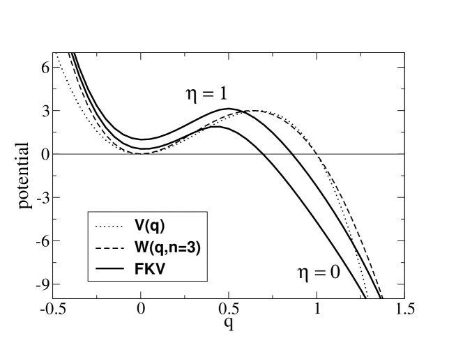
Figure 1: The metastable potentials in one dimension, for a barrier height of $B=3\hbar\varpi$. The coordinate $q$ is given in units of $Q$ and energies are scaled to $\hbar\varpi$. The effective potential $W^{\textrm{FKV}}(\beta,q)$ is shown for $\beta=2\beta_{0}$ and two effective damping strengths $\eta=0$ and $\eta=1$.

In Fig. 1 we show the barrier region of the potentials $V(q)$ and $W(q,n=3)$ with barrier height $B=3\hbar\varpi$. The global minimum of the potential $W(q,n=3)$ is found at $q_{+}\approx 2.4Q$ (not shown in the figure) and is of value $-W(q_{+})\approx 42\hbar\varpi\gg B$. Because of the large depth of this minimum a thermally activated flux originating from this minimum is strongly suppressed. Also shown in Fig. 1 is the “effective classical potential” [21]

$$W^{\textrm{FKV}}(\beta,q_{0})=W(q_{0})-\frac{1}{\beta}\ \textrm{ln}\,\zeta^{\textrm{FKV}}(\beta,q_{0})$$ (65)

for two effective damping strengths and a given temperature. It is the analog of (6) evaluated in the variational approach and contains quantum corrections $\zeta^{\textrm{FKV}}$, which are taken from (4) with $V$ replaced by $W$. As compared to $W(q_{0})$ the effective classical potential $W^{\textrm{FKV}}(\beta,q_{0})$ has a smaller barrier and slightly smaller stiffnesses at $q_{a}$ and $q_{b}$.

Figure 2: A comparison of different approaches to the decay rate for a particle in a one-dimensional cubic potential with barrier, for zero ($\eta=0$) and critical ($\eta=1$) damping. The arrows point to the $\beta_{0}=1/T_{0}$ where the PSPA breaks down. For more details see text.

In Fig. 2 we show the $\beta$-dependence of the rate formulas in logarithmic representation, for two effective damping strengths. The results of two different calculations are presented. The one denoted by “FKV1” (fully drawn line) is evaluated by using formulas (63) and (64), with the quantum corrections $f_{\textrm{qm}}$ taken from (60) and (4). For the second calculation (“FKV2”, fully drawn line with symbols) the saddle point approximation is applied directly to the effective classical potential (65). The quantal rate is calculated from the formulas

$$R(\beta<\beta_{0}) \!=\! \frac{\sqrt{|(W_{b}^{\textrm{FKV}})^{\prime\prime}|/M}}{2\pi}\left(\sqrt{1+\eta^{2}}-\eta\right)\sqrt{\frac{(W_{a}^{\textrm{FKV}})^{\prime\prime}}{|(W_{b}^{\textrm{FKV}})^{\prime\prime}|}}\,\exp(-\beta B^{\textrm{FKV}})\quad$$ (66)

$$R(\beta>\beta_{0}) = \frac{1}{\hbar\beta}\,\sqrt{\frac{(W_{a}^{\textrm{FKV}})^{\prime\prime}}{|(W_{b}^{\textrm{FKV}})^{\prime\prime}|}}\,\exp(-\beta B^{\textrm{FKV}})\,,$$ (67)

where $B^{\textrm{FKV}}=W_{b}^{\textrm{FKV}}-W_{a}^{\textrm{FKV}}$ is the (temperature-dependent) effective barrier height within the FKV, which is smaller than $B$, as can be seen from Fig. 1. Please note that FKV2 is a less drastic approximation to the $q_{0}$-integral for $\mathcal{Z}$ than FKV1. In addition we show in Fig. 2 the classical rate as a dotted line, for which $f_{\textrm{qm}}^{\textrm{SPA}}\equiv 1$. The analog of the PSPA rate for a particle moving in a one-dimensional potential takes into account quantum effects via a Gaussian approximation. In order to keep the figure transparent these curves are not shown here. The inverse crossover temperature $\beta_{0}=1/T_{0}$, however, where the PSPA formalism breaks down due to a divergence of $f_{\textrm{qm}}^{\textrm{PSPA}}$, is marked by arrows. For low temperatures $\beta>\beta_{0}$ also the result of H. Grabert et al. [4, 5] is plotted (dashed line). Taking from Tab. I and II of [5] the relevant quantities, these results were obtained from an exact numerical treatment of the dynamical “bounce solution” $q_{\textrm{B}}(\tau)$.

The classical decay rate shows the purely exponential behavior known from Arrhenius’ law. The rates derived from FKV1 and FKV2 coincide with the classical result at high temperatures (small $\beta$) but show enhancement at larger $\beta$. In the crossover region $\beta\approx\beta_{0}$ these approximations smoothly connect the classical rate with the result of Grabert et al. for $\beta>\beta_{0}$. For very low temperatures ($\beta\gg\beta_{0}$), however, FKV1 and FKV2 deliver bad results, too. Instead of converging to a finite limit, both versions qualitatively behave more like the classical rate and fall off exponentially. This can be understood as follows: Also the FKV is basically a static approximation that incorporates inharmonic terms by smearing out the potential locally, see Fig. 1. This works well as long as the quantum fluctuations are not too large, as given for moderate to high temperatures. At very low temperatures, however, there is no way around accounting for the full nonlinearity of the dynamical bounce solution $q_{B}(\tau)$, which minimizes the Euclidean action for $\beta>\beta_{0}$ and therefore gives the leading contribution to the decay rate. Due to this limitation of the variational approach, it would simply be asking too much to expect good agreement with the fully quantum rate even at extremely small temperatures. As the FKV2 contains more information about the quantum effects than the FKV1 it underestimates the rate less dramatically at low temperatures. Especially in the region $\beta\gtrsim\beta_{0}$ FKV2 still delivers acceptable results where FKV1 is no longer reliable.

References

- [1] J. S. Langer, Ann. Phys. (N.Y.) 41, 108 (1967); J. S. Langer, Ann. Phys. (N.Y.) 54, 258 (1969).
- [2] A. O. Caldeira and A. J. Leggett, Ann. Phys. 149, 374 (1983), 153, 445(E) (1984).
- [3] A. I. Larkin and Y. N. Ovchinnikov, Pis’ma Zh. Eksp. Teor. Fiz. 37, 322 (1983), [JETP Lett. 37, 382 (1983)]; A. I. Larkin and Y. N. Ovchinnikov, Zh. Eksp. Teor. Fiz. 86, 719 (1984), [Sov. Phys. JETP 59, 420 (1984)].
- [4] H. Grabert, U. Weiss, and P. Hänggi, Phys. Rev. Lett. 52, 2193 (1984); H. Grabert and U. Weiss, Phys. Rev. Lett. 53, 1787 (1984).
- [5] H. Grabert, P. Olschowski, and U. Weiss, Phys. Rev. B 36, 1931 (1987).
- [6] P. Hänggi, P. Talkner, and M. Borkovec, Rev. Mod. Phys. 62, 251 (1990).
- [7] U. Weiss, Quantum Dissipative Systems (World Scientific, Singapore, 1993).
- [8] C. Rummel and H. Hofmann, Phys. Rev. E 64, 066126 (2001).
- [9] G. Puddu, P. F. Bortignon, and R. A. Broglia, Ann. Phys. (San Diego) 206, 409 (1991).
- [10] H. Attias and Y. Alhassid, Nucl. Phys. A 625, 565 (1997).
- [11] R. Rossignoli and N. Canosa, Phys. Lett. B 394, 242 (1997); R. Rossignoli and P. Ring, Nucl. Phys. A 633, 613 (1998).
- [12] C. Rummel, Ph.D. thesis, Technische Universität München, 2004.
- [13] C. Rummel and H. Hofmann, nucl-th/0407092.
- [14] P. Siemens, A. Jensen, and H. Hofmann, in Nucleon-Nucleon Interaction and the Nuclear Many-Body Problem, edited by S. Wu and T. Kuo (World Scientific, Singapore, 1984), p. 231.
- [15] H. Hofmann, Phys. Rep. 284 (4&5), 137 (1997).
- [16] A. Bohr and B. R. Mottelson, Nuclear Structure (Benjamin, London, 1975), Vol. 2.
- [17] R. P. Feynman and A. R. Hibbs, Quantum Mechanics and Path Integrals (Mc Graw Hill, New York, 1965).
- [18] C. Rummel and J. Ankerhold, Eur. Phys. J. B 29, 105 (2002).
- [19] C. Mahaux and R. Sartor, in Advances in nuclear physics, edited by J. Negele and E. Vogt (Plenum Press, New York, 1991), Vol. 20.
- [20] G. E. Brown and M. Rho, Nucl. Phys. A 372, 397 (1981).
- [21] R. P. Feynman and H. Kleinert, Phys. Rev. A 34, 5080 (1986).
- [22] I. Affleck, Phys. Rev. Lett. 46, 388 (1981).
- [23] H. A. Kramers, Physica (Utrecht) 7, 284 (1940).
- [24] H. J. Lipkin, N. Meshkov, and A. J. Glick, Nucl. Phys. 62, 188 (1965).
- [25] P. Arve, G. F. Bertsch, J. W. Negele and G. Puddu, Phys. Rev. C 36, 2018 (1987).
- [26] H. Kleinert and I. Mustapic, Int. J. Mod. Phys. A 11, 4383 (1996).