Surface Partition of Large Fragments

Abstract

The surface partition of large fragments is derived analytically within a simple statistical model by the Laplace-Fourier transformation method. In the limit of small amplitude deformations, a suggested Hills and Dales Model reproduces the leading term of the famous Fisher result for the surface entropy with an accuracy of a few percent. The surface partition of finite fragments is discussed as well.

I Introduction

During last forty years the Fisher droplet model (FDM) Fisher:64 , on one hand, was extensively used to analyze the condensation of gaseous phase (droplets of all sizes) into liquid. The gaseous phases are ranging from mixture of nuclear fragments Moretto to the various clusters on 2- and 3-dimensional Ising lattices Ising:clust . On the other hand, the FDM inspired the formulation of a more sophisticated model, the statistical multifragmentation model (SMM) Bondorf:95 , which describes not only the gaseous phase of nuclear fragments, but the liquid phase (nuclear matter) as well on the same footing Bugaev:00 ; Bugaev:01 ; Reuter:01 .

Applying the FDM to the nuclear fragment of $A$-nucleons, one can cast its free-energy $F_{A}$ as follows

$$F_{A}=-W~{}A+\sigma(T)~{}A^{2/3}+\tau T\ln A~{}$$ (1)

Here $W$ is the bulk binding energy per nucleon, $\sigma(T)$ is the temperature dependent surface tension which about the critical temperature $T_{c}$ is parameterized in the following form: $\sigma(T)=\sigma_{\rm o}[1~{}-~{}T/T_{c}],$ with $\sigma_{\rm o}\approx 18$ MeV and $T_{c}=18$ MeV ($\sigma=0$ at $T\geq T_{c}$). The last contribution in Eq. (1) generates the famous Fisher’s term with dimensionless parameter $\tau$. From the study of the combinatorics of lattice gas clusters in two dimensions, Michael Fisher had postulated Eq. (1) and this kind of temperature dependence of the surface tension because the latter naturally leads to the existence of critical temperature $T_{c}$. This is, of course, not a unique parametrization of the surface tension. The SMM, for instance, successfully employs another one Bondorf:95 $\sigma(T)=\sigma_{\rm o}[(T_{c}^{2}~{}-~{}T^{2})/(T_{c}^{2}~{}+~{}T^{2})]^{5/4}.$ Therefore, it is necessary to study a few simple, but quite fundamental questions, “What is the origin of the Fisher parametrization for the temperature dependent surface tension in three dimensions? Does any physical motivation favor the Fisher parametrization?” This work is devoted to these questions of fundamental importance.

II Hills and Dales Model

To answer these main questions we will consider the statistical model of surface deformations. We will, however, impose a necessary constraint that the deformations should conserve the total volume of the fragment of $A$-nucleons. As we will see, the most interesting result corresponds to the deformations of vanishing amplitude. Therefore, it is clear that the shape of deformation cannot be important and we can choose one which is regular to simplify our presentation. For this reason we shall consider cylindrical deformations of positive height $h_{k}>0$ (hills) and negative height $-h_{k}$ (dales), with $k$ nucleons at the base. For simplicity it is assumed that the top (bottom) of the hill (dale) has the same shape as the surface of original fragment of $A$ nucleons. Our main assumptions are as follows: (i) the statistical weight of deformations $\exp\left(-\sigma_{\rm o}|\Delta S_{k}|/T/s_{1}\right)$ is given by the Boltzmann factor due to the change of the surface $|\Delta S_{k}|$ in units of the surface per one nucleon $s_{1}$; (ii) the hill’s heights $h_{k}\leq H_{k}$ ($H_{k}$ is the maximal height of the hill with $k$ nucleons at the base) have the same probability $dh_{k}/H_{k}$ besides the statistical one; (iii) the same two assumptions are valid for the dales as well. As we will see, these assumptions are not too restrictive, but allow us to simplify the analysis.

Under adopted assumptions it is possible to find the one-particle statistical partition of the deformation of the $k$ nucleons base as a convolution of two probabilities:

$$z_{k}^{\pm}\equiv\int\limits_{0}^{\pm H_{k}}\frac{dh_{k}}{\pm H_{k}}\,{\textstyle e^{-\frac{\sigma_{\rm o}P_{k}|h_{k}|}{Ts_{1}}}}=Ts_{1}\frac{\left[1-{\textstyle e^{-\frac{\sigma_{\rm o}P_{k}H_{k}}{Ts_{1}}}}\right]}{\sigma_{\rm o}P_{k}H_{k}}\,,$$ (2)

where upper (lower) sign corresponds to hills (dales). Here $P_{k}$ is the perimeter of the cylinder base. Now we have to find a geometrical partition (degeneracy factor) or the number of ways to place the center of a given deformation on the surface of $A$-nucleon fragment while it is occupied by the set of $\{n_{l}^{\pm}=0,1,2,...\}$ deformations of the $l$ nucleons base. Our next assumption is that the desired geometrical partition can be given in the excluded volume approximation

$${\cal G}=\frac{S_{A}-\sum\limits_{k=1}^{K_{max}}k\,(n_{k}^{+}~{}+~{}n_{k}^{-})\,s_{1}}{s_{1}}\,,$$ (3)

where $s_{1}k$ is the area occupied by the deformation of $k$ nucleon base ($k=1,2,...$), $S_{A}$ is the full surface of the fragment, and $K_{max}(S_{A})$ is the $A$-dependent size of the maximal allowed base on the fragment. It is clearly seen now that the denominator in the right hand side (r.h.s.) of (3) corresponds to the available surface to place the center of each of $\{n_{k}^{\pm}\}$ deformations that exist on the fragment surface. It is necessary to impose the condition ${\cal G}\geq 0$ which ensures that the deformations do not overlap on the available surface of the fragment. Eq. (3) is the Van der Waals excluded volume approximation usually used in statistical mechanics at not too high particle densities Bondorf:95 ; Bugaev:00 ; Goren:81 and it can be derived for the objects of different sizes in a spirit of a method proposed in Zeeb:02 .

According to Eq. (2) the statistical partition for the hill with a $k$-nucleon base matches that of the dale, i.e. $z^{+}_{k}=z^{-}_{k}$. Therefore, the grand canonical surface partition (GCSP)

$$Z(S_{A})=\sum\limits_{\{n_{k}^{\pm}=0\}}^{\infty}\left[\prod_{k=1}^{K_{max}}\frac{\left[z_{k}^{+}{\cal G}\right]}{n^{+}_{k}!}^{n^{+}_{k}}\frac{\left[z_{k}^{-}{\cal G}\right]}{n^{-}_{k}!}^{n^{-}_{k}}\right]\Theta(s_{1}{\cal G})\,$$ (4)

corresponds to the conserved (on average) volume of the fragment because the probabilities of hill and dale of the same base are identical. The presence of $\Theta(s_{1}{\cal G})$-function in (4) ensures that only configurations with positive value of the free surface of fragment are taken into account. However, this makes the calculation of the GCSP very difficult. Because of the explicit $S_{A}$ dependence of the maximal base of deformations via $K_{max}(S_{A})$ the standard trick to deal with the excluded volume partitions, the usual Laplace transform method Goren:81 ; Bugaev:00 ; Bugaev:01 in $S_{A}$, cannot overcome this difficulty. However, the GCSP (4) can be solved with the help of the recently developed Laplace-Fourier technique Bugaev:04 . The latter employs the identity

$$G(S_{A})=\int\limits_{-\infty}^{+\infty}d\xi~{}\int\limits_{-\infty}^{+\infty}\frac{d\eta}{\sqrt{2\pi}}~{}{\textstyle e^{i\eta(S_{A}-\xi)}}~{}G(\xi)\,,$$ (5)

which is based on the Fourier representation of the Dirac $\delta$-function. The representation (5) allows us to decouple the additional $S_{A}$-dependence in $K_{max}(S_{A})$ and reduce it to the exponential one, which can already be integrated by the Laplace transform Bugaev:04

$${\cal Z}(\lambda)~{}\equiv~{}\int_{0}^{\infty}dS_{A}~{}{\textstyle e^{-\lambda S_{A}}}~{}{Z}(S_{A})=$$

$$\int_{0}^{\infty}dS^{\prime}\int\limits_{-\infty}^{+\infty}d\xi~{}\int\limits_{-\infty}^{+\infty}\frac{d\eta}{\sqrt{2\pi}}~{}{\textstyle e^{i\eta(S^{\prime}-\xi)-\lambda S^{\prime}}}\sum\limits_{\{n_{k}^{\pm}=0\}}^{\infty}\left[\prod_{k=1}^{K_{max}(\xi)}\right.$$

$$\left.\frac{\left[z_{k}^{+}S^{\prime}{\textstyle e^{k\,s_{1}(i\eta-\lambda)}}\right]}{n^{+}_{k}!~{}s_{1}^{n^{+}_{k}}}^{n^{+}_{k}}\frac{\left[z_{k}^{-}S^{\prime}{\textstyle e^{k\,s_{1}(i\eta-\lambda)}}\right]}{n^{-}_{k}!~{}s_{1}^{n^{-}_{k}}}^{n^{-}_{k}}\right]\Theta(S^{\prime})=$$

$$\int_{0}^{\infty}dS^{\prime}\int\limits_{-\infty}^{+\infty}d\xi~{}\int\limits_{-\infty}^{+\infty}\frac{d\eta}{\sqrt{2\pi}}~{}{\textstyle e^{i\eta(S^{\prime}-\xi)-\lambda S^{\prime}+S^{\prime}{\cal F}(\xi,\lambda-i\eta)}}\,.$$ (6)

After changing the integration variable $S_{A}\rightarrow S^{\prime}=S_{A}-\sum\limits_{k=1}^{K_{max}(\xi)}k\,(n_{k}^{+}~{}+~{}n_{k}^{-})\,s_{1}$, the constraint of $\Theta$-function has disappeared. Then all $n_{k}$ were summed independently leading to the exponential function. Now the integration over $S^{\prime}$ in (II) can be straightforwardly done resulting in

$${\cal Z}(\lambda)=\int\limits_{-\infty}^{+\infty}d\xi\int\limits_{-\infty}^{+\infty}\frac{d\eta}{\sqrt{2\pi}}~{}\frac{\textstyle e^{-i\eta\xi}}{{\textstyle\lambda-i\eta~{}-~{}{\cal F}(\xi,\lambda-i\eta)}}~{},$$ (7)

where the function ${\cal F}(\xi,\tilde{\lambda})$ is defined as follows

$${\cal F}(\xi,\tilde{\lambda})=\sum\limits_{k=1}^{K_{max}(\xi)}\left[\frac{z_{k}^{+}}{s_{1}}+\frac{z_{k}^{-}}{s_{1}}\right]~{}e^{-k\,s_{1}\tilde{\lambda}}\,.$$ (8)

As usual, in order to find the GCSP by the inverse Laplace transformation, it is necessary to study the structure of singularities of the partition (7). Since the HDM requires the fragment volume conservation, hereafter we will call (7) as an isochoric partition or isochoric ensemble.

III Isochoric Ensemble Singularities

For finite fragment surface the structure of singularities of the isochoric partition (7) can be complicated. To see this let us first make the inverse Laplace transform:

$$Z(S_{A})~{}=\int\limits_{\chi-i\infty}^{\chi+i\infty}\frac{d\lambda}{2\pi i}~{}{\cal Z}(\lambda)~{}e^{\textstyle\lambda\,S_{A}}=$$

$$\int\limits_{-\infty}^{+\infty}d\xi\int\limits_{-\infty}^{+\infty}\frac{d\eta}{\sqrt{2\pi}}\int\limits_{\chi-i\infty}^{\chi+i\infty}\frac{d\lambda}{2\pi i}~{}\frac{\textstyle e^{\lambda\,S_{A}-i\eta\xi}}{{\textstyle\lambda-i\eta~{}-~{}{\cal F}(\xi,\lambda-i\eta)}}~{}=$$

$$\int\limits_{-\infty}^{+\infty}d\xi\int\limits_{-\infty}^{+\infty}\frac{d\eta}{\sqrt{2\pi}}\,{\textstyle e^{i\eta(S_{A}-\xi)}}\sum_{\{\tilde{\lambda}_{n}\}}e^{\textstyle\tilde{\lambda}_{n}\,S_{A}}{\textstyle\left[1-\frac{\partial{\cal F}(\xi,\tilde{\lambda}_{n})}{\partial\tilde{\lambda}_{n}}\right]^{-1},}$$ (9)

where the contour integral in $\lambda$ is reduced to the sum over the residues of all singular points $\lambda=\tilde{\lambda}_{n}+i\eta$ with $n=0,1,2,..$, since this contour in the complex $\lambda$-plane obeys the inequality $\chi>\max(Re\{\tilde{\lambda}_{n}\})$. Now all integrations in (III) can be done, and the GCSP acquires the form

$$Z(S_{A})~{}=\sum_{\{\tilde{\lambda}_{n}\}}e^{\textstyle\tilde{\lambda}_{n}\,S_{A}}\left[1-\frac{\partial{\cal F}(S_{A},\tilde{\lambda}_{n})}{\partial\tilde{\lambda}_{n}}\right]^{-1}\,,$$ (10)

i.e. the double integral in (III) simply reduces to the substitution $\xi\rightarrow S_{A}$ in the sum over singularities. This remarkable answer is a partial example of the general theorem on the Laplace-Fourier transformation properties proved in Bugaev:04 .

The simple poles in (III) are defined by the condition $\tilde{\lambda}_{n}~{}=~{}{\cal F}(S_{A},\tilde{\lambda}_{n})$ and the latter can be cast as a system of two coupled transcendental equations

$$R_{n}=~{}\sum\limits_{k=1}^{K_{max}(S_{A})}\left[z_{k}^{+}+z_{k}^{-}\right]~{}{\textstyle e^{-k\,R_{n}}}\cos(I_{n}k)\,,$$ (12)

$$I_{n}=-\sum\limits_{k=1}^{K_{max}(S_{A})}\left[z_{k}^{+}+z_{k}^{-}\right]~{}{\textstyle e^{-k\,R_{n}}}\sin(I_{n}k)\,,$$

for dimensionless variables $R_{n}=s_{1}Re(\tilde{\lambda}_{n})$ and $I_{n}=s_{1}Im(\tilde{\lambda}_{n})$. So far Eqs. (12) and (12) are rather general and can be used for particular models which specify the height of hills and depth of dales. But we can give an absolute supremum for the real root $(R_{0};I_{0}=0)$ of these equations. For this purpose it is sufficient to consider the limit $K_{max}(S_{A})\rightarrow\infty$, because for $I_{n}=I_{0}=0$ the right hand side (r.h.s.) of (12) is a monotonously increasing function of $K_{max}(S_{A})$. Since $z_{k}^{+}=z_{k}^{-}$ are the monotonously decreasing functions of $H_{k}$, the maximal value of the r.h.s. of (12) corresponds to the limit of infinitesimally small amplitudes of deformations, $H_{k}\rightarrow 0$. Under these conditions Eq. (12) for $I_{n}=I_{0}=0$ becomes an identity and Eq. (12) acquires the form

$$R_{0}\rightarrow~{}2\sum\limits_{k=1}^{\infty}e^{-\frac{\sigma_{\rm o}P_{k}H_{k}}{2Ts_{1}}}~{}{\textstyle e^{-k\,R_{0}}}=2\left[e^{R_{0}}-1\right]^{-1}\,,$$ (13)

and we have $R_{0}=s_{1}\tilde{\lambda}_{0}\approx 1.06009$. Since for $I_{n}\neq 0$ defined by (12) the inequality $\cos(I_{n}k)\leq 1$ cannot become the equality for all values of $k$ simultaneously, then it follows that the real root of (12) obeys the inequality $R_{0}>R_{n>0}$. The last result means that in the limit of infinite fragment, $S_{A}\rightarrow\infty$, the GCSP is represented by the farthest right singularity among all simple poles $\{\tilde{\lambda}_{n}\}$

$$Z(S_{A})\biggl{|}_{S_{A}\rightarrow\infty}~{}\approx\frac{e^{\textstyle\frac{R_{0}\,S_{A}}{s_{1}}}}{1+\frac{R_{0}^{2}}{2}}\approx 0.6402~{}e^{\textstyle\frac{R_{0}\,S_{A}}{s_{1}}}$$ (14)

There are two remarkable facts regarding (14): first, this result is model independent because in the limit of vanishing amplitude of deformations all specific parameters of the model have dropped out; second, in evaluating (14) we did not specify the shape of the fragment under consideration, but only implicitly required that the fragment surface together with deformations is a regular surface without self-intersections. Therefore, for vanishing amplitude of deformations the latter means that Eq. (14) should be valid for any self-non-intersecting surfaces.

For spherical fragments the r.h.s. of (14) becomes familiar, $0.6402~{}e^{\textstyle 1.06009\,A^{2/3}}$, which, combined with the Boltzmann factor of the surface energy $e^{\textstyle-\sigma_{\rm o}A^{2/3}/T}$, generates the following temperature dependent surface tension of the large fragment

$$\sigma(T)=\sigma_{\rm o}\left[1-1.06009\frac{T}{\sigma_{\rm o}}\right]$$ (15)

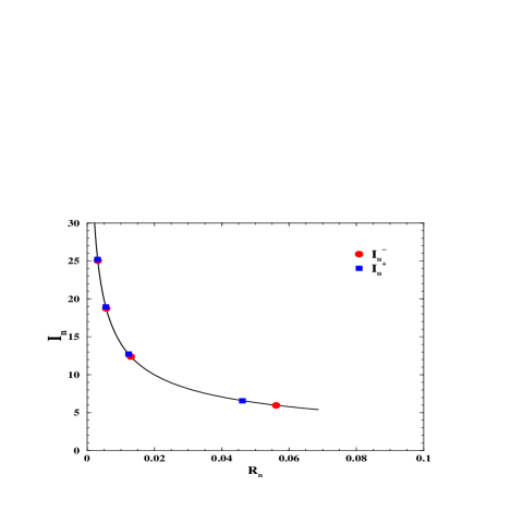
Figure 1: The first quadrant of the complex plane $s_{1}\tilde{\lambda}_{n}\equiv R_{n}+iI_{n}$ of the roots of the system of (16) and (17). The circles and squares represent the two branches $I_{n}^{-}$ and $I_{n}^{+}$ of the roots, respectively. The curve is defined by the approximation given by (19) and (20) (see text for more details).

which means that the actual critical temperature of the three dimensional Fisher model should be $T_{c}=\sigma_{\rm o}/1.06009$, i.e. 6 % smaller than Fisher originally supposed. Note please that this equation for the critical temperature remains valid for the temperature dependent $\sigma_{\rm o}$ as well. It is also surprising that the degeneracy factor $0.6402$ in (14) is only 12.5 % larger than the corresponding factor of the self-avoiding polygons on the two-dimensional square lattice SAP .

For the large, but finite fragments it is necessary to take into account not only the farthest right singularity $\tilde{\lambda}_{0}=R_{0}/s_{1}$ in (10), but all other roots with positive real part $R_{n>0}>0$. In this case for each $R_{n>0}$ there are two roots $\pm I_{n}$ of (12) because the GCSP is real by definition. The roots of Eqs. (12) and (12) with largest real part are very insensitive to the large values of $K_{max}(S_{A})$, therefore, it is sufficiently good to keep $K_{max}(S_{A})\rightarrow\infty$. Then for limit of vanishing amplitude of deformations Eqs. (12) and (12) can be, respectively, rewritten as

$$\frac{2R_{n}}{R_{n}^{2}+I_{n}^{2}}=~{}~{}{\textstyle e^{R_{n}}}\cos(I_{n})-1\,,$$ (16)

$$\frac{2I_{n}}{R_{n}^{2}+I_{n}^{2}}=-~{}{\textstyle e^{R_{n}}}\sin(I_{n})\,.$$ (17)

After some algebra the system of (16) and (17) can be identically reduced to a single equation for $R_{n}$

$$\cos\left({\textstyle\left[\frac{4(1+R_{n})}{e^{2R_{n}}-1}-R_{n}^{2}\right]^{1/2}}\right)=\cosh R_{n}-\frac{\sinh R_{n}}{1+R_{n}}\,,$$ (18)

and the quadrature $I_{n}^{2}=\sqrt{\frac{4(1+R_{n})}{e^{2R_{n}}-1}-R_{n}^{2}}$. The analysis shows that besides the opposite signs there are two branches of solutions, $I^{+}_{n}$ and $I^{-}_{n}$, for the same $n\geq 1$ value:

$$|I^{\pm}_{n}| \approx 2\pi n\pm\frac{1}{\pi n}\,,$$ (19)

$$R_{n} \approx \pi^{2}n^{2}+1-\pi n\sqrt{\pi^{2}n^{2}+2}\,.$$ (20)

The exact solutions $(R_{n};I^{\pm}_{n})$ for $n>1$ which have the largest real part are shown in Fig. 1. together with the curve parametrized by functions $I_{x}^{+}$ and $R_{x}$ taken from Eqs. (19) and (20), respectively. From Eq. (20) and Fig. 1. it is clearly seen that the largest real part $R_{1}\approx 0.0582$ is about 18 times smaller than $R_{0}$, and, therefore, already for the fragment of a few nucleons the correction to the leading term (14) is exponentially small. Using the approximations (19) and (20), for $n>2$ one can estimate

$$\biggl{|}{\textstyle e^{\tilde{\lambda}_{n}\,S_{A}}\left[1-\frac{\partial{\cal F}(S_{A},\tilde{\lambda}_{n})}{\partial\tilde{\lambda}_{n}}\right]^{-1}}\biggr{|}\leq e^{\textstyle\frac{S_{A}}{2\pi^{2}n^{2}s_{1}}}~{}/~{}(2\pi^{2}n^{2})$$ (21)

the upper limit of the $(R_{n};I^{\pm}_{n})$ root contribution into the GCSP (10). This result shows that the total contribution of all complex poles in (10) is negligibly small compared to the leading term (14) for a fragment of a few nucleons already. The latter, however, requires a more careful accounting for the volume conservation of a fragment.

IV Concluding Remarks

The developed model allows us to give the upper limit for the surface entropy because it corresponds to the vanishing amplitude of deformations and, therefore, the specific features of the model were irrelevant for our analysis. To find the next order correction to the surface entropy one has already to consider the underlying model for deformations. We, however, would like to show how the power law may arise within the HDM. For this purpose let us consider the left equality in (13) which is valid for small heights of deformations. It can be shown that the following ansatz $(S_{A}>>s_{1})$ for the deformation energy

$$\frac{\sigma_{\rm o}P_{k}H_{k}}{2Ts_{1}}\rightarrow-\frac{3}{2}~{}k~{}\tau{\textstyle\left[1+\frac{2}{R_{0}(2+R_{0})}\right]}~{}\frac{s_{1}}{S_{A}}\ln\left(\frac{s_{1}}{S_{A}}\right)$$ (22)

of $k$ nucleon base, indeed, generates the Fisher power law $A^{-\tau}$ for the GCSP (14) of an $A$-nucleon fragment. From (22) it is clearly seen that the term $-k\frac{s_{1}}{S_{A}}\ln\left(\frac{s_{1}}{S_{A}}\right)$ is the entropy which gives an a priori uncertainty to measure the position of $k$ nucleons of area $s_{1}$ on the surface of the fragment. A comparison of (22) with any $kR_{n}>0$ in the left equality (13) shows that in the limit $S_{A}>>s_{1}$ the ansatz (22) corresponds to a negligible correction compared to the exponentials $e^{\frac{R_{n}S_{A}}{s_{1}}}$. Therefore, the Fisher power law is too delicate for the model developed to study the surface partition of large fragments.

In conclusion, we developed a simple statistical model which allowed us to derive analytically the general expression (10) for the GCSP. This result is achieved by the Laplace-Fourier transformation technique to the isochoric ensemble. We named this ensemble because the HDM obeys the volume conservation of a fragment under consideration. The volume conservation is accounted for by the equal statistical probabilities for the hills and dales of the same base. The limit of vanishing deformations allowed us to find a supremum for the surface entropy of the large fragments which, remarkably, exceeds the Fisher original assumption by only 6 percent. The analytical analysis of the corrections to the GCSP (14) originating from the complex roots of Eqs. (12) and (12) showed that these corrections are negligible already for the fragment of a few nucleons. The HDM allows one to study the statistical mechanics of volume deformations of finite or even small fragments, but this task requires further refinements of the model.

Acknowledgments. This work was supported by the US Department of Energy.

References

- (1) M.E. Fisher, Physics 3 (1967) 255.
- (2) L. G. Moretto et. al., Phys. Rep. 287 (1997) 249.
- (3) C. M. Mader et al., Phys. Rev. C 68 (2003) 064601.
- (4) J. P. Bondorf et al., Phys. Rep. 257 (1995) 131.
- (5) K. A. Bugaev et. al., Phys. Rev. C62 (2000) 044320; arXiv:nucl-th/0007062 (2000).
- (6) K. A. Bugaev et. al., Phys. Lett. B 498 (2001) 144; arXiv:nucl-th/0103075 (2001).
- (7) P. T. Reuter and K. A. Bugaev, Phys. Lett. B 517 (2001) 233.
- (8) M. I. Gorenstein, V. K. Petrov and G. M. Zinovjev, Phys. Lett. B 106 (1981) 327.
- (9) G. Zeeb, K. A. Bugaev, P. T. Reuter and H. Stocker, arXiv:nucl-th/0209011.
- (10) K. A. Bugaev, arXiv:nucl-th/0406033.
- (11) I. Jensen and A. J. Guttmann, J. Phys. A 32 (1999) 4867.