Method of multiple internal reflections in description of tunneling evolution through barriers

A method of a non-stationary description of tunneling of a particle through the one-dimensional and spherically symmetric rectangular barriers on the basis of analisis of multiple internal reflections of wave packets in relation on the barrier boundaries, named as the method of multiple internal reflections, is presented at the first time. For the one-dimensional problem the applicability of this method is proved, its specific features are analyzed. For the spherically symmetric problem the amplitudes of the transmitted and reflected wave packets, times of tunneling and reflection in relation to the barrier are calculated using this method. The effect of Hartman-Fletcher is analyzed.

PACS numbers: 03.65.-w, 03.65.Nk, 03.65.Xp,

UDC 539.14

Keywords: 1D- and 3D-tunneling, multiple internal reflections, spherically symmetric elastic scattering, transmission and reflection coefficients, wave packet, tunneling times, effect of Hartman-Fletcher

1 Introduction

As the further development of the time analysis of tunneling processes considered in [1, 2, 3], here we present the non-stationary solution method for the problem of scattering of nonrelativistic particle on the spherically symmetric field which has rectangular barrier. Such approach uses the account of multiple internal reflections of fluxes in relation to the boundaries of the barrier (this approach further we name as the method of multiple internal reflections and we present such a method at the first time).

An important specific feature of this method is a consideration of particle propagation on the basis of wave packets (WPs). Due to this one can fulfill the time analysis of particle propagation (or tunneling) and study in details these processes in interesting time moment or in relation to the concrete point of space. In result, the validation of method on the basis of the account of the multiple internal reflections of WP is given correctly both for above-barrier and sub-barrier regions (unlike stationary consideration of such approach to the problem solution [4, 5]).

At the beggining we consider the problem of tunneling of particle through an one-dimensional rectangular barrier. This problem is test one and allows to analyze the specific features of this method. The time analysis of the method of multiple internal reflections is fulfilled for the first time.

The interesting perspective of this method is enough easy calculation (in comparison with the known stationary methods) of stationary wave functions (WFs) for the one-dimensional and spherically symmetric problems with barriers of more composite form than rectangular. It is shown weakly in the one-dimensional problem with one rectangular barrier and is shown more brightly in the problems with barriers of more composite forms. As an example we consider the one-dimensional problem with the double-humb rectangular barrier.

Further the method is used for solving the problem of scattering of particle on the spherically symmetric field, which radial part has a rectangular barrier. For it the amplitudes of transmitted and reflected WPs, total times of tunneling and reflection in relation to the barrier are found. The effect of Hartman - Fletcher is considered. The expression for the S-matrix is presented in the form of the sum of two components corresponding to the amplitudes of transmitted and reflected WPs. Spherically symmetric problem with use of the method of multiple internal reflections is solved for the first time.

2 The tunneling evolution of particle through the 1D- rectangular barrier

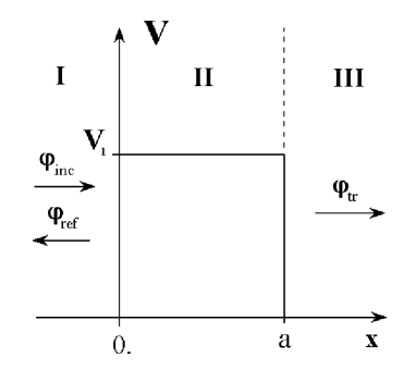
Fig. 1: An one-dimension one-humb rectangular barrier

Let’s consider the problem of particle moving along the $x$-direction and tunneling through a rectangular potential barrier (see Fig. 1). We label the region I for $x<0$, region II for $0<x<a$ and region III for $x>a$, accordingly. Solving the stationary Schrödinger equations, one can find the general solution for WF:

$$\varphi(x)=\left\{\begin{array}[]{ll}e^{ikx}+A_{R}e^{-ikx},&\mbox{for }x<0;\\ \alpha e^{-\xi x}+\beta e^{\xi x},&\mbox{for }0<x<a;\\ A_{T}e^{ikx},&\mbox{for }x>a;\end{array}\right.$$ (1)

where $k=\frac{1}{\hbar}\sqrt{2mE}$, $\xi=\frac{1}{\hbar}\sqrt{2m(V_{1}-E)}$, $E$ and $m$ are the energy and mass of a particle, accordingly. The coefficients $A_{T}$, $A_{R}$, $\alpha$ and $\beta$ can be calculated analytically, using requirements of the continuity of WF $\varphi(x)$ and its derivative on each boundaries of the barrier.

The tunneling evolution of particle can be described using non-stationary consideration of the propagating WP constructed on the basis of solution of the stationary Schrödinger equations:

$$\psi(x,t)=\int\limits_{0}^{+\infty}g(E-\bar{E})*\varphi(x,k)e^{-iEt/\hbar}dE,$$ (2)

where the weight amplitude $g(E-\bar{E})$ satisfies to the requirement of the normalization $\int|g(E-\bar{E})|^{2}dE=1$, value $\bar{E}$ is the average energy.

By inserting in the integral (2) instead of the total wave $\varphi(x,k)$ the incident $\varphi_{inc}(x,k)$, transmitted $\varphi_{tr}(x,k)$ or reflected part of WF $\varphi_{ref}(x,k)$, defined by expression (1), we obtain the incident, transmitted or reflected WP, respectively. Considering only sub-barrier processes, we exclude the component of waves for above-barrier energies, including the additional transformation:

$$g(E-\bar{E})\to G(E-\bar{E})=g(E-\bar{E})\theta(V_{1}-E).$$ (3)

The method of multiple internal reflections considers the process of WP propagation sequentially on steps of its propagation in relation to each boundary of the barrier.

At the first step we consider WP in region I, which is incident upon the first (initial) boundary of the barrier. Let’s assume, that this packet transforms into the WP, transmitted through this boundary and tunneling further in region II, and into the WP, reflected from boundary and propagating back in region I. Thus from the reasons of elementary causality we consider, that WP, tunneling in region II, is not reached the second (final) boundary of the barrier because of a terminating velocity of its propagation, and consequently at this step we consider only two regions I and II. Because of the same physical reasons to write the expression for this packet, we consider, that its amplitude should decrease in positive $x$-direction. For this we use only one item $\beta*\exp(-\xi x)$ in expression (1), throwing the second increasing item $\alpha*\exp(\xi x)$ (in the opposite case we break the requirement of the finiteness of WF for an indefinitely wide barrier). In result, for the incident, transmitted and reflected WPs in relation to the first boundary one can write:

$$\begin{array}[]{lcll}\psi^{1}_{inc}(x,t)&=&\int\limits_{0}^{+\infty}G(E-\bar{E})*e^{ikx-iEt/\hbar}dE,&x<0,\\ \psi^{1}_{tr}(x,t)&=&\int\limits_{0}^{+\infty}G(E-\bar{E})*\beta^{0}e^{-\xi x-iEt/\hbar}dE&0<x<a,\\ \psi^{1}_{ref}(x,t)&=&\int\limits_{0}^{+\infty}G(E-\bar{E})*A_{R}^{0}e^{-ikx-iEt/\hbar}dE,&x<0.\end{array}$$ (4)

We assume, that during a particular interval of time considered at the first step, the transmitted WP tunnels in the sub-barrier region in the positive $x$-direction. In result, at this step we receive the flux for this packet, not equal to zero. Considering only the stationary expressions for WF for this step, we receive the zero fluxes in the barrier region [4, 5].

Constructing from (4) total WF in regions I and II and using the condition of continuity of this WF and its derivative, we find unknown coefficients $\beta^{0}$ and $A_{R}^{0}$.

At the second step we consider WP, tunneling in region II and incident upon the second boundary of the barrier at point $x=a$. It transforms into the WP, transmitted through this boundary and propagated in region III, and into the WP, reflected from boundary and tunneled back in region II. Let’s define them so:

$$\begin{array}[]{lcll}\psi_{inc}^{2}(x,t)&=&\psi_{tr}^{1}(x,t),&\ 0<x<a,\\ \psi_{tr}^{2}(x,t)&=&\int\limits_{0}^{+\infty}G(E-\bar{E})*A_{T}^{0}e^{ikx-iEt/\hbar}dE,&\ x>a,\\ \psi_{ref}^{2}(x,t)&=&\int\limits_{0}^{+\infty}G(E-\bar{E})*\alpha^{0}e^{\xi x-iEt/\hbar}dE,&\ 0<x<a.\end{array}$$ (5)

Here, for forming the expression for the WP reflected from the boundary, we select the increasing part of stationary solution WF $\alpha^{0}\exp(\xi x)$ only. Imposing the condition of continuity on the time-dependent WF and its derivative at point $x=a$, we obtain 2 new equations, from which we find the unknowns coefficients $A_{T}^{0}$ and $\alpha^{0}$.

At the third step the WP, tunneling in region II, is incident upon the first boundary of the barrier. Then it transforms into the WP, transmitted through this boundary and propagated further in region I, and into the WP, reflected from boundary and tunneled back in region II. For WPs one can write:

$$\begin{array}[]{lcll}\psi_{inc}^{3}(x,t)&=&\psi_{tr}^{2}(x,t),&\ 0<x<a,\\ \psi_{tr}^{3}(x,t)&=&\int\limits_{0}^{+\infty}G(E-\bar{E})*A_{R}^{1}e^{-ikx-iEt/\hbar}dE,&\ x<0,\\ \psi_{ref}^{3}(x,t)&=&\int\limits_{0}^{+\infty}G(E-\bar{E})*\beta^{1}e^{-\xi x-iEt/\hbar}dE,&\ 0<x<a.\end{array}$$ (6)

Using the conditions of continuity for the time-dependent WF and its derivative at point $x=0$, we obtain the unknowns coefficients $A_{R}^{1}$ and $\beta^{1}$.

Analyzing further possible processes of transition (and reflection) of WPs through the boundaries of barrier, we come to a deduction, that any of the following steps can be reduced to one of 3 considered above. For unknown coefficients $\alpha^{i}$, $\beta^{i}$,$A_{T}^{i}$ and $A_{R}^{i}$, used in expressions for WPs, forming in result of some internal reflection from the boundaries, one can obtain the recurrence relations.

Considering the propagation of WP by such way, we obtain the expressions for WF on each region which can be written through the series of multiple WPs. We determine the resultant expressions for the incident, transmitted and reflected WPs in relation to the barrier:

$$\begin{array}[]{lcll}\psi_{inc}(x,t)&=&\int\limits_{0}^{+\infty}G(E-\bar{E})*e^{ikx-iEt/\hbar}dE,&x<0,\\ \psi_{tr}(x,t)&=&\int\limits_{0}^{+\infty}G(E-\bar{E})*\sum\limits_{i=0}^{+\infty}A_{T}^{i}e^{ikx-iEt/\hbar}dE,&x>a,\\ \psi_{ref}(x,t)&=&\int\limits_{0}^{+\infty}G(E-\bar{E})*\sum\limits_{i=0}^{+\infty}A_{R}^{i}e^{-ikx-iEt/\hbar}dE,&x<0.\end{array}$$ (7)

The series of coefficients $\alpha^{n}$, $\beta^{n}$, $A_{T}^{n}$ and $A_{R}^{n}$ can be calculated on the basis of obtained reccurence relations and have the following form:

$$\begin{array}[]{lcllcl}\sum\limits_{n=0}^{+\infty}A_{T}^{n}&=&\displaystyle\frac{i4k\xi e^{-\xi a-ika}}{F_{sub}},&\sum\limits_{n=0}^{+\infty}\alpha^{n}&=&\displaystyle\frac{2k(i\xi-k)e^{-2\xi a}}{F_{sub}},\\ \sum\limits_{n=0}^{+\infty}A_{R}^{n}&=&\displaystyle\frac{k_{0}^{2}*D_{-}}{F_{sub}},&\sum\limits_{n=0}^{+\infty}\beta^{n}&=&\displaystyle\frac{2k(i\xi+k)}{F_{sub}},\end{array}$$ (8)

where

$$\begin{array}[]{lll}F_{sub}&=&(k^{2}-\xi^{2})D_{-}+2ik\xi D_{+},\\ D_{\pm}&=&1\pm e^{-2\xi a},\\ k_{0}^{2}&=&k^{2}+\xi^{2}=\displaystyle\frac{2mV_{1}}{\hbar^{2}}.\end{array}$$ (9)

All obtained expressions for the series $\sum\alpha^{n}$, $\sum\beta^{n}$, $\sum A_{T}^{n}$ and $\sum A_{R}^{n}$ coincide with the corresponding coefficients $\alpha$, $\beta$, $A_{T}$ and $A_{R}$ of the expressions (1), calculated by the stationary methods [2, 6]. Using following substitution

$$i\xi\to k_{2},$$ (10)

where $k_{2}=\frac{1}{\hbar}\sqrt{2m(E-V_{1})}$ is the wave number for the case of above-barrier energies, expression for coefficients $\alpha^{n}$, $\beta^{n}$, $A_{T}^{n}$ and $A_{R}^{n}$ for each step, expressions for WF for each step, the total WP transforms into the corresponding expressions for the problem of the particle propagation above this barrier. Besides the following property is fulfilled:

$$\biggl{|}\sum\limits_{n=0}^{+\infty}A_{T}^{n}\biggr{|}^{2}+\biggl{|}\sum\limits_{n=0}^{+\infty}A_{R}^{n}\biggr{|}^{2}=1.$$ (11)

3 Tunneling and reflecting times

Let’s find the time of leaving of WP from the barrier formed in result of $n$ reflections from the boundaries (we name such WP as $n$-fold packet). Using the expressions (4) for the first step, one can determine the equation describing the propagation of the maximum (peak) for incident, transmitted and reflected WPs in relation to the first boundary:

$$\frac{\partial}{\partial E}arg\psi_{inc}(x,t)=\displaystyle\frac{\partial}{\partial E}arg\psi_{tr}(x,t)=\displaystyle\frac{\partial}{\partial E}arg\psi_{ref}(x,t)=const.$$ (12)

Let the WP in region I be incident upon the first boundary of the barrier in the initial time moment $t_{inc}$. One can find the time $t_{ref}^{1}$ of the leaving of the reflected WP from the first boundary to region I:

$$\begin{array}[]{lcl}t_{ref}^{1}&=&t_{inc}+\hbar\displaystyle\frac{\partial argA_{R}^{0}}{\partial E}=t_{inc}+\displaystyle\frac{2m}{\hbar k\xi}.\end{array}$$ (13)

Similarly, for the time $t_{tr}^{1}$ of the leaving of the transmitted WP from this boundary to region II we receive:

$$\begin{array}[]{lcl}t_{tr}^{1}&=&t_{inc}+\hbar\displaystyle\frac{\partial arg\beta^{0}}{\partial E}=t_{inc}+\displaystyle\frac{m}{\hbar k\xi}.\end{array}$$ (14)

Further we consider the second step, when the WP transits through the second boundary of the barrier at point $x=a$. Using the equations (5) and (12), one can obtain the time of the leaving of the transmitted WP to region III and reflected WP to region II from the second boundary:

$$\begin{array}[]{lcl}t_{tr}^{2}&=&t_{inc}+\displaystyle\frac{ma}{\hbar k}+\hbar\displaystyle\frac{\partial argA_{T}^{0}}{\partial E}=t_{inc}+\displaystyle\frac{2m}{\hbar k\xi},\\ t_{ref}^{2}&=&t_{inc}+\hbar\displaystyle\frac{\partial arg\alpha^{0}}{\partial E}=t_{inc}+\displaystyle\frac{3m}{\hbar k\xi}.\end{array}$$ (15)

Using this approach further, we find the time of the leaving of the $n$-fold WP from the second boundary to region III for the even step $n$:

$$\begin{array}[]{lcl}t_{tr}^{n}&=&t_{inc}+\displaystyle\frac{ma}{\hbar k}+\hbar\displaystyle\frac{\partial argA_{T}^{n}}{\partial E}=t_{inc}+(2n+1)\displaystyle\frac{2m}{\hbar k\xi}.\end{array}$$ (16)

Similarly, for the odd step $n$ (except for first step) we find the time of an leaving of the $n$-fold WP from the first boundary to region I:

$$t_{ref}^{n}=t_{inc}+\hbar\displaystyle\frac{\partial argA_{R}^{n}}{\partial E}=t_{inc}+(n+1)\displaystyle\frac{4m}{\hbar k\xi}.$$ (17)

The complete WF, describing a particle transmitted through barrier, represents total WP, the coordinates $(x,t)$ of maximum of which can be identified with coordinates of a particle (its most probable position), transmitted through the barrier and propagated further in region III. The time corresponding to the leaving of this maximum one can identify with the phase tunneling time of particle through the barrier. One can obtain:

$$\begin{array}[]{lcl}\tau_{tun}^{Ph}&=&t_{tr}-t_{inc}=\displaystyle\frac{ma}{\hbar k}+\hbar\displaystyle\frac{\partial arg\sum\limits_{n=0}^{+\infty}A_{T}^{n}}{\partial E}=\\ &=&\displaystyle\frac{m}{\hbar k\xi}*\displaystyle\frac{k_{0}^{4}sh(2\xi a)+2a\xi k^{2}(\xi^{2}-k^{2})}{4k^{2}\xi^{2}+k_{0}^{4}sh^{2}(\xi a)}.\end{array}$$ (18)

The phase time of reflection of a particle from the barrier takes into account only all WPs leaving from the barrier in region I:

$$\tau_{ref}^{Ph}=t_{ref}-t_{inc}=\hbar\displaystyle\frac{\partial arg\sum\limits_{n=0}^{+\infty}A_{R}^{n}}{\partial E}=\tau_{tun}^{Ph}.$$ (19)

Considering high enough (and wide enough) barrier (limit: $\xi a\gg 1$), one can obtain the following expression for the phase times of tunneling and reflection [2]:

$$\tau_{tun}^{Ph}=\tau_{ref}^{Ph}\to\displaystyle\frac{2}{v\xi},$$ (20)

where $v=\hbar k/m$ is the group velocity. One can see, that these times at such limit coincide with time of reflection $t_{ref}^{1}$ at the first step and with time of transition $t_{tr}^{2}$ at the second step. Therefore, considering $n$-fold transmitted and reflected WPs at such limit the maximum of total WP is determined by first packets only.

The phase times of tunneling and reflection, calculated using of the method of multiple internal reflections, convergent with results of [2].

4 The particle tunnels through the 1D- double-humb rectangular barrier

The method of multiple internal reflections allows simply enough to calculate the amplitudes of transmitted and reflected WPs in relation to the barrier for normalized incident WP, if the general stationary solutions of WF are known. This method is effective in finding the amplitudes for stationary WF. The solutions obtained by this method for the problem with barriers of more composite form, than rectangular, appear easier, than solutions obtained by stationary methods.

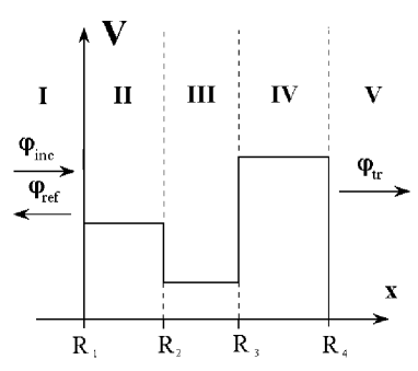
Fig. 2: An one-dimension double-humb rectangular barrier

Let’s consider the particle propagating above the one-dimensional double-humb rectangular barrier (see Fig. 2). Solving the stationary Schrödinger equations in each region, one can obtain the general solution for stationary WF:

$$\varphi(x)=\left\{\begin{array}[]{ll}e^{ikx}+A_{R}e^{-ikx},&\mbox{for }x<R_{1},\\ \alpha_{2}e^{-ik_{2}x}+\beta_{2}e^{ik_{2}x},&\mbox{for }R_{1}<x<R_{2},\\ \alpha_{3}e^{-ik_{3}x}+\beta_{3}e^{ik_{3}x},&\mbox{for }R_{2}<x<R_{3},\\ \alpha_{4}e^{-ik_{4}x}+\beta_{4}e^{ik_{4}x},&\mbox{for }R_{3}<x<R_{4},\\ A_{T}e^{ikx},&\mbox{for }x>R_{4},\end{array}\right.$$ (21)

where $k=\frac{1}{\hbar}\sqrt{2mE}$, $k_{i}=\frac{1}{\hbar}\sqrt{2m(E-V_{i})}$ is the wave numbers, $i$ is the number of region. For finding the unknown coefficients $A_{T}$, $A_{R}$, $\alpha_{i}$ and $\beta_{i}$ one can impose the continuity condition for WF and its derivative at points $x=R_{i}$. In result one can obtain 8 equations, from which the unknowns coefficients can be calculated. In this the standard stationary solution method consists.

Let’s find these coefficients, using the method of multiple internal reflections for solution of this problem. Analysing 7 undependent steps of WP propagation through the barrier boundaries and finding the reccurent relations between unknown koefficients $A_{T}^{i}$, $A_{R}^{i}$, $\alpha_{j}^{i}$ and $\beta_{j}^{i}$, we can write the expressions for incident, transmitted and reflected WPs in relation to the barrier. The sums of coefficients can be calculated on the basis of obtained reccurent relations and have the following form:

$$\begin{array}[]{lcl}A_{R}&\to&\sum\limits_{n=0}^{+\infty}A_{R}^{n}=R_{1}^{+}+\displaystyle\frac{T_{1}^{+}Fr_{2}^{+}T_{1}^{-}}{1-R_{1}^{-}Fr_{2}^{+}},\\ \beta_{2}&\to&\sum\limits_{n=0}^{+\infty}\beta_{2}^{n}=\displaystyle\frac{T_{1}^{+}}{1-R_{1}^{-}Fr_{2}^{+}},\\ \beta_{3}&\to&\sum\limits_{n=0}^{+\infty}\beta_{3}^{n}=\displaystyle\frac{Ft_{2}^{+}}{1-Fr_{2}^{-}Fr_{3}^{+}},\\ \beta_{4}&\to&\sum\limits_{n=0}^{+\infty}\beta_{4}^{n}=\displaystyle\frac{Ft_{3}^{+}}{1-Fr_{3}^{-}R_{4}^{+}},\\ A_{T}&\to&\sum\limits_{n=0}^{+\infty}A_{T}^{n}=T_{4}^{+}*\beta_{4},\end{array}$$ (22)

where

$$\begin{array}[]{lcllcl}Fr_{2}^{+}&=&R_{2}^{+}+\displaystyle\frac{T_{2}^{+}Fr_{3}^{+}T_{2}^{-}}{1-Fr_{3}^{+}R_{2}^{-}},&Fr_{3}^{+}&=&R_{3}^{+}+\displaystyle\frac{T_{3}^{+}R_{4}^{+}T_{3}^{-}}{1-R_{4}^{+}R_{3}^{-}},\\ Fr_{2}^{-}&=&R_{2}^{-}+\displaystyle\frac{T_{2}^{-}R_{1}^{-}T_{2}^{+}}{1-R_{2}^{+}R_{1}^{-}},&Fr_{3}^{-}&=&R_{3}^{-}+\displaystyle\frac{T_{3}^{-}Fr_{2}^{-}T_{3}^{+}}{1-R_{3}^{+}Fr_{2}^{-}},\\ Ft_{2}^{+}&=&\displaystyle\frac{T_{1}^{+}T_{2}^{+}}{1-R_{2}^{+}R_{1}^{-}},&Ft_{3}^{+}&=&\displaystyle\frac{Ft_{2}^{+}T_{3}^{+}}{1-R_{3}^{+}Fr_{2}^{-}}.\end{array}$$ (23)

The coefficients $T_{i}^{\pm}$ and $R_{i}^{\pm}$ have the following form:

$$\begin{array}[]{lcllcl}T_{1}^{+}&=&\displaystyle\frac{2k}{k+k_{2}}e^{i(k-k_{2})R_{1}},&T_{1}^{-}&=&\displaystyle\frac{2k_{2}}{k+k_{2}}e^{-i(k-k_{2})R_{1}},\\ T_{2}^{+}&=&\displaystyle\frac{2k_{2}}{k_{2}+k_{3}}e^{i(k_{2}-k_{3})R_{2}},&T_{2}^{-}&=&\displaystyle\frac{2k_{3}}{k_{2}+k_{3}}e^{-i(k_{2}-k_{3})R_{2}},\\ T_{3}^{+}&=&\displaystyle\frac{2k_{3}}{k_{3}+k_{4}}e^{i(k_{3}-k_{4})R_{3}},&T_{3}^{-}&=&\displaystyle\frac{2k_{4}}{k_{3}+k_{4}}e^{-i(k_{3}-k_{4})R_{3}},\\ T_{4}^{+}&=&\displaystyle\frac{2k_{4}}{k_{4}+k}e^{i(k-k_{4})R_{4}},&T_{4}^{-}&=&\displaystyle\frac{2k}{k_{4}+k}e^{-i(k-k_{4})R_{4}},\end{array}$$ (24)

$$\begin{array}[]{lcllcl}R_{1}^{+}&=&\displaystyle\frac{k-k_{2}}{k+k_{2}}e^{2ikR_{1}},&R_{1}^{-}&=&\displaystyle\frac{k_{2}-k}{k_{2}+k}e^{-2ik_{2}R_{1}},\\ R_{2}^{+}&=&\displaystyle\frac{k_{2}-k_{3}}{k_{2}+k_{3}}e^{2ik_{2}R_{2}},&R_{2}^{-}&=&\displaystyle\frac{k_{3}-k_{2}}{k_{3}+k_{2}}e^{-2ik_{3}R_{2}},\\ R_{3}^{+}&=&\displaystyle\frac{k_{3}-k_{4}}{k_{3}+k_{4}}e^{2ik_{3}R_{3}},&R_{3}^{-}&=&\displaystyle\frac{k_{4}-k_{3}}{k_{4}+k_{3}}e^{-2ik_{4}R_{3}},\\ R_{4}^{+}&=&\displaystyle\frac{k_{4}-k}{k_{4}+k}e^{2ik_{4}R_{4}},&R_{4}^{-}&=&\displaystyle\frac{k-k_{4}}{k+k_{4}}e^{-2ikR_{4}}.\end{array}$$ (25)

From these expressions using the substitution similar (10), one can obtain the corresponding solutions for the problem when the particle tunnels under the barrier having the same form.

Applying the method of multiple internal reflections by this way, one can find the expressions for WPs (and also amplitudes for corresponding stationary WF) in the above-barrier regions for an one-dimensional problem with a barrier consisting of an arbitrary finite number of potential steps. To receive such solutions using the usual stationary approach it appears much more complicatedly. This perspective of the method of multiple internal reflections is found out for the first time and is displayed the more brightly, if the barrier have more composite form.

5 The scattering of a particle on spherically symmetric rectangular barrier

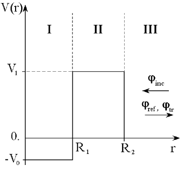
Fig. 3: A spherically symmetric rectangular barrier

Let’s consider the problem of scattering of a particle on the spherically symmetric field, the radial part of which looks like (see Fig. 3):

$$V(r)=\left\{\begin{array}[]{rll}-V_{0},&\mbox{for }r<R_{1};&\mbox{(region I)};\\ V_{1},&\mbox{for }R_{1}<r<R_{2},&\mbox{(region II)};\\ 0,&\mbox{for }r>R_{2},&\mbox{(region III)}.\end{array}\right.$$ (26)

We study the case, when the moment $l=0$ and the energy levels lay below than the height of barrier. Let’s consider the standard stationary method of problem solution. Solving the stationary Schrödinger equation in each region, we obtain the general solution of WF:

$$\psi(r,\theta,\varphi)=\frac{\chi(r)}{r}*Y_{lm}(\theta,\varphi),$$ (27)

$$\chi(r)=\left\{\begin{array}[]{lll}A(e^{-ik_{1}r}-e^{ik_{1}r}),&\mbox{for }r<R_{1},&\mbox{(region I)},\\ \alpha e^{\xi r}+\beta e^{-\xi r},&\mbox{for }R_{1}<r<R_{2},&\mbox{(region II)},\\ e^{-ikr}+Se^{ikr},&\mbox{for }r>R_{2};&\mbox{(region III)},\end{array}\right.$$ (28)

where $Y_{lm}(\theta,\varphi)$ is the spherical function, $k_{1}=\frac{1}{\hbar}\sqrt{2m(E+V_{0})}$, $\xi=\frac{1}{\hbar}\sqrt{2m(V_{1}-E)}$, $k=\frac{1}{\hbar}\sqrt{2mE}$. One can find the unknown coefficients $S$, $A$, $\alpha$ and $\beta$ from the continuity condition for WF and its derivative at points $r=R_{1}$ and $r=R_{2}$. With the stationary point of view the tunneling of particle can be described on the basis of spherical vawes. In the obtained solution it is impossible to separate the vawe transmitted through the barrier from wave reflected from the barrier, and, therefore, to separate their amplitudes (only one item $Se^{ikr}$ contains both transmitted, and reflected waves).

The method of multiple internal reflections allows to find the solution of this problem. Let’s apply it to this problem. We study the propagation of WPs sequentially on steps of its transition in relation to each of boundaries of the barrier (similarly to one-dimensional problem).

In result of multiple internal reflections (and transitions) in relation to the boundaries of the barrier the total time-dependent WF in each region can be written in form of series, composed from the incoming and outcoming WPs. One can calculate the series:

$$\begin{array}[]{lcl}\sum\limits_{n=1}^{+\infty}S^{n}&=&\displaystyle\frac{4ik\xi\biggl{(}\displaystyle\frac{i\xi-k_{1}}{i\xi+k_{1}}-e^{2ik_{1}R_{1}}\biggr{)}e^{-2\xi(R_{2}-R_{1})-2ikR_{2}}}{F_{sub}*(k+i\xi)^{2}},\\ \sum\limits_{n=0}^{+\infty}A^{n}&=&\displaystyle\frac{4ik\xi e^{-ikR_{2}+ik_{1}R_{1}-\xi(R_{2}-R_{1})}}{F_{sub}*(k+i\xi)(k_{1}+i\xi)},\\ \sum\limits_{n=0}^{+\infty}\alpha^{n}&=&\displaystyle\frac{2k\biggl{(}1+\displaystyle\frac{k_{1}-i\xi}{k_{1}+i\xi}e^{2ik_{1}R_{1}}\biggr{)}e^{-(\xi+ik)R_{2}}}{F_{sub}*(k+i\xi)},\\ \sum\limits_{n=0}^{+\infty}\beta^{n}&=&\alpha^{0}*\displaystyle\frac{R_{1}^{-}(1-R_{1}^{+}R_{0}^{-})+T_{1}^{-}R_{0}^{-}T_{1}^{+}}{F_{sub}},\end{array}$$ (29)

where

$$\begin{array}[]{lcl}F_{sub}&=&1+\displaystyle\frac{k_{1}-i\xi}{k_{1}+i\xi}e^{2ik_{1}R_{1}}-\displaystyle\frac{(k-i\xi)(k_{1}-i\xi)}{(k+i\xi)(k_{1}+i\xi)}e^{-2\xi(R_{2}-R_{1})}-\\ &-&\displaystyle\frac{k-i\xi}{k+i\xi}e^{-2\xi(R_{2}-R_{1})+2ik_{1}R_{1}}.\end{array}$$ (30)

Now we determine the incident, transmitted and reflected WPs in relation to the barrier at whole. Considering them for region III, we write:

$$\begin{array}[]{lcl}\chi_{inc}(r,t)&=&\int\limits_{0}^{+\infty}g(E-\bar{E})\theta(V_{1}-E)*e^{-ikr-iEt/\hbar}dE,\\ \chi_{tr}(r,t)&=&\int\limits_{0}^{+\infty}g(E-\bar{E})\theta(V_{1}-E)*S_{tr}*e^{ikr-iEt/\hbar}dE,\\ \chi_{ref}(r,t)&=&\int\limits_{0}^{+\infty}g(E-\bar{E})\theta(V_{1}-E)*S_{ref}e^{ikr-iEt/\hbar}dE,\end{array}$$ (31)

where

$$\begin{array}[]{lcl}S_{tr}&=&\sum\limits_{n=1}^{+\infty}S^{n},\\ S_{ref}&=&S^{0},\\ S&=&S_{tr}+S_{ref}.\end{array}$$ (32)

The expression $S$ represents the S-matrix. Thus, using the method of multiple internal reflections it appears possible to divide it into two components corresponding to amplitudes of transmitted and reflected WPs in relation to the barrier at whole. This property having physical sense, is obtained for the first time.

Expressions for coefficients $S^{n}$, $A^{n}$, $\alpha^{n}$ and $\beta^{n}$ for each step, expression for WF for each step, the series of coefficients $S^{n}$, $A^{n}$, $\alpha^{n}$ and $\beta^{n}$ under the substitution (10) transform into the corresponding expressions for the solution of problem of WP propagation above the barrier. The series of coefficients $S^{n}$, $A^{n}$, $\alpha^{n}$ and $\beta^{n}$ coincide with the corresponding coefficients $S$, $A$, $\alpha$ and $\beta$, calculated by stationary methods.

Similarly to the equations (12) for the one-dimensional problem one can determine the equation for propagation of the maximum of incident, transmitted and reflected WPs in relation to the barrier for the spherically symmetric problem. One can obtain the times necessary for transitting WP through the barrier and for reflecting WP from the barrier:

$$\begin{array}[]{lcl}\tau_{tun}^{Ph}&=&t_{tr}-t_{inc}=\displaystyle\frac{2mR_{2}}{\hbar k}+\hbar\displaystyle\frac{\partial argS_{tr}}{\partial E},\\ \tau_{ref}^{Ph}&=&t_{ref}-t_{inc}=\displaystyle\frac{2mR_{2}}{\hbar k}+\hbar\displaystyle\frac{\partial argS_{ref}}{\partial E}.\end{array}$$ (33)

For the problem of particle tunneling under the barrier we receive:

$$\begin{array}[]{lcl}\tau_{tun}^{Ph}&=&\hbar\displaystyle\frac{\partial}{\partial E}arg\displaystyle\frac{i\xi-k_{1}-(i\xi+k_{1})e^{2ik_{1}R_{1}}}{(i\xi+k)^{2}(i\xi+k_{1})F_{sub}},\\ \tau_{ref}^{Ph}&=&\displaystyle\frac{2m}{\hbar\xi k},\end{array}$$ (34)

and for the problem of WP propagating above the barrier we receive:

$$\begin{array}[]{lcl}\tau_{tun}^{Ph}&=&\displaystyle\frac{2m(R_{2}-R_{1})}{\hbar k_{2}}+\hbar\displaystyle\frac{\partial}{\partial E}arg\displaystyle\frac{k_{2}-k_{1}-(k_{2}+k_{1})e^{2ik_{1}R_{1}}}{(k+k_{2})(k_{1}+k_{2})F_{above}},\\ \tau_{ref}^{Ph}&=&0,\end{array}$$ (35)

where $F_{above}$ can be obtained from the expression for $F_{sub}$ using the substitution (10).

Let’s consider the enough high and wide barrier (limits: $\xi(R_{2}-R_{1})\to\ +\infty$, $\xi\to+\infty$). For tunneling time we obtain the following expression:

$$\tau_{tun}^{Ph}=\displaystyle\frac{2m}{\hbar k\xi}+\displaystyle\frac{4mR_{1}\sin{2k_{1}R_{1}}(1-2\cos{2k_{1}R_{1}})}{\hbar\xi(1-\cos{2k_{1}R_{1}})}.$$ (36)

The tunneling time does not depend on barrier width (the effect of Hartman-Fletcher), but depends on $k_{1}$ and $R_{1}$.

6 Conclusions

At the first time the non-stationary method, describing a process of tunneling of a particle through the barrier on the basis of consideration of multiple internal reflections of wave packets relatively with the barrier boundaries and named as the method of multiple internal reflections, is presented in this paper. In accordence with this method one can describe the tunneling process in dependence on time and study the specific features of tunneling at any interesting moment of time and point of space in details.

The one-dimensional stationary problem of tunneling of the particle through the rectangular barrier with taking into account of the multiple internal reflections was earlier solved [4, 5]. The new specific perspective of the method of multiple internal reflections in solving of this problem is a possibility to fulfill the time analysis of tunneling and reflection in relation to the barrier (with consideration of multiple internal reflections of wave packets).

Using the method of multiple internal reflections the problem of tunneling of a particle through spherically symmetric barrier is considered at the first time and splved. Here, using this method it is possible (as against the known stationary approaches) to separate the wave packet transmitted through the barrier, from the wave packet reflected from the barrier (both packets are spherically divergent). In result, one can calculate such stationary parameters as the coefficient of penetrability of particle through the barrier and the coefficient of reflectivity of particle from the barrier.

In result for the spherically symmetric problem for S-matrix the following property is fulfilled:

$$S=S_{tr}+S_{ref},$$

i. e. it consists of two components corresponding to the transmission and reflection of particle in relation to barrier. This property has physical sense and is justified.

References

• [1] F. Cardone, R. Mignani and V. S. Olkhovsky, About superluminal propagation of an electromagnetic wavepacket inside a rectangular waveguide, Journal de Physique I (France) 7 (10), 1211–1219 (1997).
• [2] V. S. Olkhovsky and E. Recami, Recent developments in the time analysis of tunneling processes, Physics Reports 214 (6), 339–356 (1992).
• [3] V. S. Olkhovsky and A. Agresti in Proc. Adriatico Research Conf. “Tunnelling and its implications” (Trieste, Italy, July 30 - August 2, 1996), D. Mugnai, A. Ranfagni and L. S. Schulman eds. (World Sci., Singapore, 1997), p. 327.
• [4] K. W. McVoy, L. Heller and M. Bolsterli, Reviews of Modern Physics 39, 245 (1967).
• [5] A. Anderson, Multiple scattering approach to one-dimensional potential problems, American Journal of Physics 57 (3), 230–235 (1989).
• [6] M. Razavy and A. Pimpale, Quantum tunneling: a general study in multi-dimensional potential barriers with and without dissipative coupling, Physics Reports 168 (6), 305–370 (1988).
Refer to caption