Exact Analytical Solution of the Constrained Statistical Multifragmentation Model

Abstract

A novel powerful mathematical method is presented, which allows us to find an analytical solution of a simplified version of the statistical multifragmentation model with the restriction that the largest fragment size cannot exceed the finite volume of the system. A complete analysis of the isobaric partition singularities is done for finite system volumes. The finite size effects for large fragments and the role of metastable (unstable) states are discussed.

PACS numbers: 25.70. Pq, 21.65.+f, 24.10. Pa

I Introduction

Exactly solvable models with phase transitions play a special role in the statistical physics - they are the benchmarks of our understanding of critical phenomena that occur in more complicated substances. They are our theoretical laboratories, where we can study the most fundamental problems of critical phenomena which cannot be studied elsewhere. A great deal of progress was recently achieved in our understanding of the multifragmentation phenomenon Bondorf:95 ; Gross:97 ; Moretto:97 when an exact analytical solution of a simplified version of the statistical multifragmentation model (SMM) Gupta:98 ; Gupta:99 was found in Refs. Bugaev:00 ; Bugaev:01 . This exact solution allowed us to elucidate the role of the Fisher exponent $\tau$ on the properties of (tri)critical point and to show explicitly Reuter:01 that in the SMM the relations between $\tau$ and other critical indices differ from the corresponding relations of a well known Fisher droplet model Fisher:64 . Note that these questions in principle cannot be clarified either within the widely used mean-filed approach or numerically.

Despite this success, the application of the exact analytical solution Bugaev:00 ; Bugaev:01 to the description of experimental data is very limited because this solution corresponds to an infinite system volume. To extend the formalism for finite volumes it is necessary to account for the finite size and geometrical shape of the largest fragments, if they are comparable with the system volume. It is clear that these corrections may be important for not too dilute systems. Therefore, to have a more realistic model it is necessary to abandon the arbitrary size of largest fragment and consider the constrained SMM (CSMM) in which the largest fragment size is explicitly related to the volume $V$ of the system. This will allow us to solve the CSMM analytically at finite volumes, to consider how the first order phase transition develops from the singularities of the isobaric partition Goren:81 in thermodynamic limit, and to study the finite size effects for large fragments.

II Laplace-Fourier Transformation

The system states in the SMM are specified by the multiplicity sets $\{n_{k}\}$ ($n_{k}=0,1,2,...$) of $k$-nucleon fragments. The partition function of a single fragment with $k$ nucleons is Bondorf:95 : $V\phi_{k}(T)=V\left(mTk/2\pi\right)^{3/2}~{}z_{k}~{}$, where $k=1,2,...,A$ ($A$ is the total number of nucleons in the system), $V$ and $T$ are, respectively, the volume and the temperature of the system, $m$ is the nucleon mass. The first two factors on the right hand side (r.h.s.) of the single fragment partition originate from the non-relativistic thermal motion and the last factor, $z_{k}$, represents the intrinsic partition function of the $k$- nucleon fragment. Therefore, the function $\phi_{k}(T)$ is a phase space density of the k-nucleon fragment. For $k=1$ (nucleon) we take $z_{1}=4$ (4 internal spin-isospin states) and for fragments with $k>1$ we use the expression motivated by the liquid drop model (see details in Ref. Bondorf:95 ): $z_{k}=\exp(-f_{k}/T),$ with fragment free energy

$$f_{k}=-W(T)~{}k+\sigma(T)~{}k^{2/3}+(\tau+3/2)T\ln k~{},$$ (1)

with $W(T)=W_{\rm o}+T^{2}/\epsilon_{\rm o}$. Here $W_{\rm o}=16$ MeV is the bulk binding energy per nucleon. $T^{2}/\epsilon_{\rm o}$ is the contribution of the excited states taken in the Fermi-gas approximation ($\epsilon_{\rm o}=16$ MeV). $\sigma(T)$ is the temperature dependent surface tension parameterized in the following relation: $\sigma(T)=\sigma_{\rm o}[(T_{c}^{2}~{}-~{}T^{2})/(T_{c}^{2}~{}+~{}T^{2})]^{5/4},$ with $\sigma_{\rm o}=18$ MeV and $T_{c}=18$ MeV ($\sigma=0$ at $T\geq T_{c}$). The last contribution in Eq. (1) involves the famous Fisher’s term with dimensionless parameter $\tau$.

The canonical partition function (CPF) of nuclear fragments in the SMM has the following form:

$$Z^{id}_{A}(V,T)=\sum_{\{n_{k}\}}\left[\prod_{k=1}^{A}\frac{\left[V~{}\phi_{k}(T)\right]^{n_{k}}}{n_{k}!}\right]{\textstyle\delta(A-\sum_{k}kn_{k})}\,.$$ (2)

In Eq. (2) the nuclear fragments are treated as point-like objects. However, these fragments have non-zero proper volumes and they should not overlap in the coordinate space. In the excluded volume (Van der Waals) approximation this is achieved by substituting the total volume $V$ in Eq. (2) by the free (available) volume $V_{f}\equiv V-b\sum_{k}kn_{k}$, where $b=1/\rho_{{\rm o}}$ ($\rho_{{\rm o}}=0.16$ fm^-3 is the normal nuclear density). Therefore, the corrected CPF becomes: $Z_{A}(V,T)=Z^{id}_{A}(V-bA,T)$. The SMM defined by Eq. (2) was studied numerically in Refs. Gupta:98 ; Gupta:99 . This is a simplified version of the SMM, e.g. the symmetry and Coulomb contributions are neglected. However, its investigation appears to be of principal importance for studies of the liquid-gas phase transition.

The calculation of $Z_{A}(V,T)$ is difficult because of the constraint $\sum_{k}kn_{k}=A$. This difficulty can be partly avoided by calculating the grand canonical partition function:

$${\cal Z}(V,T,\mu)~{}\equiv~{}\sum_{A=0}^{\infty}\exp\left({\textstyle\frac{\mu A}{T}}\right)Z_{A}(V,T)~{}\Theta(V-bA)~{},$$ (3)

where $\mu$ denotes a chemical potential. The calculation of ${\cal Z}$ is still rather difficult. The summation over $\{n_{k}\}$ sets in $Z_{A}$ cannot be performed analytically because of additional $A$-dependence in the free volume $V_{f}$ and the restriction $V_{f}>0$. This problem was resolved Bugaev:00 ; Bugaev:01 by the Laplace transformation method to the so-called isobaric ensemble Goren:81 .

In this work we would like to consider a more strict constraint $\sum\limits_{k}^{\alpha V/b}k~{}n_{k}=A$, where the size of the largest fragment cannot exceed the total volume of the system (the parameter $\alpha$ is introduced for convenience). A similar restriction should be also applied to the upper limit of the product in all partitions $Z_{A}^{id}(V,T)$, $Z_{A}(V,T)$ and ${\cal Z}(V,T,\mu)$ introduced above (how to deal with the real values of $\alpha V/b$, see later). Then the model with this constraint, the CSMM, cannot be solved by the Laplace transform method, because the volume integrals cannot be evaluated due to a complicated functional $V$-dependence. However, the CSMM can be solved analytically with the help of the following identity

$$G(V)=\int\limits_{-\infty}^{+\infty}d\xi~{}\int\limits_{-\infty}^{+\infty}\frac{d\eta}{\sqrt{2\pi}}~{}{\textstyle e^{i\eta(V-\xi)}}~{}G(\xi)\,,$$ (4)

which is based on the Fourier representation of the Dirac $\delta$-function. The representation (4) allows us to decouple the additional volume dependence and reduce it to the exponential one, which can be dealt by the usual Laplace transformation. Indeed, with the help of (4) the Laplace transform of the CSMM grand canonical partition (GCP) (3) can be done analytically:

$$\hat{\cal Z}(\lambda,T,\mu)~{}\equiv~{}\int_{0}^{\infty}dV~{}{\textstyle e^{-\lambda V}}~{}{\cal Z}(V,T,\mu)=$$

$$\int_{0}^{\infty}dV^{\prime}\int\limits_{-\infty}^{+\infty}d\xi~{}\int\limits_{-\infty}^{+\infty}\frac{d\eta}{\sqrt{2\pi}}~{}{\textstyle e^{i\eta(V^{\prime}-\xi)-\lambda V^{\prime}}}\times$$

$$\sum_{\{n_{k}\}}\left[\prod_{k=1}^{\alpha\xi/b}~{}\frac{1}{n_{k}!}~{}\left\{V^{\prime}~{}{\textstyle\phi_{k}(T)\,e^{\frac{(\mu-(\lambda-i\eta)bT)k}{T}}}\right\}^{n_{k}}\right]\Theta(V^{\prime})=$$

$$\int_{0}^{\infty}dV^{\prime}\int\limits_{-\infty}^{+\infty}d\xi~{}\int\limits_{-\infty}^{+\infty}\frac{d\eta}{\sqrt{2\pi}}~{}{\textstyle e^{i\eta(V^{\prime}-\xi)-\lambda V^{\prime}+V^{\prime}{\cal F}(\xi,\lambda-i\eta)}}\,.$$ (5)

After changing the integration variable $V\rightarrow V^{\prime}=V-b\sum\limits_{k}^{\alpha\xi/b}k~{}n_{k}$, the constraint of $\Theta$-function has disappeared. Then all $n_{k}$ were summed independently leading to the exponential function. Now the integration over $V^{\prime}$ in Eq. (II) can be straightforwardly done resulting in

$$\hat{\cal Z}(\lambda,T,\mu)=\int\limits_{-\infty}^{+\infty}d\xi\int\limits_{-\infty}^{+\infty}\frac{d\eta}{\sqrt{2\pi}}~{}\frac{\textstyle e^{-i\eta\xi}}{{\textstyle\lambda-i\eta~{}-~{}{\cal F}(\xi,\lambda-i\eta)}}~{},$$ (6)

where the function ${\cal F}(\xi,\tilde{\lambda})$ is defined as follows

$${\cal F}(\xi,\tilde{\lambda})=\sum\limits_{k=1}^{\alpha\xi/b}\phi_{k}(T)~{}e^{\frac{(\mu-\tilde{\lambda}bT)k}{T}}=$$

$$\left(\frac{mT}{2\pi}\right)^{\frac{3}{2}}\left[z_{1}~{}{\textstyle e^{\frac{\mu-\tilde{\lambda}bT}{T}}}+\sum_{k=2}^{\alpha\xi/b}k^{-\tau}e^{\frac{(\mu+W-\tilde{\lambda}bT)k-\sigma k^{2/3}}{T}}\right]\,.\,$$ (7)

As usual, in order to find the GCP by the inverse Laplace transformation, it is necessary to study the structure of singularities of the isobaric partition (II).

III Isobaric Partition Singularities

The isobaric partition (II) of the CSMM is, of course, more complicated than its SMM analog Bugaev:00 ; Bugaev:01 because for finite volumes the structure of singularities in the CSMM is much richer than in the SMM, and they match in the limit $V\rightarrow\infty$ only. To see this let us first make the inverse Laplace transform:

$${\cal Z}(V,T,\mu)~{}=\int\limits_{\chi-i\infty}^{\chi+i\infty}\frac{d\lambda}{2\pi i}~{}\hat{\cal Z}(\lambda,T,\mu)~{}e^{\textstyle\lambda\,V}=$$

$$\int\limits_{-\infty}^{+\infty}d\xi\int\limits_{-\infty}^{+\infty}\frac{d\eta}{\sqrt{2\pi}}\int\limits_{\chi-i\infty}^{\chi+i\infty}\frac{d\lambda}{2\pi i}~{}\frac{\textstyle e^{\lambda\,V-i\eta\xi}}{{\textstyle\lambda-i\eta~{}-~{}{\cal F}(\xi,\lambda-i\eta)}}~{}=$$

$$\int\limits_{-\infty}^{+\infty}d\xi\int\limits_{-\infty}^{+\infty}\frac{d\eta}{\sqrt{2\pi}}\,{\textstyle e^{i\eta(V-\xi)}}\sum_{\{\lambda^{*}_{n}\}}e^{\textstyle\lambda^{*}_{n}\,V}\left[1-\frac{\partial{\cal F}(\xi,\lambda^{*}_{n})}{\partial\lambda^{*}_{n}}\right]^{-1},$$ (8)

where the contour $\lambda$-integral is reduced to the sum over the residues of all singular points $\lambda=\lambda^{*}_{n}+i\eta$ with $n=1,2,..$, since this contour in complex $\lambda$-plane obeys the inequality $\chi>\max(Re\{\lambda^{*}_{n}\})$. Now both remaining integrations in (III) can be done, and the GCP becomes

$${\cal Z}(V,T,\mu)~{}=\sum_{\{\lambda^{*}_{n}\}}e^{\textstyle\lambda^{*}_{n}\,V}\left[1-\frac{\partial{\cal F}(V,\lambda^{*}_{n})}{\partial\lambda^{*}_{n}}\right]^{-1}\,,$$ (9)

i.e. the double integral in (III) simply reduces to the substitution $\xi\rightarrow V$ in the sum over singularities. This is a remarkable result which can be formulated as the following theorem: if the Laplace-Fourier image of the excluded volume GCP exists, then for any additional $V$-dependence of ${\cal F}(V,\lambda^{*}_{n})$ or $\phi_{k}(T)$ the GCP can be identically represented by Eq. (9).

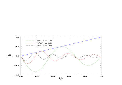
Figure 1: A graphical solution of Eq. (12) for $T=10$ MeV and $\tau=1.825$. The l.h.s. (straight line) and r.h.s. of Eq. (12) (all dashed curves) are shown as the function of dimensionless parameter $I_{2}\,b$ for the three values of the largest fragment size $\alpha V/b$. The intersection point at $(0;\,0)$ corresponds to a real root of Eq. (10). Each tangent point with the straight line generates two complex roots of (10).

The simple poles in (III) are defined by the equation

$$\lambda^{*}_{n}~{}=~{}{\cal F}(V,\lambda^{*}_{n})\,.$$ (10)

In contrast to the usual SMM Bugaev:00 ; Bugaev:01 the singularities $\lambda^{*}_{n}$ are (i) functions of volume $V$, and (ii) they can have a non-zero imaginary part, but in this case there exist pairs of complex conjugate roots of (10) because the GCP is real.

Introducing the real $R_{n}$ and imaginary $I_{n}$ parts of $\lambda^{*}_{n}=R_{n}+iI_{n}$, we can rewrite Eq. (10) as a system of coupled transcendental equations ($K_{up}=\alpha V/b$)

$$R_{n}=~{}\sum\limits_{k=1}^{K_{up}}\tilde{\phi}_{k}(T)~{}{\textstyle e^{\frac{Re(\nu)\,k}{T}}}\cos(I_{n}bk)\,,$$ (11)

$$I_{n}=-\sum\limits_{k=1}^{K_{up}}\tilde{\phi}_{k}(T)~{}{\textstyle e^{\frac{Re(\nu)\,k}{T}}}\sin(I_{n}bk)\,,$$ (12)

where we have introduced the effective chemical potential $\nu=\mu+W(T)-\lambda^{*}_{n}b\,T$, and the reduced distributions $\tilde{\phi}_{1}(T)=z_{1}\exp(-W(T)/T)$ and $\tilde{\phi}_{k>1}(T)=k^{-\tau}\,\exp(-\sigma(T)~{}k^{2/3}/T)$ for convenience.

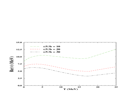
Figure 2: Each curve separates the $T-Re(\nu)$ region of one real root of Eq. (10) (below the curve), three complex roots (on the curve) and five and more roots (above the curve) for three values of $\alpha V/b$ and the same parameters as in Fig. 1.

Consider the real root $(R_{1}>0,I_{1}=0)$, first. For $I_{n}=I_{1}=0$ the real root $R_{1}$ exists for any $T$ and $\mu$. Since for $I_{n}\neq 0$ defined by (12) the inequality $\cos(I_{n}bk)\leq 1$ cannot become the equality for all values of $k$ simultaneously, then from Eq. (11) one obtains

$$R_{n}<\sum\limits_{k=1}^{K_{up}}\tilde{\phi}_{k}(T)~{}{\textstyle e^{\frac{Re(\nu)\,k}{T}}}\quad\Rightarrow\quad R_{n}<R_{1}\,,$$ (13)

where the second inequality (13) immediately follows from the first one. Note that the second inequality (13) plays a decisive role in the thermodynamic limit $V\rightarrow\infty$ because in this case it generates the pressure of the gaseous phase.

Like in the usual SMM Bugaev:00 ; Bugaev:01 , for infinite volume the effective chemical potential must be real and non-positive, $\nu\leq 0$, because in the latter case the function ${\cal F}(V,\lambda_{1}^{*})$ (II) diverges and the formal manipulations in (II) to establish (6) cannot be used. The limiting value $\nu=0$ defines the liquid phase singularity of the isobaric partition which gives the liquid pressure $p_{l}(T,\mu)=R_{1}T=(\mu+W(T))/b$ Bugaev:00 ; Bugaev:01 . But for finite volumes and finite $K_{up}$ the effective chemical potential can be complex (with either sign for its real part) and its value defines the number and position of the imaginary roots $\{\lambda^{*}_{n>1}\}$ in the complex plane. Consider the natural values of $K_{up}$, first. As it is seen from Fig. 1., the r.h.s. of (12) is the amplitude and frequency modulated sine-like function of dimensionless parameter $I_{n}\,b$. Therefore, depending on $T$ and $Re(\nu)$ values there may exist either zero, or finite or infinite number of complex roots $\{\lambda^{*}_{n>1}\}$. In Fig. 1. we showed a special case which corresponds to exactly three roots of Eq. (10) for each value of $K_{up}$: the real root ($I_{1}=0$) and two complex conjugate roots ($\pm I_{2}$). Since the r.h.s. of (12) is monotonously increasing function of $Re(\nu)$, when the former is positive, then it is possible to map the $T-Re(\nu)$ plane into regions of a fixed number of roots of Eq. (10). Each curve in Fig. 2. divides the $T-Re(\nu)$ plane into three parts: for $Re(\nu)$-values below the curve there is only a real root, for points on the curve there exist three roots, and above the curve there are five and more roots of Eq. (10).

A similar situation occurs for the real values of $K_{up}$. In this case all sums in Eqs. (10-13) should be expressed via the Euler-MacLaurin formula

$$\sum\limits_{k=1}^{K_{up}}f_{k}=f(1)+\int\limits_{2}^{K_{up}}dk\,f(k)+{\textstyle\frac{f(K_{up})+f(2)}{2}+\Delta_{f}(K_{up})-}\,$$

$$\Delta_{f}(2)\,,{\rm where}\quad\Delta_{f}(K)=\sum\limits_{n=1}\frac{B_{2n}}{(2n)!}~{}\frac{d^{2n}f(x)}{d\,x^{2n}}\biggr{|}_{x=K}\,.$$ (14)

Here $B_{2n}$ are the Bernoulli numbers. The representation (III) allows one to study the effect of finite volume (FV) on the GCP (9).

IV Finite Volume Thermodynamics

In the CSMM there are two different ways of how the finite volume affects thermodynamical functions: for finite $V$ and $Re(\nu)$ there is always a finite number of simple poles in (9) and all of them contribute into thermodynamic quantities; also the parameter $\alpha<1$ describes a difference between the geometrical shape of the volume under consideration and that one of the largest fragment (assumed to be spherical). To see this, let us study the mechanical pressure which corresponds to the GCP (9)

$$p=T\frac{\partial\ln{\cal Z}(V,T,\mu)}{\partial V}={\textstyle\frac{T}{{\cal Z}(V,T,\mu)}}\sum\limits_{\{\lambda^{*}_{n}\}}\Biggl{[}\frac{\lambda^{*}_{n}~{}e^{\lambda^{*}_{n}\,V}}{1-\frac{\partial{\cal F}(V,\lambda^{*}_{n})}{\partial\lambda^{*}_{n}}}+$$

$$\frac{e^{\lambda^{*}_{n}\,V}}{\left[1-\frac{\partial{\cal F}(V,\lambda^{*}_{n})}{\partial\lambda^{*}_{n}}\right]^{2}}\Biggl{\{}b^{2}\,\frac{\partial\lambda^{*}_{n}}{\partial V}\sum\limits_{k=1}^{K_{up}}\tilde{\phi}_{k}(T)\,k^{2}~{}{\textstyle e^{\frac{\nu\,k}{T}}}+\tilde{\phi}_{K_{up}}(T)\times$$

$${\textstyle e^{\frac{\nu\,K_{up}}{T}}}{\textstyle K_{up}\left[(1-\alpha)+\frac{\nu}{T}\left(\frac{1}{2}-\alpha\right)\right]}+o(K_{up})\Biggr{\}}\Biggr{]}\,,$$ (15)

where we give the main term for $\lambda^{*}_{0}$ and leading FV corrections explicitly for $Re(\nu)/T<1$, whereas $o(K_{up})$ accumulates the higher order corrections due to the Euler-MacLaurin Eq. (III). In evaluation of (IV) we used an explicit representation of the derivative $\partial\lambda^{*}_{n}/\partial V$ which can be found from Eqs. (10) and (III). The first term in the r.h.s. of (IV) describes the partial pressure generated by the simple pole $\lambda^{*}_{n}$ weighted with the “probability” $e^{\lambda^{*}_{n}\,V}/{\cal Z}(V,T,\mu)$, whereas the second and third terms appear due to the volume dependence of $K_{up}$. Note that, instead of the FV corrections, the usage of natural values for $K_{up}(V)$ would generate the artificial delta-function terms in (IV) for the volume derivatives.

As one can see from (IV) for finite volumes the corrections can give a non-negligible contribution to the pressure because in this case $Re(\nu)>0$ can be positive. The real parts of the partial pressures $T\lambda^{*}_{n}$ may have either sign. Therefore, according (13) the positive pressures $TR_{n}>0$ are metastable and the negative ones $TR_{n}<0$ are mechanically unstable. The pair of complex conjugate roots with the same value of $TR_{n}$ corresponds to a formation and decay of those states in thermodynamical system at finite volumes.

When $V$ increases the number of simple poles in (III) also increases and imaginary part of the closest to the real $\lambda$-axis poles becomes very small. For infinite volume the infinite number of simple poles moves toward the real $\lambda$-axis to the vicinity of liquid phase singularity $p_{l}(T,\mu)/T$ and, thus, generates an essential singularity of function ${\cal F}(V,p_{l}/T)$ in (II). In this case the contribution of any of remote poles from the real $\lambda$-axis to the GCP vanishes. Then it can be shown that the FV corrections in (IV) become negligible because of the inequality $Re(\nu)\leq 0$, and, consequently, the reduced distribution of largest fragment $\tilde{\phi}_{K_{up}}(T)=K_{up}^{-\tau}\,\exp(-\sigma(T)~{}K_{up}^{2/3}/T)$ and the derivative $\partial\lambda^{*}_{n}/\partial V$ vanish for all $T$-values, and we obtain the usual SMM solution Bugaev:00 ; Bugaev:01 , and its thermodynamics is governed by the farthest right singularity in complex $\lambda$-plane. The corrections of a similar kind should appear in the entropy, particle number and energy density because of the $T$ and $\mu$ dependence of $\lambda^{*}_{n}$ due to (10) Bugaev:04 . Therefore, these corrections should be taking into account while analyzing the experimental yields of fragments. Then the phase diagram of the nuclear liquid-gas phase transition can be recovered from the experiments on finite systems (nuclei) with more confidence.

Also it is possible that the metastable and unstable modes can emerge in the dynamically expanding system created in experiments, or even there may exist a direct relation between these modes and the spinodal instabilities discussed with respect to phase transition in finite systems Randrup:04 , but it is theme of the other work.

Acknowledgments. This work was supported by the US Department of Energy. The fruitful discussions with Y. H. Chung and M. I. Gorenstein are appreciated.

References

• (1) J. P. Bondorf et al., Phys. Rep. 257 (1995) 131.
• (2) D. H. E. Gross, Phys. Rep. 279 (1997) 119.
• (3) L. G. Moretto et. al., Phys. Rep. 287 (1997) 249.
• (4) S. Das Gupta and A.Z. Mekjian, Phys. Rev. C 57 (1998) 1361.
• (5) S. Das Gupta, A. Majumder, S. Pratt and A. Mekjian, arXiv:nucl-th/9903007 (1999).
• (6) K. A. Bugaev et. al., Phys. Rev. C62 (2000) 044320; arXiv:nucl-th/0007062 (2000).
• (7) K. A. Bugaev et. al., Phys. Lett. B 498 (2001) 144; arXiv:nucl-th/0103075 (2001).
• (8) P.Β T.Β Reuter and K.Β A.Β Bugaev, Phys.Β Lett.Β B 517 (2001) 233.
• (9) M. E. Fisher, Physics 3 (1967) 255.
• (10) M. I. Gorenstein, V. K. Petrov and G. M. Zinovjev, Phys. Lett. B 106 (1981) 327.
• (11) see also K.Β A.Β Bugaev et. al., arXiv:nucl-th/0406034.
• (12) P. Chomaz, M. Colonna, J. Randrup, Phys. Rep. 389 (2004) 263.