Baryon Spectroscopy in Lattice QCD

Abstract

We review recent developments in the study of excited baryon spectroscopy in lattice QCD. After introducing the basic methods used to extract masses from correlation functions, we discuss various interpolating fields and lattice actions commonly used in the literature. We present a survey of results of recent calculations of excited baryons in quenched QCD, and outline possible future directions in the study of baryon spectra.

ADP-04-10/T592
JLAB-THY-04-223
DESY-04-078

1 Introduction and Motivation

One of the primary tools used for studying the forces which confine quarks inside hadrons, and determining the relevant effective degrees of freedom in strongly coupled QCD, has been baryon and meson spectroscopy. This is a driving force behind the current experimental $N^{*}$ programme at Jefferson Lab, which is accumulating data of unprecedented quality and quantity on various $N\to N^{*}$ transitions CLAS . The prospects of studying mesonic spectra, and in particular the role played by gluonic excitations, has been a major motivation for future facilities such as CLEO-c CLEOC , the anti-proton facility at GSI (PANDA) PANDA , and the Hall D programme at a 12 GeV energy upgraded CEBAF HALLD . With the increased precision of the new $N^{*}$ data comes a growing need to understand the observed spectrum within QCD. QCD-inspired phenomenological models, whilst successful in describing many features of the $N^{*}$ spectrum CR , leave many questions unanswered.

One of the long-standing puzzles in baryon spectroscopy has been the low mass of the first positive parity excitation of the nucleon, the $N^{*}(1440)$ Roper resonance, compared with the lowest lying odd parity excitation. In valence quark models with harmonic oscillator potentials, the $J^{P}={1\over 2}^{-}$ state naturally occurs below the $N=2$, ${1\over 2}^{+}$ excitation IK . Without fine tuning of parameters, valence quark models tend to leave the Roper mass too high. Similar difficulties in the level orderings appear for the $J^{P}={3\over 2}^{+}$ $\Delta^{*}(1600)$ and ${1\over 2}^{+}$ $\Sigma^{*}(1690)$ resonances, which have led to speculations that the Roper resonances may be more appropriately viewed as hybrid baryon states with explicitly excited glue field configurations LBL , rather than as radial excitations of a three-quark configuration. Other scenarios portray the Roper resonances as “breathing modes” of the ground states BREATHE , or states which can be described in terms of meson-baryon dynamics alone FZJ .

Another challenge for spectroscopy is presented by the anomalously small mass of the odd parity $\Lambda(1405)$ hyperon. This is alternatively interpreted as a true three-quark state, or as a hadronic molecule arising from strong coupled channel effects between $\Sigma\pi$, $\bar{K}N$, $\ldots$ states L1405 . In fact, the role played by Goldstone bosons in baryon spectroscopy has received considerable attention recently MASSEXTR ; YOUNG ; Morel:2003fj .

Mass splittings between states within SU(3) quark-model multiplets provide another important motivation for studying the baryon spectrum. The dynamical origin of hyperfine splittings in quark models has traditionally been attributed to the colour-magnetic one gluon exchange mechanism RUJ . On the other hand, there have been attempts recently to explain the hyperfine splittings and level orderings in terms of a spin-flavour interaction associated with the exchange of a pseudoscalar nonet of Goldstone bosons between quarks GBE . Understanding the mass splitting between the $J^{P}={1\over 2}^{-}$ $N^{*}(1535)$ and ${3\over 2}^{-}$ $N^{*}(1520)$, or between the ${1\over 2}^{-}$ $\Delta^{*}(1620)$ and ${3\over 2}^{-}$ $\Delta^{*}(1700)$, can help identify the important mechanisms associated with the hyperfine interactions, and shed light on the spin-orbit force, which has been a central mystery in spectroscopy SUMRULES . In valence quark models, the degeneracy between the $N{1\over 2}^{-}$ and $N{3\over 2}^{-}$ can be broken by a tensor force associated with mixing between the $N^{2}$ and $N^{4}$ representations of SU(3) CR , although this generally leaves the $N{3\over 2}^{-}$ at a higher energy than the $N{1\over 2}^{-}$. In contrast, a spin-orbit force is necessary to split the $\Delta{3\over 2}^{-}$ and $\Delta{1\over 2}^{-}$ states. In the Goldstone boson exchange model GBE , both of these pairs of states are degenerate.

Similarly, neither spin-flavour nor colour-magnetic interactions is able to account for the mass splitting between the $\Lambda(1405)$ and the $J^{P}={3\over 2}^{-}$ $\Lambda^{*}(1520)$. A splitting between these can arise in constituent quark models with a spin-orbit interaction, but the required strength of the interaction leads to spurious mass splittings elsewhere CR ; CI . In fact, model-independent analyses of baryons in the large $N_{c}$ limit LARGE_NC have found that these mass splittings receive important contributions from operators that do not have a simple quark model interpretation LARGE_NC , such as those simultaneously coupling spin, isospin and orbital angular momentum, as anticipated by early QCD sum-rule analyses SUMRULES . Of course, the coefficients of the various operators in such an analysis must be determined phenomenologically and guidance from lattice QCD is essential.

The large number of “missing” resonances, predicted by the constituent quark model and its generalisations but not observed experimentally, presents another problem for spectroscopy. If these states do not exist, this may suggest that perhaps a quark–diquark picture (with fewer degrees of freedom) could afford a more efficient description. Alternatively, the missing states could simply have weak couplings to the $\pi N$ system CR .

Apart from these long-standing puzzles, interest in baryon spectroscopy has been further stimulated with the recent discovery of the exotic strangeness $S=+1$ $\Theta^{+}$ pentaquark 5Q , which has a minimum 5 valence quark ($uudd\bar{s}$) content. Postulated long ago, the $\Theta^{+}$ appears to have eluded searches until now, and understanding its properties and internal structure has become a major challenge for spectroscopy.

A consistent description of the baryon spectrum within low-energy models requires a satisfactory resolution of the old questions of spectroscopy, as well as insight into the new puzzles. On both of these fronts real progress may only come with the help of first-principle calculations of the spectrum in lattice QCD, which at present is the only method capable of determining hadron properties directly from the fundamental quark and gluon theory. Considerable progress has been made in the past few years in calculating hadronic properties in both quenched and full QCD, with the ground state masses now understood at the few percent level.

Compared with simulations of hadron ground state properties, however, the calculation of the excited nucleon spectrum places particularly heavy demands on lattice spectroscopy. The excited nucleon states are expected to be large, with the size of a state expected to double with each increase in orbital angular momentum. Lattice studies of the excited nucleon spectrum therefore require large lattice volumes, with correspondingly large computational resources. Furthermore, the states are relatively massive, requiring a fine lattice spacing, at least in the temporal direction. Recent advances in computational capabilities and more efficient algorithms have enabled the first dedicated lattice QCD simulations of the excited states of the nucleon to be undertaken.

Of course, the calculation of the hadronic spectrum faces a formidable challenge in describing excited state decays, which is relevant in both full and quenched QCD. Lattice studies of excited hadrons are possible because at the current unphysically large quark masses and finite volumes used in the simulations many excited states are stable RHO . Contact with experiment can be made via extrapolations incorporating the nonanalytic behaviour predicted by chiral effective field theory.

The rest of this review is laid out as follows. After briefly reviewing in Section 2 the history of lattice calculations of the excited baryon spectrum, in Section 3 we outline the basic lattice techniques for extracting masses from correlation functions, including variational methods and Bayesian statistics. Section 4 describes the construction of a suitable basis of interpolating fields for any baryon we may wish to investigate. Section 5 outlines the simplest interpolating fields for spin-1/2 and spin-3/2 baryons, and how these can be used in the construction of lattice correlation functions. In Section 6, we present a survey of recent $N^{*}$ results for both positive and negative parity baryons. Finally, in Sec. 7 we discuss conclusions of the existing studies, and speculate on future directions for the study of baryon spectra. Some technical aspects of the correlation matrix formalism for calculating masses, coupling strengths and optimal interpolating fields are described in the Appendix.

2 History of Lattice $N^{*}$ Calculations

The history of excited baryons on the lattice is rather short, although recently there has been growing interest in finding new techniques to isolate excited baryons, motivated partly by the experimental $N^{*}$ programme at Jefferson Lab. An attempt to determine the first positive-parity excitation of the nucleon using variational methods was made by the UKQCD collaborationukqcd93 . A more detailed analysis of the positive parity excitation of the nucleon was performed by Leinweber DEREK using Wilson fermions and an operator product expansion spectral ansatz. DeGrand and Hecht DEGRAND92 used a wave function ansatz to access $P$-wave baryons, with Wilson fermions and relatively heavy quarks. Subsequently, Lee and Leinweber LL introduced a parity projection technique to study the negative parity ${1\over 2}^{-}$ states using an ${\cal O}(a^{2})$ tree-level tadpole-improved D_χ34 quark action, and an ${\cal O}(a^{2})$ tree-level tadpole-improved gauge action. Following this, Lee LEE reported results using a D₂₃₄ quark action with an improved gauge action on an anisotropic lattice to study the ${1\over 2}^{+}$ and ${1\over 2}^{-}$ excitations of the nucleon. An anisotropic lattice with an ${\cal O}(a)$ improved quark action was also used by Nakajima et al. Nakajima:2001js to study excited states of octet and decuplet baryons.

The RIKEN-BNL group BNL has stressed the importance of maintaining chiral symmetry on the lattice. At finite lattice spacing the Wilson fermion action is known to explicitly break the chiral symmetry of continuum QCD. A solution to this problem is provided through the introduction of a fifth dimension, which allows chiral symmetry to be maintained even at non-zero lattice spacing DWF . The resulting domain wall fermion action was used in Ref. BNL to compute the masses of the $N{1\over 2}^{-}$ and $N{1\over 2}^{+}$ excited states. The analysis has recently been extended by studying the finite volume effects of the first $N{1\over 2}^{+}$ excited state extracted using maximum entropy methods Sasaki:2003xc .

A nonperturbatively ${\cal O}(a)$-improved Sheikholeslami-Wohlert (SW) CLOVER , or clover, fermion action was used by Richards et al. RICHARDS to study the $N{1\over 2}^{-}$ and $\Delta{3\over 2}^{-}$ states. By appropriately choosing the coefficient of the improvement term, all ${\cal O}(a)$ discretisation uncertainties can be removed, ensuring that continuum-like results are obtained at a finite lattice spacing. For more details on ${\cal O}(a)$-improvement, see the contribution by Zanotti et al. in this lecture series.

The BGR collaboration FP has been investigating the masses of the $N{1\over 2}^{-}$ and $N{1\over 2}^{+}$ excited states calculated with chirally improved (CI) and Fixed Point (FP) fermions. Both of these actions offer the advantage of improved chiral properties over traditional Wilson-style fermions, without the cost associated with Ginsparg-Wilson fermions, which possess an exact analogue of chiral symmetry.

The CSSM Lattice Collaboration has used an ${\cal O}(a^{2})$ improved gluon action and the ${\cal O}(a)$-improved Fat Link Irrelevant Clover (FLIC) fermion action FATJAMES to perform a comprehensive study of the spectrum of positive and negative parity baryons CSSM ; CSSM32 . Excited state masses in both the octet and decuplet multiplets have been computed, including the $N{1\over 2}^{\pm}$, $N{3\over 2}^{\pm}$, $\Sigma{1\over 2}^{\pm}$, $\Lambda{1\over 2}^{\pm}$, $\Xi{1\over 2}^{\pm}$, $\Delta{1\over 2}^{\pm}$ and $\Delta{3\over 2}^{\pm}$ baryons. The formulation of FLIC fermions and a review of its scaling and light quark mass phenomenology is reviewed by Zanotti et al. in this lecture series.

Constrained-fitting methods originating from Bayesian priors have also recently been used by Lee et al. BAYESIAN to study the two lowest octet and decuplet positive and negative parity baryons, using overlap fermions with pion masses down to $\sim 180$ MeV. These authors have addressed the difficult issue of contamination of the first excited state of the nucleon with quenched $\eta^{\prime}N$ artifacts Dong:2003zf . While these authors claim to have observed the Roper in quenched QCD, it remains to be demonstrated that this conclusion is independent of the Bayesian-prior assumed in their analysis DEREK . It would be interesting to examine these correlation functions using correlation matrix techniques or alternative Bayesian techniques such as the Maximum Entropy Method.

As mentioned in Sec. 1, we are currently seeing intense interest in exotic pentaquark spectroscopy, and recently the first lattice studies of 5-quark states have appeared 5Q_CSIKOR ; 5Q_SASAKI ; 5Q_CHIU . Here the unique advantage of lattice QCD can come to the fore, in predicting, for instance, the parity and spin of the lowest lying pentaquark state, which are as yet undetermined experimentally. The first two of these early studies have used the standard Wilson gauge and fermion action, on lattice sizes of $L=1.2$–2.7 fm 5Q_CSIKOR , and $L=2.2$ fm 5Q_SASAKI , while the third used domain wall fermions with a Wilson gauge action on a $L=1.8$ fm lattice.

The main challenge here has been the construction of lattice operators for states with 4 quarks and an antiquark, which can be variously constructed in terms of ($qqq$)($q\bar{s}$) “nucleon–meson” 5Q_CSIKOR or ($qq$)($qq$)$\bar{s}$ “diquark-diquark-$\bar{s}$” 5Q_SASAKI ; 5Q_CHIU operators. While two of these studies 5Q_CSIKOR ; 5Q_SASAKI appear to favor negative parity for the lowest lying pentaquark state, it is not clear that this state is a new resonant combination of $K\,N$ in $S$ wave. The most recent study 5Q_CHIU reports an even parity ground state, and moreover identifies the Roper resonance as a pentaquark state. The relatively small volumes, limited set of interpolating fields, and naive linear extrapolations means that these results must be regarded as exploratory at present. New studies using the FLIC fermion action with several different interpolating fields are currently in progress 5Q_FLIC .

We are clearly witnessing an exciting period in which the field of baryon spectroscopy on the lattice is beginning to flourish.

3 Lattice Techniques

3.1 Spectroscopy Recipe

The computation of the spectrum of states in lattice QCD is in principle straightforward. The building blocks are the quark propagators

$$S^{ij}_{\alpha\beta}(x,y)=\langle 0|\psi^{i}_{\alpha}(x)\bar{\psi}^{j}_{\beta}(y)|0\rangle,$$ (1)

computed on an ensemble of gauge configurations, composed of gauge field links $U_{\mu}(x)\simeq\exp\{iagA_{\mu}(x)\}$. The calculation then proceeds as follows:

1. Choose an interpolating operator ${\cal O}$ that has a good overlap with $P$, the state of interest,

   $$\langle 0\mid{\cal O}\mid P\rangle\neq 0,$$

   and ideally a small overlap with other states having the same quantum numbers.

2. Form the time-sliced correlation function

   $$G(t,\vec{p})=\sum_{\vec{x}}\langle{\cal O}(\vec{x},t){\cal O}^{\dagger}(\vec{0},0)\rangle e^{-i\vec{p}\cdot\vec{x}},$$

   which can be expressed by a Wick expansion in terms of the elemental quark propagators of Eq. (1).

3. Insert a complete set of states between ${\cal O}$ and ${\cal O}^{\dagger}$. The time-sliced sum puts the intermediate states at definite momentum, and one finds

   $$G(t,\vec{p}) = \sum_{\vec{x}}\sum_{P}\int\frac{d^{3}k}{(2\pi)^{3}2E(\vec{k})}e^{-i\vec{p}\cdot\vec{x}}\langle 0|{\cal O}(\vec{x},t)|P(\vec{k})\rangle\langle P(\vec{k})|{\cal O}^{\dagger}(\vec{0},0)|0\rangle$$

   $$= \sum_{P}\frac{\mid\langle 0\mid{\cal O}\mid P\rangle\mid^{2}}{2\,E_{P}(\vec{p})}e^{-iE_{P}(\vec{p})t}\ ,$$

   where the sum over $P$ includes the contributions from two-particle and higher states.

4. Continue to Euclidean space $t\rightarrow-it$, giving

   $$G(t,\vec{p})=\sum_{P}\frac{\mid\langle 0\mid{\cal O}\mid P\rangle\mid^{2}}{2\,E_{P}(\vec{p})}e^{-E_{P}(\vec{p})t}.$$ (2)

At large Euclidean times, the lightest state dominates the spectral sum in Eq. (2), and we can extract the ground state mass. The determination of this ground state mass for the states of lowest spin has been the benchmark calculation of lattice QCD since its inception. However, our goal is to build up a more complete description of the baryon spectrum, ultimately determining not only the masses of some of the higher spin particles, but also the masses of the radial excitations. In the remainder of this section, we will address two issues that are crucial to attaining this goal: the application of variational techniques to isolate the higher excitations in Eq. (2), and the use of the appropriate statistical fitting techniques to reliably extract the energies of those excitations. In the following section, we will describe the construction of the nucleon interpolating operators.

3.2 Fitting Techniques

Variational Methods

To confidently extract other than the lowest-lying state in Eq. (2), it is crucial to have more than a single interpolating operator ${\cal O}_{i}$ in order to appeal to variational methods to determine the spectrum of states michael85 ; lw90 . Our aim is to measure every element of the matrix of correlators

$$G_{ij}(t)=\langle\sum_{\vec{x}}{\cal O}_{i}(\vec{x},t){\cal O}^{\dagger}_{j}(0)\rangle.$$ (3)

We now consider the eigenvalue equation

$$G(t)u=\lambda(t,t_{0})G(t_{0})u,$$ (4)

for some eigenfunction $u$ of $G^{-1}(t_{0})G(t)$, with $t_{0}$ fixed. For the sake of illustration, we will consider a simple system with only two independent states, and a $2\times 2$ matrix of correlators. Then the eigenvalues of Eq. (4) satisfy

$$\lambda_{+}(t,t_{0}) = e^{-(t-t_{0})E_{0}}\ ,$$ (5)

$$\lambda_{-}(t,t_{0}) = e^{-(t-t_{0})E_{1}}\ ,$$ (6)

and we have an exact separation between the energies of the two states, with coefficients growing exponentially with $t_{0}$. For the physical case of more than two states, there are exponential corrections arising from the states of higher energy. Ideally, to suppress the contribution of these higher energy states we would wish to choose $t_{0}$ to have as large a value as possible. However, increasing $t_{0}$ comes at the price of increasing statistical noise, and therefore we are generally obliged to take $t_{0}$ close to the origin.

In practice, it is usual to adopt a variation of the above method, and not to attempt to diagonalise the transfer matrix at each time slice, but rather to choose a matrix of eigenvectors $V(t_{0})$ for some $t_{0}$ close to the source that diagonalises $G(t_{0})^{-1}G(t_{0}+1)$ . For the case of a $2\times 2$ matrix with only two states, the diagonal elements of the matrix

$$V(t_{0}+1)^{-1}G(t_{0})^{-1}G(t)V(t_{0}+1)$$

are indeed equivalent to the eigenvalues of $G(t_{0})^{-1}G(t_{0}+1)$. A more pedagogical discussion of these concepts can be found in the Appendix.

The efficacy of this method relies on having a basis of correlators that can delineate the structure of the first few states, together with sufficiently high-quality statistics that the elements of the correlator matrix can be well determined. In the case of the glueball spectrum, the computational cost is dominated by the cost of generating the gauge configurations, and the overhead of measuring extra correlators is negligible. Furthermore, we are able to improve the statistical quality of the data by using translational invariance to average over the position of the source coordinate in Eq. (2). Variational techniques have been essential, and very successful, in the extraction of the glueball spectrum MCNEILE ; Morningstar:1999rf .

In the case of operators containing quark fields, there is generally a considerable computational cost associated with the measurement of additional correlators. We will discuss the construction of such operators in the next section, but it is straightforward to see how this cost arises. Recall that the basic building blocks of spectroscopy are the quark propagators of Eq. (1), which satisfy

$$M^{ij}_{\alpha\beta}(x,y)S^{jk}_{\beta\gamma}(y,z)=\delta^{ik}\delta_{\alpha\gamma}\delta_{xz}.$$ (7)

where $M$ is the fermion matrix of the fermion action $\overline{\psi}\,M\,\psi$. The propagator is usually obtained by standard sparse matrix inversion methods, such as conjugate gradient. These methods are applicable to a fixed source vector on the right hand side of Eq. (7), and additional correlators require the inversion of $M$ for additional source vectors. A corollary of this is that the matrix of correlators is obtained for fixed source coordinate, and therefore we cannot in general use translational invariance to average over the source coordinate in the manner of glueball calculations.

Bayesian Statistics

Given the computational cost of measuring additional correlators, it is important to extract the greatest possible information from the those that are measured. Furthermore, it is vital that the fitting procedure be as reliable as possible, in particular by ensuring that the extracted masses are not adversely affected by contamination from higher excitations. Historically, lattice calculations employed maximum likelyhood fits to correlators such as Eq. (2), using a single or at most two states in the spectral sum. An acceptable $\chi^{2}/{\rm d.o.f.}$ would only be obtained if the fitted data were restricted to large temporal separations, in which one or two states did indeed dominate the spectral sum. Thus the fits ignored the data at small temporal separations, which we have already seen has the largest signal-to-noise ratio.

It is natural to ask whether one can extract useful information from the data at small values of $t$, and a means of so doing is provided through the use of Bayesian Statistics. We will return to a further discussion of the the Bayesian approach in our survey of results.

4 Interpolating Fields

The variational techniques and fitting methods described above require a suitable basis of interpolating fields from which operators can be constructed which mimic the structure of each of the states to be extracted. In order to do so, we firstly have to consider the possible quantum numbers by which states are classified, and the extent to which they remain good quantum numbers in lattice calculations. We then have to consider the spatial structure of the states, and in particular their spatial extents, and whether we can construct interpolating operators that reflect the structure, through the use of, say, smeared interpolating fields. We will begin this section by detailing the quantum numbers with which states are classified, namely flavour and parity, and the degree to which they are good quantum numbers on the lattice. We will then proceed to discuss the use of spatially extended interpolating operators, known as smearing. Finally, we will describe the operators that have been employed thus far in lattice calculations, and discuss these in terms of continuum quark model operators.

4.1 Continuum and Lattice Symmetries

Baryon states are classified by their flavour structure, either according to $SU(2)$ (isospin), or $SU(3)$ (strangeness), parity, and total spin. In nearly all lattice calculations of the hadron spectrum, exact isospin symmetry is imposed so the $m_{u}=m_{d}$, and electromagnetic effects are ignored. Thus the flavour structure of baryon states composed of light ($u,d,s$) quarks is specified according to Total Isospin $I$, $I_{3}$, and the strangeness $S$, and the naming of baryon states follows from this labeling, as detailed in Table 1.

Table 1: The table shows the flavour classification of baryon states constructed from light ($u,d,s$) quarks, together with a representative flavour structure in terms of three valence quarks for the case $I_{3}=I$.

$I$	$S$	Baryon	Flavour structure ($I_{3}=I$)
$1/2$	$0$	$N$	$\frac{1}{\sqrt{2}}(\mid udu\rangle-\mid duu\rangle)$
$3/2$	$0$	$\Delta$	$\mid uuu\rangle$
$0$	$-1$	$\Lambda$	$\frac{1}{\sqrt{2}}(\mid uds\rangle-\mid dus\rangle)$
$1$	$-1$	$\Sigma$	$\mid uus\rangle$
$1/2$	$-2$	$\Xi$	$\mid uss\rangle$
$0$	$-3$	$\Omega$	$\mid sss\rangle$

The flavour structure is straightforward to implement in the calculation of the correlation functions by only including the appropriate contractions in the Wick expansion of Eq. (2).

4.2 Angular Momentum and Lattice QCD

More delicate is the identification of the spin of particles in a lattice calculation. For the discussion of the spectrum, we are principally interested in the study of states at rest, for which the relevant continuum symmetry for classifying states is their properties under rotations, described by the group $SU(2)$. The irreducible representations of $SU(2)$ are labeled by the total spin $J$, and the projection of spin along a particular axis, say $J_{3}$, in the manner of isospin. We have already seen that we can impose exact isospin symmetry in our calculations, but the use of a hypercubic lattice has the consequence that we no longer have exact three-dimensional rotational symmetry, but rather the symmetries of the three-dimensional cubic group of the three-dimensional spatial lattice, the octahedral group ${\cal O}$ elliott .

In contrast to the continuum rotation group, ${\cal O}$ is a finite group. It contains a total of 48 elements, and has a total of five single-valued irreducible representations (IR), corresponding to states of integer spin, and only three double-valued IRs, corresponding to states of half-integer spin. Thus each lattice IR is an admixture of different values of $J$, listed for the double-valued representations in Table 2 johnson82 .

Table 2: Irreducible representations of the octahedral group, listing the number of elements and the spin content.

Representation	Dimension	Spin ($J$)
$G_{1}$	2	$1/2,7/2,9/2,\dots$
$G_{2}$	2	$5/2,7/2,11/2,\dots$
$H$	4	$3/2,5/2,7/2,\dots$

Thus in any lattice calculation at a fixed value of the lattice spacing, we will aim to construct operators transforming irreducibly according to one of the IRs of Table 2, and extract the spectrum of states within each of these IRs. We will only be able to identify the angular momentum of the various states when we look for commonality between the masses extracted from the various IRs in the approach to the continuum limit. Thus, for example, the continuum state of spin $5/2$ has two degrees of freedom associated with $G_{2}$, and the remaining four degrees of freedom associated with $H$.

So far, most lattice calculations have employed local, $S$-wave propagators for the quarks, and as we shall see later, have employed operators transforming according to the IRs $G_{1}$, for spin $\frac{1}{2}$, or $H$, for spin $\frac{3}{2}$, and have implicitly assumed that these states with these spins are indeed the lightest states in their respective representations, as observed in the physical hadron spectrum. The technology required to construct general baryon interpolating operators transforming irreducibly under $O$ has now be developed morningstar03 ; lhpcops03 , and a preliminary attempt at the spectrum using $P$-wave quark propagators has been made in ref. sato03 .

4.3 Parity

The remaining symmetry that we must consider is parity, corresponding to the spatial-inversion operator $I_{s}$. Clearly, this is a good symmetry on our hypercubic lattice, yielding the point group $O_{h}$, with 96 elements, and an additional subscript $g$ or $u$ on our irreducible representations corresponding to positive- and negative-parity representations respectively. One subtlety arises when one considers the determination of the spectrum on a lattice with either periodic or anti-periodic boundary conditions in the temporal direction. In that case, for identical source and sink we have

$$G(t) = \sum_{\vec{x}}\langle{\cal O}_{+}(\vec{x},t)\overline{\cal O}_{+}(0)\rangle$$ (8)

$$\longrightarrow \sum_{P_{+}}|A_{P_{+}}|^{2}e^{-M_{P_{+}}t}\pm\sum_{P_{-}}|A_{P_{-}}|^{2}e^{-M_{P_{-}}(N_{t}-t)}\ ,$$ (9)

where ${\cal O}_{+}$ is an interpolating operator designed to isolate states of positive parity propagating in the forward time direction, $N_{t}$ is the temporal extent of the lattice, $A_{P}$ is the amplitude of a state $P$, and the subscripts $+~{}\mbox{and}~{}-$ denote contributions of states of positive or negative parity respectively. As discussed further in Sec. 5.1, a similar expression may be obtained for the opposite parity states. Thus we see that a complete delineation of the states on a periodic lattice only occurs as $N_{t}\to\infty$. The superposition of results from periodic and anti-periodic boundary conditions can be used to eliminate the second term of Eq. (9). Alternatively, a fixed boundary condition can be used to eliminate the second term of Eq. (9) by preventing states from crossing the temporal boundary of the lattice.

4.4 Smearing and Extended Interpolating Fields

It is common to perform some smearing in the spatial dimensions at the source to increase the overlap of the interpolating operators with the ground states. Here we describe one such technique to do this: gauge-invariant Gaussian smearing Gusken:qx .

The source-smearing technique Gusken:qx starts with a point source,

$$\psi_{0\,\alpha}^{\phantom{0}\,a}({\vec{x}},t)=\delta^{ac}\delta_{\alpha\gamma}\delta_{{\vec{x}},{\vec{x}}_{0}}\delta_{t,t_{0}}$$ (10)

for source colour $c$, Dirac $\gamma$, position ${\vec{x}}_{0}$ and time $t_{0}$, and proceeds via the iterative scheme,

$$\psi_{i}({\vec{x}},t)=\sum_{{\vec{x}}^{\prime}}F({\vec{x}},{\vec{x}}^{\prime})\,\psi_{i-1}({\vec{x}}^{\prime},t)\,,$$

where

$$F({\vec{x}},{\vec{x}}^{\prime})=\frac{1}{(1+\alpha)}\left(\delta_{{\vec{x}},{\vec{x}}^{\prime}}+\frac{\alpha}{6}\sum_{\mu=1}^{3}\left[U_{\mu}({\vec{x}},t)\,\delta_{{\vec{x}}^{\prime},{\vec{x}}+\widehat{\mu}}+U_{\mu}^{\dagger}({\vec{x}}-\widehat{\mu},t)\,\delta_{{\vec{x}}^{\prime},{\vec{x}}-\widehat{\mu}}\right]\right)\,.$$

Repeating the procedure $N$ times gives the resulting fermion source,

$$\psi_{N}({\vec{x}},t)=\sum_{{\vec{x}}^{\prime}}F^{N}({\vec{x}},{\vec{x}}^{\prime})\,\psi_{0}({\vec{x}}^{\prime},t)\,.$$ (11)

The parameters $N$ and $\alpha$ govern the size and shape of the smearing function. The propagator $S$ is obtained from the smeared source by solving

$$M_{\alpha\beta}^{ab}\,S_{\beta\gamma}^{bc}=\psi_{\alpha}^{a}\,,$$ (12)

for each colour, Dirac source $c,\,\gamma$ respectively of Eq. (10) via a standard matrix inverter such as the BiStabilised Conjugate Gradient algorithm BiCG .

5 Operators for Spin-${1\over 2}$ and Spin-${3\over 2}$ Baryons

We will now see how the considerations described above apply to the construction of operators for the spin-${1\over 2}$ and spin-${3\over 2}$ baryons. Initially we will construct the operators based on analogy with the construction of the interpolating operators of the continuum, first for spin ${1\over 2}$ and then for spin ${3\over 2}$. We will then briefly describe the construction of the operators that transform irreducibly under the lattice symmetries directly, without reference to the continuum discussion.

5.1 Spin-${1\over 2}$ Baryons: General Considerations

Following standard notation, we define a two-point correlation function for a spin-$\frac{1}{2}$ baryon $B$ as

$$G_{B}(t,{\vec{p}})\equiv\sum_{\vec{x}}\,e^{-i{\vec{p}}\cdot{\vec{x}}}\left\langle\Omega\left|\chi_{B}(x)\bar{\chi}_{B}(0)\right|\Omega\right\rangle$$ (13)

where $\chi_{B}$ is a baryon interpolating field and where we have suppressed Dirac indices. All formalism for correlation functions and interpolating fields presented in this article is carried out using the Dirac representation of the Dirac $\gamma$-matrices. The choice of interpolating field $\chi_{B}$ is discussed in Section 5.2 below. The overlap of the interpolating field $\chi_{B}$ with positive or negative parity states $|B^{\pm}\rangle$ is parameterised by a coupling strength $\lambda_{B^{\pm}}$ which is complex in general and which is defined by

$$\left\langle\Omega\left|\,\chi_{B}(0)\,\right|B^{+},p,s\right\rangle\!\! = \!\!\lambda_{B^{+}}\sqrt{M_{B^{+}}\over E_{B^{+}}}\ u_{B^{+}}(p,s)\,,$$ (14)

$$\left\langle\Omega\left|\,\chi_{B}(0)\,\right|B^{-},p,s\right\rangle\!\! = \!\!\lambda_{B^{-}}\sqrt{M_{B^{-}}\over E_{B^{-}}}\,\gamma_{5}u_{B^{-}}(p,s)\,,$$ (15)

where $M_{B^{\pm}}$ is the mass of the state $B^{\pm}$, $E_{B^{\pm}}=\sqrt{M_{B^{\pm}}^{2}+{\vec{p}\,}^{2}}$ is its energy, and $u_{B^{\pm}}(p,s)$ is a Dirac spinor with normalisation $\overline{u}_{B^{\pm}}^{\alpha}(p,s)u_{B^{\pm}}^{\beta}(p,s)=\delta^{\alpha\beta}$. For large Euclidean time, the correlation function can be written as a sum of the lowest energy positive and negative parity contributions

$$G_{B}(t,{\vec{p}})\approx\lambda_{B^{+}}^{2}{\left(\gamma\cdot p+M_{B^{+}}\right)\over 2E_{B^{+}}}e^{-E_{B^{+}}\,t}+\lambda_{B^{-}}^{2}{\left(\gamma\cdot p-M_{B^{-}}\right)\over 2E_{B^{-}}}e^{-E_{B^{-}}\,t}\ ,$$ (16)

when a fixed boundary condition in the time direction is used to remove backward propagating states. The positive and negative parity states are isolated by taking the trace of $G_{B}$ with the operator $\Gamma_{+}$ and $\Gamma_{-}$ respectively, where

$$\Gamma_{\pm} = {1\over 2}\left(1\pm{M_{B^{\mp}}\over E_{B^{\mp}}}\gamma_{4}\right)\ .$$ (17)

For $\vec{p}=0$, the energy $E_{B^{\mp}}=M_{B^{\mp}}$, so that $\Gamma_{\mp}^{2}=\Gamma_{\mp}$ and the $\Gamma_{\mp}$ are parity projectors In this case, positive parity states propagate in the (1, 1) and (2, 2) elements of the Dirac $\gamma$-matrix of Eq. (16), while negative parity states propagate in the (3, 3) and (4, 4) elements, and the masses of $B^{\mp}$ may be isolated.

5.2 Spin-${1\over 2}$ Baryons: Interpolating Fields

There are two types of interpolating fields which have commonly been used in the literature. The notation adopted here is similar to that of Ref. LWD . To access the positive parity proton we use as interpolating fields

$$\chi_{1}^{p+}(x) = \epsilon_{abc}\left(u^{T}_{a}(x)\ C\gamma_{5}\ d_{b}(x)\right)u_{c}(x)\ ,$$ (18)

and

$$\chi_{2}^{p+}(x) = \epsilon_{abc}\left(u^{T}_{a}(x)\ C\ d_{b}(x)\right)\gamma_{5}\ u_{c}(x)\ ,$$ (19)

where the fields $u$, $d$ are evaluated at Euclidean space-time point $x$, $C$ is the charge conjugation matrix, $a,b$ and $c$ are colour labels, and the superscript $T$ denotes the transpose. These interpolating fields transform as spinors under a parity transformation. That is, if the quark fields $q_{a}(x)\ (q=u,d,\cdots)$ transform as

$${\cal P}q_{a}(x){\cal P}^{\dagger}=+\gamma_{0}q_{a}(\tilde{x})\ ,$$ (20)

where $\tilde{x}=(x_{0},-\vec{x})$, then

$${\cal P}\chi^{p+}(x){\cal P}^{\dagger}=+\gamma_{0}\chi^{p+}(\tilde{x})\ .$$

For convenience, we introduce the shorthand notation

$${\cal G}(S_{f_{1}},S_{f_{2}},S_{f_{3}}) \equiv \epsilon^{abc}\epsilon^{a^{\prime}b^{\prime}c^{\prime}}\biggl{\{}S_{f_{1}}^{aa^{\prime}}(x,0)\,{\rm tr}\left[S_{f_{2}}^{bb^{\prime}\,T}(x,0)S_{f_{3}}^{cc^{\prime}}(x,0)\right]\quad$$ (21)

$$+ S_{f_{1}}^{aa^{\prime}}(x,0)\,S_{f_{2}}^{bb^{\prime}\,T}(x,0)\,S_{f_{3}}^{cc^{\prime}}(x,0)\biggr{\}},$$ (22)

where $S^{aa^{\prime}}_{f_{1-3}}(x,0)$ are the quark propagators in the background link-field configuration $U$ corresponding to flavours $f_{1-3}$. This allows us to express the correlation functions in a compact form. The associated correlation function for $\chi_{1}^{p+}$ can be written as

$$G^{p+}_{11}(t,\vec{p};\Gamma)=\left\langle\sum_{\vec{x}}e^{-i\vec{p}\cdot\vec{x}}{\rm tr}\left[-\Gamma\,\,{\cal G}\left(S_{u},\,\widetilde{C}S_{d}{\widetilde{C}}^{-1},\,S_{u}\right)\right]\right\rangle\ ,$$ (23)

where $\langle\cdots\rangle$ is the ensemble average over the link fields, $\Gamma$ is the $\Gamma_{\pm}$ projection operator from Eq. (17), and $\widetilde{C}=C\gamma_{5}$. For ease of notation, we will drop the angled brackets, $\langle\cdots\rangle$, and all the following correlation functions will be understood to be ensemble averages. For the $\chi_{2}^{p+}$ interpolating field, one can similarly write

$$G^{p+}_{22}(t,\vec{p};\Gamma)=\sum_{\vec{x}}e^{-i\vec{p}\cdot\vec{x}}{\rm tr}\left[-\Gamma\,\,{\cal G}\left(\gamma_{5}S_{u}\gamma_{5},\,\widetilde{C}S_{d}{\widetilde{C}}^{-1},\,\gamma_{5}S_{u}\gamma_{5}\right)\right]\ ,$$ (24)

while the interference terms from these two interpolating fields are given by

$$G^{p+}_{12}(t,\vec{p};\Gamma) = \sum_{\vec{x}}e^{-i\vec{p}\cdot\vec{x}}\hfill\hfill{\rm tr}\biggl{[}-\Gamma\,\,\biggl{\{}{\cal G}\left(S_{u}\gamma_{5},\,\widetilde{C}S_{d}{\widetilde{C}}^{-1},\,S_{u}\gamma_{5}\right)\biggr{\}}\biggr{]},$$ (25)

$$G^{p+}_{21}(t,\vec{p};\Gamma) = \sum_{\vec{x}}e^{-i\vec{p}\cdot\vec{x}}\hfill\hfill{\rm tr}\biggl{[}-\Gamma\,\,\biggl{\{}{\cal G}\left(\gamma_{5}S_{u},\,\widetilde{C}S_{d}{\widetilde{C}}^{-1},\,\gamma_{5}S_{u}\right)\biggr{\}}\biggr{]}.$$ (26)

The neutron interpolating field is obtained via the exchange $u\leftrightarrow d$, and the strangeness –2, $\Xi$ interpolating field by replacing the doubly represented $u$ or $d$ quark fields in Eqs. (18) and (19) by $s$ quark fields. The $\Sigma$ and $\Xi$ interpolators are discussed in detail below.

As pointed out in Ref. DEREK , because of the Dirac structure of the “diquark” in the parentheses in Eq. (18), in the Dirac representation the field $\chi_{1}^{p+}$ involves both products of upper $\times$ upper $\times$ upper and lower $\times$ lower $\times$ upper components of spinors for positive parity baryons, so that in the nonrelativistic limit $\chi_{1}^{p+}={\cal O}(1)$. Here upper and lower refer to the large and small spinor components in the standard Dirac representation of the $\gamma$-matrices. Furthermore, since the “diquark” couples to total spin 0, one expects an attractive force between the two quarks, and hence better overlap with a lower energy state than with a state in which two quarks do not couple to spin 0.

The $\chi_{2}^{p+}$ interpolating field, on the other hand, is known to have little overlap with the nucleon ground state DEREK ; BOWLER . Inspection of the structure of the Dirac $\gamma$-matrices in Eq. (19) reveals that it involves only products of upper $\times$ lower $\times$ lower components for positive parity baryons, so that $\chi_{2}^{p+}={\cal O}(p^{2}/E^{2})$ vanishes in the nonrelativistic limit. As a result of the mixing of upper and lower components, the “diquark” term contains a factor $\vec{\sigma}\cdot\vec{p}$, meaning that the quarks no longer couple to spin 0, but are in a relative $L=1$ state. One expects therefore that two-point correlation functions constructed from the interpolating field $\chi_{2}^{p+}$ are dominated by larger mass states than those arising from $\chi_{1}^{p+}$ at early Euclidean times.

While the masses of negative parity baryons are obtained directly from the (positive parity) interpolating fields in Eqs. (18) and (19) by using the parity projectors $\Gamma_{\pm}$, it is instructive nevertheless to examine the general properties of the negative parity interpolating fields. Interpolating fields with strong overlap with the negative parity proton can be constructed by multiplying the previous positive parity interpolating fields by $\gamma_{5}$, $\chi_{1,2}^{p-}\equiv\gamma_{5}\ \chi_{1,2}^{p+}$. In contrast to the positive parity case, both the interpolating fields $\chi_{1}^{p-}$ and $\chi_{2}^{p-}$ mix upper and lower components, and consequently both $\chi_{1}^{p-}$ and $\chi_{2}^{p-}$ are ${\cal O}(p/E)$.

Physically, two nearby $J^{P}={1\over 2}^{-}$ states are observed in the excited nucleon spectrum. In simple quark models, the splitting of these two orthogonal states is largely attributed to the extent to which the wave function is composed of scalar diquark configurations. It is reasonable to expect $\chi_{1}^{p-}$ to have better overlap with scalar diquark dominated states, and thus provide a lower effective mass in the moderately large Euclidean time regime explored in lattice simulations. If the effective mass associated with the $\chi_{2}^{p-}$ correlator is larger, then this would be evidence of significant overlap of $\chi_{2}^{p-}$ with the higher lying $N^{{1\over 2}-}$ states. In this event, a correlation matrix analysis (see Appendix) can be used to isolate these two states FP ; CSSM .

Interpolating fields for the other members of the flavour SU(3) octet are constructed along similar lines. For the positive parity $\Sigma^{0}$ hyperon one uses LWD

$$\chi_{1}^{\Sigma}(x) = {1\over\sqrt{2}}\epsilon_{abc}\Big{\{}\left(u^{T}_{a}(x)\ C\gamma_{5}\ s_{b}(x)\right)d_{c}(x)+\left(d^{T}_{a}(x)\ C\gamma_{5}\ s_{b}(x)\right)u_{c}(x)\Big{\}}\,,$$ (27)

$$\chi_{2}^{\Sigma}(x) = {1\over\sqrt{2}}\epsilon_{abc}\Big{\{}\left(u^{T}_{a}(x)\,C\,s_{b}(x)\right)\,\gamma_{5}\,d_{c}(x)+\left(d^{T}_{a}(x)\,C\,s_{b}(x)\right)\,\gamma_{5}\,u_{c}(x)\Big{\}}\,.$$ (28)

Interpolating fields for accessing other charge states of $\Sigma$ are obtained by $d\rightarrow u$ or $u\rightarrow d$, producing correlation functions analogous to those in Eqs. (23) through (26). Note that $\chi_{1}^{\Sigma}$ transforms as a triplet under SU(2) isospin. An SU(2) singlet interpolating field can be constructed by replacing $``+"\longrightarrow``-"$ in Eqs. (27) and (28). For the SU(3) octet $\Lambda$ interpolating field (denoted by “$\Lambda^{8}$”), one has

$$\chi_{1}^{\Lambda^{8}}(x) = {1\over\sqrt{6}}\epsilon_{abc}\left\{2\left(u^{T}_{a}(x)\ C\gamma_{5}\ d_{b}(x)\right)s_{c}(x)+\ \left(u^{T}_{a}(x)\ C\gamma_{5}\ s_{b}(x)\right)d_{c}(x)\ \right.$$ (30)

$$\hskip 85.35826pt\left.-\ \left(d^{T}_{a}(x)\ C\gamma_{5}\ s_{b}(x)\right)u_{c}(x)\right\}\ ,$$

$$\chi_{2}^{\Lambda^{8}}(x) = {1\over\sqrt{6}}\epsilon_{abc}\Big{\{}2\left(u^{T}_{a}(x)\,C\,d_{b}(x)\right)\,\gamma_{5}\,s_{c}(x)+\left(u^{T}_{a}(x)\,C\,s_{b}(x)\right)\,\gamma_{5}\,d_{c}(x)\$$ (32)

$$\hskip 85.35826pt-\ \left(d^{T}_{a}(x)\,C\,s_{b}(x)\right)\,\gamma_{5}\,u_{c}(x)\Big{\}}\,,$$

which leads to the correlation function

$$G^{\Lambda^{8}}_{11}(t,\vec{p};\Gamma)={1\over 6}\sum_{\vec{x}}e^{-i\vec{p}\cdot\vec{x}}$$ (33)

$$\times{\rm tr}\biggl{[}-\Gamma\!\!\biggl{\{} \!2\,{\cal G}\left(S_{s},\,S_{d},\,\widetilde{C}S_{u}\widetilde{C}^{-1}\right)+2\,{\cal G}\left(S_{s},\,S_{u},\,\widetilde{C}S_{d}\widetilde{C}^{-1}\right)$$ (36)

$$+\!2\,{\cal G}\left(S_{d},\,S_{s},\,\widetilde{C}S_{u}\widetilde{C}^{-1}\right)+2\,{\cal G}\left(S_{u},\,S_{s},\,\widetilde{C}S_{d}\widetilde{C}^{-1}\right)$$

$$-\!\phantom{2}\,{\cal G}\left(S_{d},\,S_{u},\,\widetilde{C}S_{s}\widetilde{C}^{-1}\right)-\phantom{2}\,{\cal G}\left(S_{u},\,S_{d},\,\widetilde{C}S_{s}\widetilde{C}^{-1}\right)\biggr{\}}\biggr{]}\ ,$$

and similarly for the correlation functions $G^{\Lambda^{8}}_{22}$, $G^{\Lambda^{8}}_{12}$ and $G^{\Lambda^{8}}_{21}$.

The interpolating fields for the SU(3) flavour singlet (denoted by “$\Lambda^{1}$”) are given by LWD

$$\chi_{1}^{\Lambda^{1}}(x) = -2\ \epsilon_{abc}\left\{-\left(u^{T}_{a}(x)\ C\gamma_{5}\ d_{b}(x)\right)s_{c}(x)+\ \left(u^{T}_{a}(x)\ C\gamma_{5}\ s_{b}(x)\right)d_{c}(x)\right.$$ (38)

$$\hskip 85.35826pt\left.-\ \left(d^{T}_{a}(x)\ C\gamma_{5}\ s_{b}(x)\right)u_{c}(x)\right\}\ ,$$

$$\chi_{2}^{\Lambda^{1}}(x) = -2\ \epsilon_{abc}\Big{\{}-\left(u^{T}_{a}(x)\,C\,d_{b}(x)\right)\,\gamma_{5}\,s_{c}(x)+\left(u^{T}_{a}(x)\,C\,s_{b}(x)\right)\,\gamma_{5}\,d_{c}(x)$$ (40)

$$\hskip 85.35826pt-\left(d^{T}_{a}(x)\,C\,s_{b}(x)\right)\,\gamma_{5}\,u_{c}(x)\Big{\}}\ ,$$

where the last two terms are common to both $\chi_{1}^{\Lambda^{8}}$ and $\chi_{1}^{\Lambda^{1}}$. The correlation function resulting from this field involves quite a few terms,

$$G^{\Lambda^{1}}_{11}(t,\vec{p};\Gamma)=$$ (41)

$$\sum_{\vec{x}}e^{-i\vec{p}\cdot\vec{x}}{\rm tr}\biggl{[}-\Gamma\,\,\biggl{\{} \gamma_{5}S_{s}^{aa^{\prime}}\,\widetilde{C}S_{d}^{cc^{\prime}\,T}\widetilde{C}^{-1}\,S_{u}^{bb^{\prime}}\gamma_{5}+\gamma_{5}S_{u}^{aa^{\prime}}\,\widetilde{C}S_{d}^{cc^{\prime}\,T}\widetilde{C}^{-1}\,S_{s}^{bb^{\prime}}\gamma_{5}$$ (42)

$$\!\!+\ \gamma_{5}S_{s}^{aa^{\prime}}\,\widetilde{C}S_{u}^{cc^{\prime}\,T}\widetilde{C}^{-1}\,S_{d}^{bb^{\prime}}\gamma_{5}+\gamma_{5}S_{d}^{aa^{\prime}}\,\widetilde{C}S_{u}^{cc^{\prime}\,T}\widetilde{C}^{-1}\,S_{s}^{bb^{\prime}}\gamma_{5}$$ (43)

$$\!\!+\ \gamma_{5}S_{u}^{aa^{\prime}}\,\widetilde{C}S_{s}^{cc^{\prime}\,T}\widetilde{C}^{-1}\,S_{d}^{bb^{\prime}}\gamma_{5}+\gamma_{5}S_{d}^{aa^{\prime}}\,\widetilde{C}S_{s}^{cc^{\prime}\,T}\widetilde{C}^{-1}\,S_{u}^{bb^{\prime}}\gamma_{5}$$ (44)

$$-\ \gamma_{5}S_{s}^{aa^{\prime}}\gamma_{5}\ {\rm tr}\left[S_{d}^{bb^{\prime}}\,\widetilde{C}S_{u}^{cc^{\prime}\,T}\widetilde{C}^{-1}\right]$$ (45)

$$-\ \gamma_{5}S_{u}^{aa^{\prime}}\gamma_{5}\ {\rm tr}\left[S_{s}^{bb^{\prime}}\,\widetilde{C}S_{d}^{cc^{\prime}\,T}\widetilde{C}^{-1}\right]$$ (46)

$$-\ \gamma_{5}S_{d}^{aa^{\prime}}\gamma_{5}\ {\rm tr}\left[S_{u}^{bb^{\prime}}\,\widetilde{C}S_{s}^{cc^{\prime}\,T}\widetilde{C}^{-1}\right]\biggr{\}}\biggr{]}.$$ (47)

In order to test the extent to which SU(3) flavour symmetry is valid in the baryon spectrum, one can construct another $\Lambda$ interpolating field composed of the terms common to $\Lambda^{1}$ and $\Lambda^{8}$, which does not make any assumptions about the SU(3) flavour symmetry properties of $\Lambda$. We define

$$\chi_{1}^{\Lambda^{c}}(x) = {1\over\sqrt{2}}\epsilon_{abc}\Big{\{}\left(u^{T}_{a}(x)\ C\gamma_{5}\ s_{b}(x)\right)d_{c}(x)-\left(d^{T}_{a}(x)\ C\gamma_{5}\ s_{b}(x)\right)u_{c}(x)\Big{\}}\,,$$ (48)

$$\chi_{2}^{\Lambda^{c}}(x) = {1\over\sqrt{2}}\epsilon_{abc}\Big{\{}\left(u^{T}_{a}(x)\,C\,s_{b}(x)\right)\,\gamma_{5}\,d_{c}(x)-\left(d^{T}_{a}(x)\,C\,s_{b}(x)\right)\,\gamma_{5}\,u_{c}(x)\Big{\}}\,,$$ (49)

to be our “common” interpolating fields which are the isosinglet analogue of $\chi_{1}^{\Sigma}$ and $\chi_{2}^{\Sigma}$ in Eqs. (27) and (28). Such interpolating fields may be useful in determining the nature of the $\Lambda^{*}(1405)$ resonance, as they allow for mixing between singlet and octet states induced by SU(3) flavour symmetry breaking. To appreciate the structure of the “common” correlation function, one can introduce the function

$$\overline{\cal G}(S_{f_{1}},S_{f_{2}},S_{f_{3}})=\epsilon^{abc}\epsilon^{a^{\prime}b^{\prime}c^{\prime}} \biggl{\{} S_{f_{1}}^{aa^{\prime}}(x,0)\,{\rm tr}\left[S_{f_{2}}^{bb^{\prime}\,T}(x,0)S_{f_{3}}^{cc^{\prime}}(x,0)\right]$$ (50)

$$- S_{f_{1}}^{aa^{\prime}}(x,0)\,S_{f_{2}}^{bb^{\prime}\,T}(x,0)\,S_{f_{3}}^{cc^{\prime}}(x,0)\biggr{\}},$$ (51)

which is recognised as ${\cal G}$ in Eq. (22) with the relative sign of the two terms changed. With this notation, the correlation function corresponding to the $\chi_{1}^{\Lambda^{c}}$ interpolating field is

$$G_{11}^{\Lambda_{C}}(t,\vec{p};\Gamma) = {1\over 2}\sum_{\vec{x}}e^{-i\vec{p}\cdot\vec{x}}{\rm tr}\Biggl{[}-\Gamma\,\,\Bigl{\{}\overline{\cal G}\left(S_{d},\,\widetilde{C}S_{s}\widetilde{C}^{-1},\,S_{u}\right)$$ (53)

$$\qquad\qquad+\overline{\cal G}\left(S_{u},\,\widetilde{C}S_{s}\widetilde{C}^{-1},\,S_{d}\right)\Bigr{\}}\Biggr{]}\ ,$$

and similarly for the correlation functions involving the $\chi_{2}^{\Lambda^{c}}$ interpolating field.

5.3 Spin-${3\over 2}$ Baryons

In this section we extend the discussion from the previous section to the spin-$\frac{3}{2}$ baryon sector. The mass of a spin-${3\over 2}$ baryon on the lattice is obtained from the two-point correlation function $G_{\mu\nu}$ CSSM32 ; LDW ,

$$G_{\mu\nu}(t,\vec{p};\Gamma)={\rm tr}\left[\Gamma{\cal G}_{\mu\nu}(t,\vec{p})\right]\,,$$ (54)

where

$${\cal G}_{\mu\nu}^{\alpha\beta}(t,\vec{p})=\sum_{\vec{x}}e^{-i\vec{p}\cdot\vec{x}}\ \langle\Omega|\ T\left(\chi_{\mu}^{\alpha}(x)\ \overline{\chi}_{\nu}^{\beta}(0)\right)|\Omega\rangle\ ,$$ (55)

and $\chi_{\mu}^{\alpha}$ is a spin-${3\over 2}$ interpolating field, $\Gamma$ is a matrix in Dirac space with $\alpha,\beta$ Dirac indices, and $\mu,\nu$ Lorentz indices.

The interpolating field operator used in the literature for accessing the isospin-${1\over 2}$, spin-${3\over 2}$, positive parity (charge $+1$) state is CSSM32 ; LeeSpin32 ; IOFFE

$$\chi^{p}_{\mu}=\epsilon^{abc}\left(u^{Ta}(x)\ C\gamma_{5}\gamma^{\nu}\ d^{b}(x)\right)\left(g_{\mu\nu}-{1\over 4}\gamma_{\mu}\gamma_{\nu}\right)\gamma_{5}u^{c}(x)\ .$$ (56)

As pointed out in Section 5.1, all discussions of interpolating fields are carried out using the Dirac representation of the $\gamma$-matrices. This exact isospin-${1\over 2}$ interpolating field has overlap with both spin-${3\over 2}$ and spin-${1\over 2}$ states and with states of both parities. The resulting correlation function will thus require both spin and parity projection. The charge neutral interpolating field is obtained by interchanging $u\leftrightarrow d$. This interpolating field transforms as a Rarita-Schwinger operator under parity transformations. That is, if the quark field operators transform as in Eq. (20), then

$${\cal P}\chi^{N}_{\mu}(x){\cal P}^{\dagger}=+\gamma_{0}\chi^{N}_{\mu}(\tilde{x})\ ,$$

and similarly for the Rarita-Schwinger operator

$${\cal P}u_{\mu}(x){\cal P}^{\dagger}=+\gamma_{0}u_{\mu}(\tilde{x})\ ,$$ (57)

which will be discussed later.

The computational cost of evaluating each of the Lorentz combinations in Eq. (56) is relatively high — about 100 times that for the ground state nucleon LL . Consequently, in order to maximise statistics it is common to consider only the leading term proportional to $g_{\mu\nu}$ in the interpolating field,

$$\chi^{p}_{\mu}\longrightarrow\epsilon^{abc}\left(u^{Ta}(x)\ C\gamma_{5}\gamma_{\mu}\ d^{b}(x)\right)\gamma_{5}u^{c}(x)\ .$$ (58)

This is sufficient since we will in either case need to perform a spin-$\frac{3}{2}$ projection.

In order to show that the interpolating field defined in Eq. (58) has isospin $\frac{1}{2}$, we first consider the standard proton interpolating field given in Eq. (18) which we know to have isospin $\frac{1}{2}$. Applying the isospin raising operator, $I^{+}$, on $\chi^{p}$, one finds

$$I^{+}\chi^{p} = \epsilon^{abc}(u^{Ta}C\gamma_{5}u^{b})u^{c}$$

$$= \epsilon^{abc}(u^{Ta}C\gamma_{5}u^{b})^{T}u^{c}$$

$$= -\epsilon^{abc}(u^{Ta}C\gamma_{5}u^{b})u^{c}$$

$$= 0\,.$$

Similarly, for the interpolating field defined in Eq. (58), one has

$$I^{+}\chi_{\mu}^{p} = \epsilon^{abc}(u^{Ta}C\gamma_{5}\gamma_{\mu}u^{b})\gamma_{5}u^{c}$$

$$= \epsilon^{abc}(u^{Ta}C\gamma_{5}\gamma_{\mu}u^{b})^{T}\gamma_{5}u^{c}$$

$$= -\epsilon^{abc}(u^{Ta}C\gamma_{5}\gamma_{\mu}u^{b})\gamma_{5}u^{c}$$

$$= 0\,,$$

where we have used the representation-independent identities $C\gamma_{\mu}C^{-1}=-\gamma_{\mu}^{T}$, $C\gamma_{5}C^{-1}=\gamma_{5}^{T}$, and the identities which hold in the Dirac representation: $C^{T}=C^{\dagger}=C^{-1}=-C$ with $C=i\gamma_{2}\gamma_{0}$ and $\gamma_{5}^{T}=\gamma_{5}$.

We note that $\bar{\chi}_{\mu}^{p}$, corresponding to $\chi_{\mu}^{p}$ in Eq. (58), is

$$\bar{\chi}_{\mu}^{p}=\epsilon^{abc}\bar{u}^{a}\gamma_{5}(\bar{d}^{b}\gamma_{\mu}\gamma_{5}C\bar{u}^{cT})\,\ ,$$ (59)

so that

$$\chi_{\mu}^{p}\bar{\chi}_{\nu}^{p} = \epsilon^{abc}\epsilon^{a^{\prime}b^{\prime}c^{\prime}}(u^{Ta}_{\alpha}[C\gamma_{5}\gamma_{\mu}]_{\alpha\beta}d^{b}_{\beta})\gamma_{5}u^{c}_{\gamma}\bar{u}_{\gamma^{\prime}}^{c^{\prime}}\gamma_{5}(\bar{d}^{b^{\prime}}_{\beta^{\prime}}[\gamma_{\nu}\gamma_{5}C]_{\beta^{\prime}\alpha^{\prime}}\bar{u}^{Ta^{\prime}}_{\alpha^{\prime}})$$ (60)

$$\to \gamma_{5}S_{u}\gamma_{5}{\rm tr}\left[\gamma_{5}S_{u}\gamma_{5}\left(C\gamma_{\mu}S_{d}\gamma_{\nu}C\right)^{T}\right]+$$ (62)

$$\,\,\gamma_{5}S_{u}\gamma_{5}\left(C\gamma_{\mu}S_{d}\gamma_{\nu}C\right)^{T}\gamma_{5}S_{u}\gamma_{5}\ ,$$

where the last line is the result after performing the Grassman integration over the quark fields with the quark fields being replaced by all possible pairwise contractions.

In deriving the $\Delta$ interpolating fields, it is simplest to begin with the state containing only valence $u$ quarks, namely the $\Delta^{++}$. The interpolating field for the $\Delta^{++}$ resonance is given by IOFFE

$$\chi_{\mu}^{\Delta^{++}}(x)=\epsilon^{abc}\left(u^{Ta}(x)\ C\gamma_{\mu}\ u^{b}(x)\right)u^{c}(x)\ ,$$ (63)

which transforms as a pseudovector under parity. The interpolating field for a $\Delta^{+}$ state can be similarly constructed LDW ,

$$\chi_{\mu}^{\Delta^{+}}(x)={1\over\sqrt{3}}\;\epsilon^{abc}\left[2\left(u^{Ta}(x)\,C\gamma_{\mu}\,d^{b}(x)\right)\,u^{c}(x)+\left(u^{Ta}(x)\,C\gamma_{\mu}\,u^{b}(x)\right)\,d^{c}(x)\right]\,.$$ (64)

Interpolating fields for other decuplet baryons are obtained by appropriate substitutions of $u,\ d\ \to\ u,\ d$ or $s$ fields.

To project a pure spin-${3\over 2}$ state from the correlation function $G_{\mu\nu}$, one needs to use an appropriate spin-${3\over 2}$ projection operator BDM ,

$$P^{3/2}_{\mu\nu}(p)=g_{\mu\nu}-{1\over 3}\gamma_{\mu}\gamma_{\nu}-{1\over 3p^{2}}\left(\gamma\cdot p\,\gamma_{\mu}\,p_{\nu}+p_{\mu}\,\gamma_{\nu}\,\gamma\cdot p\right)\ .$$ (65)

The corresponding spin-${1\over 2}$ state can be projected by applying the projection operator

$$P_{\mu\nu}^{1/2}=g_{\mu\nu}-P_{\mu\nu}^{3/2}\ .$$ (66)

To use this operator and retain all Lorentz components, one must calculate the full $4\times 4$ matrix in Dirac and Lorentz space. However, to extract a mass, only one pair of Lorentz indices is needed, reducing the amount of calculations required by a factor of four. The results from Ref. CSSM32 which are summarised in Section 6.4 are calculated from the third row of the Lorentz matrix and using the projection

$$G^{s}_{33}=\sum_{\mu,\nu=1}^{4}G_{3\mu}\,g^{\mu\nu}\,P_{\nu 3}^{s}\ ,$$ (67)

to extract the desired spin states, $s=\frac{1}{2}$ or $\frac{3}{2}$. Following spin projection, the resulting correlation function, $G^{s}_{33}$, still contains positive and negative parity states.

The interpolating field operators defined in Eqs. (56) and (58) have overlap with both spin-$\frac{3}{2}$ and spin-$\frac{1}{2}$ states with positive and negative parity. The field $\chi_{\mu}$ transforms as a pseudovector under parity, as does the Rarita-Schwinger spinor, $u_{\mu}$. Thus the overlap of $\chi_{\mu}$ with baryons can be expressed as

$$\langle\Omega|\chi_{\mu}|N^{\frac{3}{2}+}(p,s)\rangle = \lambda_{3/2^{+}}\sqrt{{M_{3/2^{+}}\over E_{3/2^{+}}}}\ u_{\mu}(p,s)\ ,$$ (68)

$$\langle\Omega|\chi_{\mu}|N^{\frac{3}{2}-}(p,s)\rangle = \lambda_{3/2^{-}}\sqrt{{M_{3/2^{-}}\over E_{3/2^{-}}}}\ \gamma_{5}u_{\mu}(p,s)\ ,$$ (69)

$$\langle\Omega|\chi_{\mu}|N^{\frac{1}{2}+}(p,s)\rangle = (\alpha_{1/2^{+}}p_{\mu}+\beta_{1/2^{+}}\gamma_{\mu})\sqrt{{M_{1/2^{+}}\over E_{1/2^{+}}}}\ \gamma_{5}u(p,s)\ ,$$ (70)

$$\langle\Omega|\chi_{\mu}|N^{\frac{1}{2}-}(p,s)\rangle = (\alpha_{1/2^{-}}p_{\mu}+\beta_{1/2^{-}}\gamma_{\mu})\sqrt{{M_{1/2^{-}}\over E_{1/2^{-}}}}\ u(p,s)\ ,$$ (71)

where the factors $\lambda_{B},\,\alpha_{B},\,\beta_{B}$ denote the coupling strengths of the interpolating field $\chi_{\mu}$ to the baryon $B$. For the expressions in Eqs. (70) and (71), we note that the spatial components of momentum, $p_{i}$, transform as vectors under parity and commute with $\gamma_{0}$, whereas the $\gamma_{i}$ do not change sign under parity but anti-commute with $\gamma_{0}$. Hence the right-hand-side of Eq. (70) also transforms as a pseudovector under parity in accord with $\chi_{\mu}$.

Similar expressions can also be written for $\bar{\chi}_{\mu}$,

$$\langle N^{\frac{3}{2}+}(p,s)|\bar{\chi}_{\mu}|\Omega\rangle = \lambda_{3/2^{+}}^{*}\sqrt{{M_{3/2^{+}}\over E_{3/2^{+}}}}\ \bar{u}_{\mu}(p,s)\ ,$$ (72)

$$\langle N^{\frac{3}{2}-}(p,s)|\bar{\chi}_{\mu}|\Omega\rangle = -\lambda_{3/2^{-}}^{*}\sqrt{{M_{3/2^{-}}\over E_{3/2^{-}}}}\ \bar{u}_{\mu}(p,s)\gamma_{5}\ ,$$ (73)

$$\langle N^{\frac{1}{2}+}(p,s)|\bar{\chi}_{\mu}|\Omega\rangle = -\sqrt{{M_{1/2^{+}}\over E_{1/2^{+}}}}\ \bar{u}(p,s)\gamma_{5}(\alpha^{*}_{1/2^{+}}p_{\mu}+\beta^{*}_{1/2^{+}}\gamma_{\mu})\ ,$$ (74)

$$\langle N^{\frac{1}{2}-}(p,s)|\bar{\chi}_{\mu}|\Omega\rangle = \sqrt{{M_{1/2^{-}}\over E_{1/2^{-}}}}\ \bar{u}(p,s)(\alpha^{*}_{1/2^{-}}p_{\mu}+\beta^{*}_{1/2^{-}}\gamma_{\mu})\ .$$ (75)

Note that we are assuming identical sinks and sources in these equations. However, calculations often use a smeared source and a point sink in which case $\lambda^{*},\ \alpha^{*}$ and $\beta^{*}$ are no longer complex conjugates of $\lambda,\ \alpha$ and $\beta$ but are instead replaced by $\overline{\lambda},\ \overline{\alpha}$ and $\overline{\beta}$.

We are now in a position to find the form of Eq. (55) after we insert a complete set of intermediate states $\left\{|B(p,s)\rangle\right\}$. The contribution to Eq. (55) from each intermediate state considered is given by

$$\langle\Omega|\!\! \chi_{\mu} \!\!|N^{\frac{3}{2}+}(p,s)\rangle\langle N^{\frac{3}{2}+}(p,s)|\bar{\chi}_{\nu}|\Omega\rangle$$

$$= \!\!\!+\lambda_{3/2^{+}}\overline{\lambda}_{3/2^{+}}\,{M_{3/2^{+}}\over E_{3/2^{+}}}u_{\mu}(p,s)\bar{u}_{\nu}(p,s)$$

$$= \!\!\!-\lambda_{3/2^{+}}\overline{\lambda}_{3/2^{+}}\,{M_{3/2^{+}}\over E_{3/2^{+}}}{(\gamma\cdot p+M_{3/2^{+}})\over 2M_{3/2^{+}}}\left\{g_{\mu\nu}-{1\over 3}\gamma_{\mu}\gamma_{\nu}-{2p_{\mu}p_{\nu}\over 3M^{2}_{3/2^{+}}}+{p_{\mu}\gamma_{\nu}-p_{\nu}\gamma_{\mu}\over 3M_{3/2^{+}}}\right\},$$

$$\langle\Omega|\!\! \chi_{\mu} \!\!|N^{\frac{3}{2}-}(p,s)\rangle\langle N^{\frac{3}{2}-}(p,s)|\bar{\chi}_{\nu}|\Omega\rangle$$

$$= \!\!\!-\lambda_{3/2^{-}}\overline{\lambda}_{3/2^{-}}\,{M_{3/2^{-}}\over E_{3/2^{-}}}\gamma_{5}u_{\mu}(p,s)\bar{u}_{\nu}(p,s)\gamma_{5}$$

$$= \!\!\!-\lambda_{3/2^{-}}\overline{\lambda}_{3/2^{-}}\,{M_{3/2^{-}}\over E_{3/2^{-}}}{(\gamma\cdot p-M_{3/2^{-}})\over 2M_{3/2^{-}}}\left\{g_{\mu\nu}-{1\over 3}\gamma_{\mu}\gamma_{\nu}-{2p_{\mu}p_{\nu}\over 3M^{2}_{3/2^{-}}}-{p_{\mu}\gamma_{\nu}-p_{\nu}\gamma_{\mu}\over 3M_{3/2^{-}}}\right\},$$

$$\langle\Omega|\!\! \chi_{\mu} \!\!|N^{\frac{1}{2}+}(p,s)\rangle\langle N^{\frac{1}{2}+}(p,s)|\bar{\chi}_{\nu}|\Omega\rangle$$

$$= \!\!\!-{M_{1/2^{+}}\over E_{1/2^{+}}}(\alpha_{1/2^{+}}p_{\mu}+\beta_{1/2^{+}}\gamma_{\mu})\gamma_{5}\frac{\gamma\cdot p+M_{1/2^{+}}}{2M_{1/2^{+}}}\gamma_{5}(\overline{\alpha}_{1/2^{+}}p_{\nu}+\overline{\beta}_{1/2^{+}}\gamma_{\nu})\ ,$$

$$\langle\Omega|\!\! \chi_{\mu} \!\!|N^{\frac{1}{2}-}(p,s)\rangle\langle N^{\frac{1}{2}-}(p,s)|\bar{\chi}_{\nu}|\Omega\rangle$$

$$= \!\!\!{M_{1/2^{-}}\over E_{-/2^{+}}}(\alpha_{1/2^{-}}p_{\mu}+\beta_{1/2^{-}}\gamma_{\mu})\frac{\gamma\cdot p+M_{1/2^{-}}}{2M_{1/2^{-}}}(\overline{\alpha}_{1/2^{-}}p_{\nu}+\overline{\beta}_{1/2^{-}}\gamma_{\nu})\ .$$

To reduce computational expense, we consider the specific case when $\mu=\nu=3$ and in order to extract masses we require $\vec{p}=(0,0,0)$. In this case we have the simple expressions

$$\langle\Omega|\chi_{3}|N^{\frac{3}{2}+}(p,s)\rangle\langle N^{\frac{3}{2}+}(p,s)|\bar{\chi}_{3}|\Omega\rangle = \lambda_{3/2^{+}}\overline{\lambda}_{3/2^{+}}\frac{2}{3}\left({\gamma_{0}M_{3/2^{+}}+M_{3/2^{+}}\over 2M_{3/2^{+}}}\right)\,,$$ (76)

$$\langle\Omega|\chi_{3}|N^{\frac{3}{2}-}(p,s)\rangle\langle N^{\frac{3}{2}-}(p,s)|\bar{\chi}_{3}|\Omega\rangle = \lambda_{3/2^{-}}\overline{\lambda}_{3/2^{-}}\frac{2}{3}\left({\gamma_{0}M_{3/2^{-}}-M_{3/2^{-}}\over 2M_{3/2^{-}}}\right)\,,$$ (77)

$$\langle\Omega|\chi_{3}|N^{\frac{1}{2}+}(p,s)\rangle\langle N^{\frac{1}{2}+}(p,s)|\bar{\chi}_{3}|\Omega\rangle = -\beta_{1/2^{+}}\overline{\beta}_{1/2^{+}}\gamma_{3}\gamma_{5}\frac{\gamma_{0}M_{1/2^{+}}+M_{1/2^{+}}}{2M_{1/2^{+}}}\gamma_{5}\gamma_{3}$$ (78)

$$= +\beta_{1/2^{+}}\overline{\beta}_{1/2^{+}}\frac{\gamma_{0}M_{1/2^{+}}+M_{1/2^{+}}}{2M_{1/2^{+}}}\,,$$ (79)

$$\langle\Omega|\chi_{3}|N^{\frac{1}{2}-}(p,s)\rangle\langle N^{\frac{1}{2}-}(p,s)|\bar{\chi}_{3}|\Omega\rangle = \beta_{1/2^{-}}\overline{\beta}_{1/2^{-}}\gamma_{3}\frac{\gamma_{0}M_{1/2^{-}}+M_{1/2^{-}}}{2M_{1/2^{-}}}\gamma_{3}$$ (80)

$$= +\beta_{1/2^{-}}\overline{\beta}_{1/2^{-}}\frac{\gamma_{0}M_{1/2^{-}}-M_{1/2^{-}}}{2M_{1/2^{-}}}\,.$$ (81)

Therefore, in an analogous procedure to that used in Section. 5.1, where a fixed boundary condition is used in the time direction, positive and negative parity states are obtained by taking the trace of the spin-projected correlation function, $G^{s}_{33}$, in Eq. (67) with the operator $\Gamma=\Gamma_{\pm}$,

$$G^{s\pm}_{33}={\rm tr}\left[\Gamma^{\pm}\,G^{s}_{33}\right]\,,$$ (82)

where in this case (cf. Eq. (17))

$$\Gamma_{\pm}={1\over 2}\left(1\pm\gamma_{4}\right).$$ (83)

The positive parity states propagate in the (1,1) and (2,2) elements of the Dirac $\gamma$-matrix, while negative parity states propagate in the (3,3) and (4,4) elements for both spin-$\frac{1}{2}$ and spin-$\frac{3}{2}$ projected states. A similar treatment can be carried out for the $\Delta$ interpolating fields but is left as an exercise for the interested reader.

5.4 Octahedral Group Irreducible Representations

The procedure outlined above largely follows the continuum construction of interpolating operators used in, say, QCD sum-rule calculations. An alternative approach is to construct operators that lie in the irreducible representations (IRs) of the cubic group $O_{h}$ of the lattice directly morningstar03 ; lhpcops03 . To illustrate the latter method, we consider the construction of the $I=1/2,I_{3}=1/2$ nucleon interpolating operator, following the discussion of Ref. lhpcops03 .

The starting point is the formation of a set of elemental baryon operators that are gauge invariant, and have the correct isospin, or flavour, properties. In the case of point-like quark fields, these are given by

$$\Phi_{\alpha\beta\gamma}=\epsilon^{abc}(u^{a}_{\alpha}d^{b}_{\gamma}u^{c}_{\beta}-d^{a}_{\alpha}u^{b}_{\gamma}u^{c}_{\beta})\ ,$$ (84)

where the coordinate of the quark fields are suppressed, and $\alpha,\beta,\gamma$ are spinor indices. Examination of Eq. (84) reveals the constraints $\Phi_{\alpha\beta\gamma}+\Phi_{\gamma\beta\alpha}=0$ and $\Phi_{\alpha\beta\gamma}+\Phi_{\beta\gamma\alpha}+\Phi_{\gamma\alpha\beta}=0$ so that there are only 20 independent operators.

The central result needed to find operators transforming irreducibly under the IRs of Table 2 is the projection formula

$$B_{i}^{\Lambda\lambda F}\!(\vec{x})\!=\!\frac{d_{\Lambda}}{g_{O_{h}}}\!\!\!\sum_{R\in O_{h}}\!\!\!\!D^{(\Lambda)\ast}_{\lambda\lambda}(R)U_{R}B^{F}_{i}\!(\vec{x})U_{R}^{\dagger}\ ,$$ (85)

where $\Lambda$ refers to an $O_{h}$ IR, $\lambda$ is the IR row, $g_{O_{h}}$ is the number of elements in $O_{h}$, $d_{\Lambda}$ is the dimension of the $\Lambda$ IR, $D^{(\Lambda)}_{mn}(R)$ is a $\Lambda$ representation matrix corresponding to group element $R$, and $U_{R}$ is the quantum operator which implements the symmetry operations; the temporal argument is suppressed. Application of the formula requires explicit representation matrices for each group element. These are applied to the 20 linearly independent operators above, from which 20 linearly independent operators that transform irreducibly under $O_{h}$ are identified. The procedure is Dirac-basis dependent, and linearly independent operators are shown in Table 3, using the DeGrand-Rossi representation of the Dirac $\gamma$-matrices lhpcops03 .

There are three embeddings of $G_{1}$ and a single embedding of $H$ for both even parity ($g$) and odd parity ($u$); the two helicities of spin $1/2$ correspond to the two rows of the two-dimensional representation $G_{1g(1u)}$ while the four helicities of spin $3/2$ correspond to the four rows of the four-dimensional representation $H$. The three embeddings of $G_{1}$ correspond to some linear combinations of the operators of Eqs. (18)–(19) and the spin-$1/2$ projection of Eq. (56); the embedding of $H$ corresponds to the spin-$3/2$ projection.

Whilst the results in Table 3 may be less intuitive than their counterparts derived earlier, the procedure can easily extended to more complicated operators, including those with excited glue, or to pentaquark operators. Furthermore, we have seen explicitly that there are three independent spin-$1/2$ operators.

Table 3: Combinations of the operators $\Phi_{\alpha\beta\gamma}$ in Eq. (85) which transform irreducibly under $O_{h}$ for the DeGrand-Rossi representation of the Dirac $\gamma$-matrices, employed by LHPC and MILC Collaborations (see Ref. lhpcops03 ).

Irrep	Row	Operators
$G_{1g}$	1	$\Phi_{112}+\Phi_{334}$
$G_{1g}$	2	$-\Phi_{221}-\Phi_{443}$
$G_{1g}$	1	$\Phi_{123}-\Phi_{213}+\Phi_{314}$
$G_{1g}$	2	$\Phi_{124}-\Phi_{214}+\Phi_{324}$
$G_{1g}$	1	$2\Phi_{114}+2\Phi_{332}-\Phi_{123}-\Phi_{213}+2\Phi_{134}-\Phi_{314}$
$G_{1g}$	2	$-2\Phi_{223}-2\Phi_{441}+\Phi_{124}-\Phi_{214}-2\Phi_{234}+\Phi_{324}$
$G_{1u}$	1	$\Phi_{112}-\Phi_{334}$
$G_{1u}$	2	$-\Phi_{221}+\Phi_{443}$
$G_{1u}$	1	$\Phi_{123}-\Phi_{213}-\Phi_{314}$
$G_{1u}$	2	$\Phi_{124}-\Phi_{214}-\Phi_{324}$
$G_{1u}$	1	$2\Phi_{114}-2\Phi_{332}-\Phi_{123}-\Phi_{213}-2\Phi_{134}+\Phi_{314}$
$G_{1u}$	2	$-2\Phi_{223}+2\Phi_{441}+\Phi_{124}+\Phi_{214}+2\Phi_{234}-\Phi_{324}$
$H_{g}$	1	$\sqrt{3}(\Phi_{113}+\Phi_{331})$
$H_{g}$	2	$\Phi_{114}+\Phi_{332}+\Phi_{123}+\Phi_{213}-2\Phi_{134}+\Phi_{314}$
$H_{g}$	3	$\Phi_{223}-\Phi_{441}+\Phi_{124}+\Phi_{214}-2\Phi_{234}+\Phi_{324}$
$H_{g}$	4	$\sqrt{3}(\Phi_{224}+\Phi_{442})$
$H_{u}$	1	$\sqrt{3}(\Phi_{113}-\Phi_{331})$
$H_{u}$	2	$\Phi_{114}-\Phi_{332}+\Phi_{123}+\Phi_{213}+2\Phi_{134}-\Phi_{314}$
$H_{u}$	3	$\Phi_{223}-\Phi_{441}+\Phi_{124}+\Phi_{214}+2\Phi_{234}-\Phi_{324}$
$H_{u}$	4	$\sqrt{3}(\Phi_{224}-\Phi_{442})$

6 Survey of Results

Now that we have provided a detailed description of the procedure for the calculation of excited baryons on the lattice, we will now present an overview of recent lattice calculations of the excited baryon spectrum. The emphasis of most calculations has been the demonstration that the excited nucleon spectrum is indeed accessible to lattice calculations, and most of the calculations share several features. Namely, they are in the quenched approximation to QCD, are obtained on lattice volumes of $2-3~{}{\rm fm}$, employ pseudoscalar masses of around $500~{}{\rm MeV}$, and make fairly limited investigations of the systematic uncertainties on the calculations.

The most comprehensive study of the excited nucleon spectrum has been obtained using FLIC fermions, detailed in Refs. CSSM ; CSSM32 , and we will describe these calculations at length in these lectures. For some of the lowest-lying resonances, such as the Roper resonance and the odd-parity partner of the nucleon, there have been studies of the systematic uncertainties in the calculations, in particular arising from the finite lattice spacing, and the need to perform a chiral extrapolation Morel:2003fj .

For completeness, we will first briefly describe the gauge and fermion actions used in the FLIC fermion analysis. Additional details of the simulations can be found in Refs. FATJAMES ; CSSM ; CSSM32 .

6.1 Lattice Actions for FLIC Calculation

For the gauge fields, a mean-field improved plaquette plus rectangle action is used. The simulations are performed on a $16^{3}\times 32$ lattice at $\beta=4.60$, which corresponds to a lattice spacing of $a=0.122(2)$ fm set by a string tension analysis incorporating the lattice Coulomb potential Edwards:1998xf with $\sqrt{\sigma}=440$ MeV. For the quark fields, a Fat-Link Irrelevant Clover (FLIC) FATJAMES action is implemented. A detailed description of the FLIC fermion action can be found in the contribution by Zanotti et al. in this series.

A fixed boundary condition in the time direction is used for the fermions by setting $U_{t}(\vec{x},N_{t})=0\ \forall\ \vec{x}$ in the hopping terms of the fermion action, with periodic boundary conditions imposed in the spatial directions. Gauge-invariant Gaussian smearing Gusken:qx in the spatial dimensions is applied at the source to increase the overlap of the interpolating operators with the ground states.

Five masses are used in the calculations FATJAMES and the strange quark mass is taken to be the second heaviest quark mass in each case. The analysis is based on a sample of 400 configurations, and the error analysis is performed by a third-order, single-elimination jackknife, with the $\chi^{2}$ per degree of freedom ($N_{\rm DF}$) obtained via covariance matrix fits.

6.2 Spin-$\frac{1}{2}$ Baryons

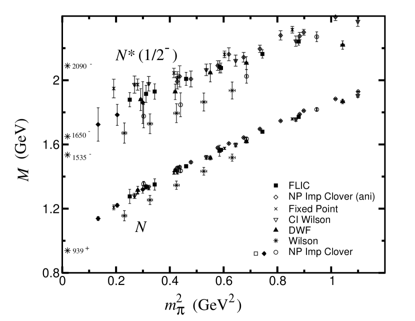
Figure 1: Masses of the nucleon ($N$) and the lowest $J^{P}={1\over 2}^{-}$ excitation (“$N^{*}$”). The FLIC and Wilson results are from Ref CSSM , the DWF DWF , Fixed Point FP , Chirally Improved (CI) Wilson FP , NP improved clover RICHARDS and NP improved anisotropic clover Nakajima:2001js results are shown for comparison. The empirical nucleon and low lying $N^{*}({1\over 2}^{-})$ masses are indicated by the asterisks along the ordinate.

In Fig. 1 we show the nucleon and $N^{*}({1\over 2}^{-})$ masses as a function of the pseudoscalar meson mass squared, $m_{\pi}^{2}$. The filled squares indicate the results for the FLIC action, and the stars for the Wilson action CSSM (the Wilson points are obtained from a sample of 50 configurations). We note here that the spatial size of the lattice is $L=1.95$ fm and that from the values of $m_{\pi}$ given in Table 1 of Ref. CSSM we have $m_{\pi}L\geq 5.52$.

For comparison, we also show results from earlier simulations with domain wall fermions (DWF) DWF (filled triangles), a nonperturbatively (NP) improved clover action on anisotropic lattices at three different lattice spacings Nakajima:2001js (open diamonds), an NP improved clover action at $\beta=6.2$ RICHARDS (open squares, open circles and filled diamonds), and results using Fixed Point (FP) (crosses) and Chirally Improved (CI) (open inverted triangles) FP fermion actions. The scatter of the different NP improved results is due to different source smearing and volume effects: the open squares are obtained by using fuzzed sources and local sinks, the open circles use Jacobi smearing at both the source and sink, while the filled diamonds, which extend to smaller quark masses, are obtained from a larger lattice ($32^{3}\times 64$) using Jacobi smearing. The empirical masses of the nucleon and the three lowest ${1\over 2}^{-}$ excitations are indicated by the asterisks along the ordinate. In an unquenched calculation, the results may shift by the order of $10\%$ compared with a quenched calculation YOUNG .

There is excellent agreement between the different improved actions for the nucleon mass, in particular between the FLIC CSSM , DWF DWF , NP improved clover Nakajima:2001js ; RICHARDS , FP and CI FP results. On the other hand, the Wilson results lie systematically low in comparison to these due to the large ${\cal O}(a)$ errors in this action FATJAMES . A similar pattern is repeated for the $N^{*}({1\over 2}^{-})$ masses. Namely, the FLIC, DWF, NP improved clover, FP and CI masses are in good agreement with each other, while the Wilson results again lie systematically lower. A mass splitting of around 400 MeV is clearly visible between the $N$ and $N^{*}$ for all actions, including the Wilson action, despite its poor chiral properties. Furthermore, the trend of the $N^{*}({1\over 2}^{-})$ data with decreasing $m_{\pi}$ is consistent with the approach to the mass of the lowest-lying physical negative parity $N^{*}$ states.

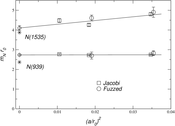
Figure 2: The masses of the lowest-lying positive- and negative-parity baryons in units of $r_{0}^{-1}$ versus $a^{2}$ in units of $r_{0}^{2}$, where $r_{0}$ is Sommer’s scale SOMMER . The lines are linear fits in $a^{2}/r_{0}^{2}$ to the positive- and negative-parity baryon masses; different plotting symbols correspond to different types of smearing. Also shown are the physical values.

In the case of the NP-improved clover fermion action, with ${\cal O}(a^{2})$ discretisation errors, the calculation has been performed at three values of the lattice spacing, enabling a continuum extrapolation to be performed RICHARDS . This is shown in Fig. 2, although it should be noted that a simple linear chiral extrapolation was performed in this calculation. There is a suggestion of a somewhat larger lattice spacing dependence for the higher excited resonance, emphasising the need to perform a careful analysis of systematic uncertainties in future calculations.

Figure 3 shows the mass of the $J^{P}={1\over 2}^{+}$ states (the excited state is denoted by “$N^{\prime}(1/2^{+})$”). As is long known, the positive parity $\chi_{2}$ interpolating field does not have good overlap with the nucleon ground state DEREK and a correlation matrix analysis confirms this result CSSM , as discussed below. It has been speculated that $\chi_{2}$ may have overlap with the lowest ${1\over 2}^{+}$ excited state, the $N^{*}(1440)$ Roper resonance DWF . In addition to the FLIC and Wilson results from the present analysis, we also show in Fig. 3 the DWF results DWF , and those from an earlier analysis with Wilson fermions together with the operator product expansion (OPE) DEREK . The physical values of the lowest three ${1\over 2}^{+}$ excitations of the nucleon are indicated by the asterisks.

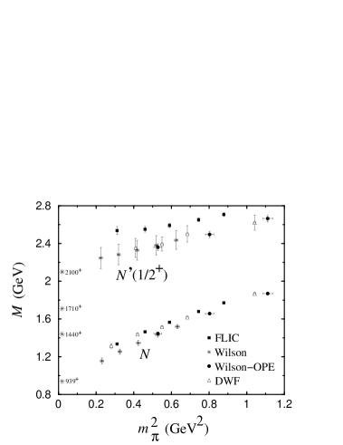
Figure 3: Masses of the nucleon, and the lowest $J^{P}={1\over 2}^{+}$ excitation (“$N^{\prime}$”). The FLIC results CSSM are compared with the DWF DWF and Wilson-OPE DEREK analyses, as well as with the Wilson results from Ref. CSSM . The empirical nucleon and low lying $N^{*}({1\over 2}^{+})$ masses are indicated by asterisks, with physical masses given in MeV.

The most striking feature of the data is the relatively large excitation energy of the $N^{\prime}({1\over 2}^{+})$, some 1 GeV above the nucleon. There is little evidence, therefore, that this state is the $N^{*}(1440)$ Roper resonance. While it is possible that the Roper resonance may have a strong nonlinear dependence on the quark mass at $m_{\pi}^{2}\sim 0.2$ GeV², arising from, for example, pion loop corrections, it is unlikely that this behaviour would be so dramatically different from that of the $N^{*}(1535)$ so as to reverse the level ordering obtained from the lattice. A more likely explanation is that the $\chi_{2}$ interpolating field does not have good overlap with either the nucleon or the $N^{*}(1440)$, but rather (a combination of) excited ${1\over 2}^{+}$ state(s).

Recall that in a constituent quark model in a harmonic oscillator basis, the mass of the lowest mass state with the Roper quantum numbers is higher than the lowest $P$-wave excitation. It seems that neither the lattice data (at large quark masses and with our interpolating fields) nor the constituent quark model have good overlap with the Roper resonance. Better overlap with the Roper is likely to require more exotic interpolating fields.

As mentioned in Section 2, Lee et al. BAYESIAN have performed a calculation using overlap fermions with pion masses down to $\sim 180$ MeV. Using new constrained curve fitting techniques, they extract excited states from a single correlation function calculated with the standard nucleon interpolating field in Eq. (18). The results from this calculation exhibit a dramatic drop in the mass of the first excited ${1\over 2}^{+}$ state of the nucleon at light pion masses, reversing the level ordering of the first ${1\over 2}^{+}$ and ${1\over 2}^{-}$ excited states. It is important, however, that this result be shown to be independent of the constrained curve fitting techniques adopted for this analysis. A correlation matrix analysis involving several operators would shed considerable light on this issue.

Recently there has also been speculation that the Roper resonance suffers from large finite volume errors Sasaki:2003xc . To study this issue, the authors of Ref. Sasaki:2003xc calculate the nucleon and its first positive and negative parity excitations on three different lattice volumes ($La=1.5,\,2.2$ and 3.0 fm). Using Maximum Entropy Methods, they find that on large volume lattices ($\mathrel{\hbox to0.0pt{\raise 2.20013pt\hbox{$>$}\hss}{\lower 2.20013pt\hbox{$\sim$}}}3.0$ fm) the mass of the ${1\over 2}^{+}$ excited nucleon state is reduced. A similar analysis remains to be performed for the first ${1\over 2}^{-}$ nucleon state obtained from the same fermion action. At present Wilson fermion scaling violations allow the ${1\over 2}^{+}$ excited nucleon state to sit lower than the first ${1\over 2}^{-}$ nucleon state obtained from the improved DWF action. It is essential to compare the masses of these states using the same fermion actions to remove systematic errors such as these. Similarly, a correlation matrix analysis involving several operators remains desirable.

The BGR Collaboration has performed a calculation of the excited nucleon spectrum on two lattice volumes ($La\simeq 1.8$ and 2.4 fm) using Fixed Point and Chirally Improved Wilson fermions FP . Using three different operators to create the nucleon states, the lowest two states in both the ${1\over 2}^{+}$ and ${1\over 2}^{-}$ channels are extracted using a $3\times 3$ correlation matrix. The eigenvectors and eigenvalues determined from the correlation matrix analysis should correspond to the solutions of Eq. (4). It is unclear, however, whether the constraints which have been employed in Ref. FP are physical, and in particular whether the eigenvectors correspond to the optimal projections onto physical states defined by the eigenvectors $u$ of Eq. (4). With this caveat, a splitting between the two ${1\over 2}^{-}$ states is identified and the excited ${1\over 2}^{+}$ state is observed to sit above the ${1\over 2}^{-}$ states, in agreement with Ref. CSSM (see next section). The results on two volumes do not exhibit any volume dependence.

In the next section we present results from a $2\times 2$ correlation matrix analysis using FLIC fermions on a single lattice volume.

6.3 Resolving the resonances

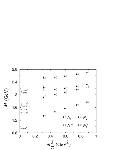
Figure 4: Masses of the $J^{P}={1\over 2}^{+}$ and ${1\over 2}^{-}$ nucleon states, for the FLIC action CSSM . The positive (negative) parity states are labeled $N_{1}$ ($N_{1}^{*}$) and $N_{2}$ ($N_{2}^{*}$). The results from the projection of the correlation matrix are shown by the filled symbols, whereas the results from the standard fits to the $\chi_{1}\overline{\chi}_{1}$ and $\chi_{2}\overline{\chi}_{2}$ correlation functions are shown by the open symbols (offset to the right for clarity). Empirical masses of the low lying ${1\over 2}^{\pm}$ states are indicated by the asterisks.

The mass splitting between the two lightest $N^{*}({1\over 2}^{-})$ states ($N^{*}(1535)$ & $N^{*}(1650)$) can be studied by considering the odd parity content of the $\chi_{1}$ and $\chi_{2}$ interpolating fields in Eqs. (18) and (19). Recall that the “diquarks” in $\chi_{1}$ and $\chi_{2}$ couple differently to spin, so that even though the correlation functions built up from the $\chi_{1}$ and $\chi_{2}$ fields will be made up of a mixture of many excited states, they will have dominant overlap with different states DEREK ; LL . By using the correlation-matrix techniques described in Ref. CSSM (see also Appendix), two separate mass states are extracted from the $\chi_{1}$ and $\chi_{2}$ interpolating fields. The results from the correlation matrix analysis are shown by the filled symbols in Fig. 4, and are compared to the standard “naive” fits performed directly on the diagonal correlation functions, $\chi_{1}\overline{\chi}_{1}$ and $\chi_{2}\overline{\chi}_{2}$, indicated by the open symbols.

The results indicate that indeed the $N^{*}({1\over 2}^{-})$ largely corresponding to the $\chi_{2}$ field (labeled “$N_{2}^{*}$”) lies above the $N^{*}({1\over 2}^{-})$ which can also be isolated via Euclidean time evolution with the $\chi_{1}$ field (“$N_{1}^{*}$”) alone. The masses of the corresponding positive parity states, associated with the $\chi_{1}$ and $\chi_{2}$ fields (labeled “$N_{1}$” and “$N_{2}$”, respectively) are shown for comparison. For reference, we also list the experimentally measured values of the low-lying ${1\over 2}^{\pm}$ states. It is interesting to note that the mass splitting between the positive parity $N_{1}$ and negative parity $N_{1,2}^{*}$ states (roughly 400–500 MeV) is similar to that between the $N_{1,2}^{*}$ and the positive parity $N_{2}$ state, reminiscent of a constituent quark–harmonic oscillator picture.

Turning to the strange sector, in Fig. 6 we show the masses of the positive and negative parity $\Sigma$ baryons calculated from the FLIC action CSSM compared with the physical masses of the known positive and negative parity states. The pattern of mass splittings is similar to that found in Fig. 4 for the nucleon. Namely, the ${1\over 2}^{+}$ state associated with the $\chi_{1}$ field appears consistent with the empirical $\Sigma(1193)$ ground state, while the ${1\over 2}^{+}$ state associated with the $\chi_{2}$ field lies significantly above the observed first (Roper-like) ${1\over 2}^{+}$ excitation, $\Sigma^{*}(1660)$. There is also evidence for a mass splitting between the two negative parity states, similar to that in the nonstrange sector.

The spectrum of the strangeness –2 positive and negative parity $\Xi$ hyperons is displayed in Fig. 6. Once again, the pattern of calculated masses repeats that found for the $\Sigma$ and $N$ masses in Figs. 4 and 6, and for the respective coupling coefficients CSSM . The empirical masses of the physical $\Xi^{*}$ baryons are denoted by asterisks. However, for all but the ground state $\Xi(1318)$, the $J^{P}$ values are not known.

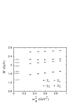
Figure 5: As in Fig. 4 but for the $\Sigma$ baryons.

Figure 6: As in Fig. 4 but for the $\Xi$ baryons. The $J^{P}$ values of the excited states marked with “?” are undetermined.

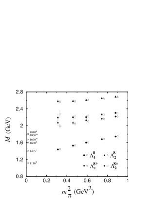
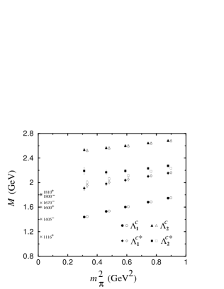
Figure 7: As in Fig. 4 but for the $\Lambda$ states obtained using the $\Lambda^{8}$ interpolating field.

Figure 8: As in Fig. 4 but for the $\Lambda$ states obtained using the $\Lambda^{c}$ interpolating field.

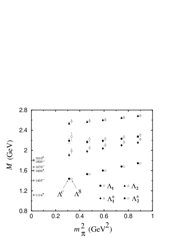
Figure 9: Masses of the positive and negative parity $\Lambda$ states, for the octet $\Lambda^{8}$ (open symbols) and “common” $\Lambda^{c}$ (filled symbols) interpolating fields with the FLIC action CSSM . The positive (negative) parity states labeled $\Lambda_{1}$ ($\Lambda_{1}^{*}$) and $\Lambda_{2}$ ($\Lambda_{2}^{*}$) are the two states obtained from the correlation matrix analysis of the $\chi_{1}^{\Lambda}$ and $\chi_{2}^{\Lambda}$ interpolating fields. Empirical masses of the low lying ${1\over 2}^{\pm}$ states are indicated by the asterisks.

Finally, we consider the $\Lambda$ hyperons. In Figs. 8 and 8 we compare results obtained from the $\Lambda^{8}$ and $\Lambda^{c}$ interpolating fields, respectively, using the two different techniques for extracting masses. A direct comparison between the positive and negative parity masses for the $\Lambda^{8}$ (open symbols) and $\Lambda^{c}$ (filled symbols) states extracted from the correlation matrix analysis, is shown in Fig. 9. A similar pattern of mass splittings to that for the $N^{*}$ spectrum of Fig. 8 is observed. In particular, the negative parity $\Lambda_{1}^{*}$ state (diamonds) lies $\sim 400$ MeV above the positive parity $\Lambda_{1}$ ground state (circles), for both the $\Lambda^{8}$ and $\Lambda^{c}$ fields. There is also clear evidence of a mass splitting between the $\Lambda_{1}^{*}$ (diamonds) and $\Lambda_{2}^{*}$ (squares).

Using the naive fitting scheme (open symbols in Figs. 8 and 8) misses the mass splitting between $\Lambda_{1}^{*}$ and $\Lambda_{2}^{*}$ for the “common” interpolating field. Only after performing the correlation matrix analysis is it possible to resolve two separate mass states, as seen by the filled symbols in Fig. 8. As for the other baryons, there is little evidence that the $\Lambda_{2}$ (triangles) has any significant overlap with the first positive parity excited state, $\Lambda^{*}(1600)$ (cf. the Roper resonance, $N^{*}(1440)$, in Fig. 4).

While it seems plausible that nonanalyticities in a chiral extrapolation MASSEXTR of $N_{1}$ and $N_{1}^{*}$ results could eventually lead to agreement with experiment, the situation for the $\Lambda^{*}(1405)$ is not as compelling. Whereas a 150 MeV pion-induced self energy is required for the $N_{1},\ N_{1}^{*}$ and $\Lambda_{1}$, 400 MeV is required to approach the empirical mass of the $\Lambda^{*}(1405)$. This may not be surprising for the octet fields, as the $\Lambda^{*}(1405)$, being an SU(3) flavour singlet, may not couple strongly to an SU(3) octet interpolating field. Indeed, there is some evidence of this in Fig. 9. This large discrepancy of 400 MeV suggests that relevant physics giving rise to a light $\Lambda^{*}(1405)$ may be absent from simulations in the quenched approximation. The behaviour of the $\Lambda_{1,2}^{*}$ states may be modified at small values of the quark mass through nonlinear effects associated with Goldstone boson loops including the strong coupling of the $\Lambda^{*}(1405)$ to $\Sigma\pi$ and $\bar{K}N$ channels. While some of this coupling will survive in the quenched approximation, generally the couplings are modified and suppressed YOUNG ; SHARPE . It is also interesting to note that the $\Lambda_{1}^{*}$ and $\Lambda_{2}^{*}$ masses display a similar behaviour to that seen for the $\Xi_{1}^{*}$ and $\Xi_{2}^{*}$ states, which are dominated by the heavier strange quark. Alternatively, the study of more exotic interpolating fields may indicate the the $\Lambda^{*}(1405)$ does not couple strongly to $\chi_{1}$ or $\chi_{2}$. Investigations at lighter quark masses involving quenched chiral perturbation theory will assist in resolving these issues.

6.4 Spin-$\frac{3}{2}$ Baryons

Figure 10: Masses of the spin projected $N{3\over 2}^{-}$ (filled triangles), $N{3\over 2}^{+}$ (filled inverted triangles), $N{1\over 2}^{+}$ (filled circles), and $N{1\over 2}^{-}$ (filled squares) isospin-${1\over 2}$ states CSSM32 . For comparison, previous results from the direct calculation of the $N{1\over 2}^{+}$ (open circles) and $N{1\over 2}^{-}$ (open squares) from Fig. 1 are also shown. The empirical values of the masses of the $N{1\over 2}^{+}\,(939)$, $N{1\over 2}^{-}\,(1535)$, $N{3\over 2}^{-}\,(1520)$ and $N{3\over 2}^{+}\,(1720)$ are indicated (in MeV) on the left-hand-side at the physical pion mass.

The interpolating field defined in Eq. (58) has overlap with spin-$\frac{1}{2}$ and spin-$\frac{3}{2}$ states of both parities. After performing appropriate spin projections on the correlation functions, the masses of the $N{3\over 2}^{\pm}$ and $N{1\over 2}^{\pm}$ states are extracted and displayed in Fig. 10 as a function of $m_{\pi}^{2}$. Earlier results for the $N\frac{1}{2}^{\pm}$ states using the standard spin-$1\over 2$ interpolating field FATJAMES ; CSSM from Eq. (18) are also shown with open symbols in Fig. 10 for reference. It is encouraging to note the agreement between the spin-projected ${1\over 2}^{\pm}$ states obtained from the spin-${3\over 2}$ interpolating field in Eq. (58) and the earlier ${1\over 2}^{\pm}$ results from the same gauge field configurations. We also observe that the $N\frac{3}{2}^{-}$ state has approximately the same mass as the spin-projected $N\frac{1}{2}^{-}$ state which is consistent with the experimentally observed masses. The results for the $N\frac{3}{2}^{-}$ state in Fig. 10 indicate a clear mass splitting between the $N{3\over 2}^{+}$ and $N{3\over 2}^{-}$ states obtained from the spin-${3\over 2}$ interpolating field, with a mass difference around 300 MeV. This is slightly larger than the experimentally observed mass difference of 200 MeV.

Turning now to the isospin-${3\over 2}$ sector, results for the $\Delta{3\over 2}^{+}$ and $\Delta{3\over 2}^{-}$ masses are shown in Fig. 11 as a function of $m_{\pi}^{2}$. The trend of the $\Delta{3\over 2}^{+}$ data points with decreasing $m_{\pm}$ is clearly towards the $\Delta(1232)$, although some nonlinearity with $m_{\pi}^{2}$ is expected near the chiral limit MASSEXTR ; YOUNG . The mass of the $\Delta{3\over 2}^{-}$ lies some 500 MeV above that of its parity partner, although with somewhat larger errors.

Figure 11: Masses of the spin-projected $\Delta{3\over 2}^{\pm}$ and $\Delta{1\over 2}^{\pm}$ isospin-${3\over 2}$ resonances CSSM32 . The empirical values of the masses of the $\Delta^{3/2^{+}}(1232)$, $\Delta{3\over 2}^{-}(1700)$, $\Delta{1\over 2}^{-}(1620)$ and $\Delta{1\over 2}^{+}(1910)$ are shown (in MeV) on the left-hand-side at the physical pion mass.

After performing a spin projection to extract the $\Delta{1\over 2}^{\pm}$ states a discernible, but noisy, signal is detected. This indicates that the interpolating field in Eq. (63) has only a small overlap with spin-$\frac{1}{2}$ states. However, with 400 configurations we are able to extract a mass for the spin-$\frac{1}{2}$ states at early times, shown in Fig. 11. Here we see the larger error bars associated with the $\Delta{1\over 2}^{\pm}$ states. The lowest excitation of the ground state, namely the $\Delta{1\over 2}^{-}$, has a mass $\sim 350$–400 MeV above the $\Delta{3\over 2}^{+}$, with the $\Delta{3\over 2}^{-}$ possibly appearing heavier. The $\Delta{1\over 2}^{+}$ state is found to lie $\sim 100$–200 MeV above these, although the signal becomes weak at smaller quark masses. This level ordering is consistent with that observed in the empirical mass spectrum, which is also shown in the figure.

The $N{1\over 2}^{-}$ and $\Delta{1\over 2}^{-}$ states will decay to $N\pi$ in $S$-wave even in the quenched approximation QQCD . For all quark masses considered here, with the possible exception of the lightest quark, this decay channel is closed for the nucleon. While there may be some spectral strength in the decay mode, we are unable to separate it from the resonant spectral strength.

The $N{3\over 2}^{+}$ and $\Delta{1\over 2}^{+}$ states will decay to $N\pi$ in $P$-wave, while $N{3\over 2}^{-}$ and $\Delta{3\over 2}^{-}$ states will decay to $N\pi$ in $D$-wave. Since the decay products of each of these states must then have equal and opposite momentum and energy given by

$$E^{2}=M^{2}+\left(\frac{2\pi}{aL}\right)^{2},$$

these states are stable in the present calculations.

7 Conclusions

The increasing effort given to the study of the excited baryon and meson spectrum by the lattice community reflects the appreciation that the determination of the spectrum provides vital clues to the dynamics of QCD, and the mechanisms of confinement. The $N^{*}$ spectrum in particular has several features, such as the anomalously light $N^{*}(1440)$ Roper resonance and the $J^{P}={1\over 2}^{-}$ $\Lambda(1405)$, that defy a straightforward interpretation within the quark model, and whose understanding can help to resolve the competing pictures of hadron structure. The impetus to study the $N^{*}$ resonances has also strengthened following the observation of the $S=+1$, $\Theta^{+}$ pentaquark state, whose properties remain essentially unknown, but whose various interpretations offer vastly different pictures of baryon structure.

In these lectures, we have described the techniques required to compute the $N^{*}$ spectrum in lattice QCD, and given an overview of the current status of lattice calculations. The lightest states of both parities for spin $1/2$ and spin $3/2$ have been successfully resolved in the quenched approximation to QCD in both the nucleon (isospin-${1\over 2}$) and $\Delta$ (isospin-${3\over 2}$) sectors, and in general the level ordering, albeit at relatively large pseudoscalar masses, $m_{\pi}\geq 500~{}{\rm MeV}$, is in accord with that observed experimentally. At these large pseudoscalar masses the spectrum largely follows quark-model expectations.

It is important to appreciate that most current spectroscopy calculations have employed essentially “$S$-wave” quark propagators. The measurement of a wider basis of interpolating operators will be an important element of future studies, and the technology to construct such operators with lattice symmetry properties has now been developed. An important by-product of such studies will be insight into the quark and gluon structure of such hadrons.

The realisation that hadronic physics at physical values of the pion mass is very different from that at $m_{\pi}\geq 300~{}{\rm MeV}$, and the consequent need to correctly account for the chiral properties of the theory, have been some of the most important developments in lattice QCD of recent years. FLIC fermions and the development of fermions having an exact analogue of chiral symmetry provide the means to attain such pion masses. There are suggestions that such radically different behaviour at light quark masses has been seen in the excited nucleon sector. With the development of exact dynamical fat-link fermion algorithms Kamleh:2004xk ; Kamleh:2004ti ; Kamleh:2003wb , FLIC fermions provide tremendous promise for accessing the light-quark mass regime of full QCD.

The continuation to physical values of the light quark masses poses extra challenges to the calculation of the resonance spectrum. The excited states are no longer stable under the strong interaction at sufficiently light quark masses. Even in the quenched approximation, this instability is manifest through non-unitary behaviour in the correlators and through additional non-analytic terms in the chiral expansion of nucleon masses Morel:2003fj . The means to study the full spectrum, including the scattering lengths of multi-particle states, is in principle known, relying on examining the finite-volume shift in the two-particle spectrum. However, the method is computationally very demanding, requiring the measurement of many operators.

With the realisation of large-scale computing facilities expected over the next several years, we can expect many of these endevours to come to fruition. An exciting era for baryon spectroscopy on the lattice lays ahead.

8 Appendix - Correlation Matrix Analysis

In this section we outline the correlation matrix formalism for calculations of masses, coupling strengths and optimal interpolating fields. After demonstrating that the correlation functions are real, we proceed to show how a matrix of such correlation functions may be used to isolate states corresponding to different masses, and also to give information about the coupling of the operators to each of these states (see also Ref. CSSM ).

8.1 The $U+U^{\ast}$ method

A lattice QCD correlation function for the operator $\chi_{i}\overline{\chi}_{j}$, where $\chi_{i}$ is the $i$-th interpolating field for a particular baryon (e.g. $\chi_{2}^{p+}$ in Section 5.2), can be written as

$${\cal G}_{ij} \equiv \left\langle\Omega|T(\chi_{i}\overline{\chi}_{j})|\Omega\right\rangle$$ (86)

$$= \frac{\int{\cal D}U{\cal D}\bar{\psi}{\cal D}\psi e^{-S[U,\bar{\psi},\psi]}\chi_{i}\overline{\chi}_{j}}{\int{\cal D}U{\cal D}\bar{\psi}{\cal D}\psi e^{-S[U,\bar{\psi},\psi]}}\,,$$ (87)

where spinor indices and spatial coordinates are suppressed for ease of notation. The fermion and gauge actions can be separated such that $S[U,\bar{\psi},\psi]=S_{G}[U]+\bar{\psi}M[U]\psi$. Integration over the Grassmann variables $\bar{\psi}$ and $\psi$ then gives

$${\cal G}_{ij}\ =\ \frac{\int{\cal D}Ue^{-S_{G}[U]}\det(M[U])H_{ij}[U]}{\int{\cal D}Ue^{-S_{G}[U]}\det(M[U])}\ ,$$ (88)

where the term $H_{ij}$ stands for the sum of all full contractions of $\chi_{i}\overline{\chi}_{j}$. The pure gauge action $S_{G}$ and the fermion matrix $M$ satisfy

$$S_{G}[U]=S_{G}[U^{\ast}]\ ,$$ (89)

and

$$\widetilde{C}M[U^{\ast}]\widetilde{C}^{-1}=M^{\ast}[U]\ ,$$ (90)

respectively, where $\widetilde{C}\equiv C\gamma_{5}$.

Using the result of Eq. (90), one has

$$\det\left(M[U^{\ast}]\right) = \det\left(M^{\ast}[U]\right)\ ,$$ (91)

and since ${\rm det}(M[U])$ is real, this leads to

$$\det\left(M[U^{\ast}]\right)={\det\left(M[U]\right)}\ .$$ (92)

Thus, $U$ and $U^{\ast}$ are configurations of equal weight in the measure
$\int{\cal D}U{\rm det}(M[U]){\rm exp}\left(-S_{G}[U]\right)$, in which case ${\cal G}_{ij}$ can be written as

$${\cal G}_{ij}=\frac{1}{2}\left(\frac{\int{\cal D}Ue^{-S_{G}[U]}\det(M[U])\left\{H_{ij}[U]+H_{ij}[U^{\ast}]\right\}}{\int{\cal D}Ue^{-S_{G}[U]}\det(M[U])}\right)\,.$$ (93)

Let us define

$$G^{\pm}_{ij}\equiv{\rm tr}[\Gamma_{\pm}{\cal G}_{ij}]\,,$$ (94)

where “$\rm tr$” denotes the spinor trace and $\Gamma_{\pm}$ is the parity-projection operator defined in Eq. (17). If ${\rm tr}\left[{\Gamma H_{ij}[U^{\ast}]}\right]={\rm tr}\left[{\Gamma H_{ij}^{\ast}[U]}\right]$, then $G^{\pm}_{ij}$ is real. This can be shown by first noting that $H_{ij}$ will be products of Dirac $\gamma$-matrices, fermion propagators, and link-field operators. In a $\gamma$-matrix representation which is Hermitian, such as the Sakurai representation, $\widetilde{C}\gamma_{\mu}\widetilde{C}^{-1}=\gamma_{\mu}^{*}$. Fermion propagators have the form $M^{-1}$, and recalling that since $\widetilde{C}M[U^{\ast}]\widetilde{C}^{-1}$=$M^{\ast}[U]$, then we have $\widetilde{C}M^{-1}[U^{\ast}]\widetilde{C}^{-1}$=$(M^{-1}[U])^{\ast}$. For products of link-field operators $O[U]$ contained in $H_{ij}$, the condition $O[U^{\ast}]=O^{\ast}[U]$ is equivalent to the requirement that the coefficients of all link-products are real. As long as this requirement is enforced, we can then simply proceed by inserting $\widetilde{C}\widetilde{C}^{-1}$ inside the trace to show that the (spinor-traced) correlation functions $G^{\pm}_{ij}$ are real. If one chooses the Dirac representation, then $\widetilde{C}\gamma_{k}\widetilde{C}^{-1}=-\gamma_{k}^{*}$ and $\widetilde{C}\gamma_{0}\widetilde{C}^{-1}=\gamma_{0}^{*}$. Therefore, in the Dirac representation of the $\gamma$-matrices, if $H_{ij}$ contains an even number of spatial $\gamma$-matrices with real coefficients, $G_{ij}^{\pm}$ is purely real; otherwise $G_{ij}^{\pm}$ is purely imaginary.

In summary, the interpolating fields considered here are constructed using only real coefficients and have no spatial $\gamma$-matrices. Therefore, the correlation functions $G^{\pm}_{ij}$ are real. This symmetry is explicitly implemented by including both $U$ and $U^{*}$ in the ensemble averaging used to construct the lattice correlation functions, providing an improved unbiased estimator which is strictly real. This is easily implemented at the correlation function level by observing

$$M^{-1}(\{U_{\mu}^{*}\})=[C\gamma_{5}\,M^{-1}(\{U_{\mu}\})\,(C\gamma_{5})^{-1}]^{*}$$

for quark propagators.

8.2 Recovering Masses, Couplings and Optimal Interpolators

Let us again consider the momentum-space two-point function for $t>0$,

$${\cal G}_{ij}(t,\vec{p})=\sum_{\vec{x}}e^{-i\vec{p}\cdot\vec{x}}\langle\Omega|\chi_{i}(t,\vec{x})\overline{\chi}_{j}(0,\vec{0})|\Omega\rangle\ .$$ (95)

At the hadronic level,

$${\cal G}_{ij}(t,\vec{p}) = \sum_{\vec{x}}e^{-i\vec{p}\cdot\vec{x}}\sum_{\vec{p}^{\prime},s}\sum_{B}\langle\Omega|\chi_{i}(t,\vec{x})|B,p^{\prime},s\rangle$$

$$\times \langle B,p^{\prime},s|\overline{\chi}_{j}(0,\vec{0})|\Omega\rangle\ ,$$

where the $|B,p^{\prime},s\rangle$ are a complete set of states with momentum $p^{\prime}$ and spin $s$

$$\sum_{\vec{p}^{\prime}}\sum_{B}\sum_{s}|B,p^{\prime},s\rangle\langle B,p^{\prime},s|=I\ .$$ (96)

We can make use of translational invariance to write

$${\cal G}_{ij}(t,\vec{p}) = \sum_{\vec{x}}e^{-i\vec{p}\cdot\vec{x}}\sum_{\vec{p}^{\prime}}\sum_{s}\sum_{B}\left\langle\Omega\left|e^{\hat{H}t}e^{-i\hat{\vec{P}}\cdot\vec{x}}\chi_{i}(0)e^{i\hat{\vec{P}}\cdot\vec{x}}e^{-\hat{H}t}\right|B,p^{\prime},s\right\rangle$$ (98)

$$\hskip 113.81102pt\times\left\langle B,p^{\prime},s\left|\overline{\chi}_{j}(0)\right|\Omega\right\rangle$$

$$= \sum_{s}\sum_{B}e^{-{E_{B}t}}\left\langle\Omega|\chi_{i}(0)|B,p,s\rangle\langle B,p,s|\overline{\chi}_{j}(0)|\Omega\right\rangle\ .$$ (99)

It is convenient in the following discussion to label the states which have the $\chi$ interpolating field quantum numbers and which survive the parity projection as $|B_{\alpha}\rangle$ for $\alpha=1,2,\cdots,N$. In general the number of states, $N$, in this tower of excited states may be infinite, but we will only ever need to consider a finite set of the lowest such states here. After selecting zero momentum, $\vec{p}=0$, the parity-projected trace of this object is then

$$G^{\pm}_{ij}(t)={\rm tr}[\Gamma_{\pm}{\cal G}_{ij}(t,\vec{0})]=\sum_{\alpha=1}^{N}e^{-{m_{\alpha}}t}\lambda^{\alpha}_{i}\overline{\lambda}^{\alpha}_{j}\ ,$$ (100)

where $\lambda^{\alpha}_{i}$ and $\overline{\lambda}^{\alpha}_{j}$ are coefficients denoting the couplings of the interpolating fields $\chi_{i}$ and $\overline{\chi}_{j}$, respectively, to the state $\left|B_{\alpha}\right\rangle$. If we use identical source and sink interpolating fields then it follows from the definition of the coupling strength that $\overline{\lambda}^{\alpha}_{j}=(\lambda^{\alpha}_{j})^{*}$ and from Eq. (100) we see that $G^{\pm}_{ij}(t)=[G^{\pm}_{ji}(t)]^{*}$, i.e., $G^{\pm}$ is a Hermitian matrix. If, in addition, we use only real coefficients in the link products, then $G^{\pm}$ is a real symmetric matrix. For the correlation matrices that we construct, we have real link coefficients but smeared sources and point sinks. Consequently, $G$ is a real but non-symmetric matrix. Since $G^{\pm}$ is a real matrix for the infinite number of possible choices of interpolating fields with real coefficients, then we can take $\lambda^{\alpha}_{i}$ and $\overline{\lambda}^{\alpha}_{j}$ to be real coefficients without loss of generality.

Suppose now that we have $M$ creation and annihilation operators, where $M<N$. We can then form an $M\times M$ approximation to the full $N\times N$ matrix $G$. At this point there are two options for extracting masses. The first is the standard method for calculation of effective masses at large $t$ described in Section 5.1. The second option is to extract the masses through a correlation-matrix procedure MCNEILE .

Let us begin by considering the ideal case where we have $N$ interpolating fields with the same quantum numbers, but which give rise to $N$ linearly independent states when acting on the vacuum. In this case we can construct $N$ ideal interpolating source and sink fields which perfectly isolate the $N$ individual baryon states $|B_{\alpha}\rangle$,

$$\overline{\phi}^{\alpha} = \sum_{i=1}^{N}u^{\alpha}_{i}\ \overline{\chi}_{i}\ ,$$ (101)

$$\phi^{\alpha} = \sum_{i=1}^{N}v^{\ast\alpha}_{i}\ \chi_{i}\ ,$$ (102)

such that

$$\left\langle B_{\beta}\right|\overline{\phi}^{\alpha}\left|\Omega\right\rangle = \delta_{\alpha\beta}\ \overline{z}^{\alpha}\ \overline{u}(\alpha,p,s)\ ,$$ (103)

$$\left\langle\Omega\right|\phi^{\alpha}\left|B_{\beta}\right\rangle = \delta_{\alpha\beta}\ z^{\alpha}\ u(\alpha,p,s)\ ,$$ (104)

where $z^{\alpha}$ and $\overline{z}^{\alpha}$ are the coupling strengths of $\phi^{\alpha}$ and $\overline{\phi}^{\alpha}$ to the state $|B_{\alpha}\rangle$. The coefficients $u_{i}^{\alpha}$ and $v_{i}^{\ast\alpha}$ in Eqs. (102) may differ when the source and sink have different smearing prescriptions, again indicated by the differentiation between $z^{\alpha}$ and $\overline{z}^{\alpha}$. For notational convenience for the remainder of this discussion repeated indices $i,j,k$ are to be understood as being summed over. At $\vec{p}=0$, it follows that,

$$G^{\pm}_{ij}(t)\ u^{\alpha}_{j} = \left(\sum_{\vec{x}}{\rm tr}\left[\Gamma_{\pm}\left\langle\Omega\right|\chi_{i}\overline{\chi}_{j}\left|\Omega\right\rangle\right]\right)u^{\alpha}_{j}$$ (105)

$$= \lambda^{\alpha}_{i}\overline{z}^{\alpha}e^{-m_{\alpha}t}.$$ (106)

The only $t$-dependence in this expression comes from the exponential term, which leads to the recurrence relationship

$$G^{\pm}_{ij}(t)\,u^{\alpha}_{j}=e^{m_{\alpha}}G^{\pm}_{ik}(t+1)\,u^{\alpha}_{k}\ ,$$ (107)

which can be rewritten as

$$[G^{\pm}(t+1)]_{ki}^{-1}G^{\pm}_{ij}(t)\,u^{\alpha}_{j}=e^{m_{\alpha}}\,u^{\alpha}_{k}\ .$$ (108)

This is recognised as an eigenvalue equation for the matrix $[G^{\pm}(t+1)]^{-1}G^{\pm}(t)$ with eigenvalues $e^{m_{\alpha}}$ and eigenvectors $u^{\alpha}$. Hence the natural logarithms of the eigenvalues of $[G^{\pm}(t+1)]^{-1}G^{\pm}(t)$ are the masses of the $N$ baryons in the tower of excited states corresponding to the selected parity and the quantum numbers of the $\chi$ fields. The eigenvectors are the coefficients of the $\chi$ fields providing the ideal linear combination for that state. Note that since here we use only real coefficients in our link products, then $[G^{\pm}(t+1)]^{-1}G^{\pm}(t)$ is a real matrix and so $u^{\alpha}$ and $v^{\alpha}$ will be real eigenvectors. It also then follows that $z^{\alpha}$ and $\overline{z}^{\alpha}$ will be real. These coefficients are examined in detail in the following section.

One can also construct the equivalent left-eigenvalue equation to recover the $v$ vectors, providing the optimal linear combination of annihilation interpolators,

$$v^{\ast\alpha}_{k}G^{\pm}_{kj}(t)=e^{m_{\alpha}}v^{\ast\alpha}_{i}G^{\pm}_{ij}(t+1)\ .$$ (109)

Recalling Eq. (105), one finds:

$$G^{\pm}_{ij}(t)\ u^{\alpha}_{j} = \overline{z}^{\alpha}\lambda^{\alpha}_{i}e^{-m_{\alpha}t}\ ,$$ (110)

$$v^{\ast\alpha}_{i}\ G^{\pm}_{ij}(t) = {z}^{\alpha}\overline{\lambda}^{\alpha}_{j}e^{-m_{\alpha}t}\ ,$$ (111)

$$v^{\ast\alpha}_{k}\ G^{\pm}_{kj}(t)G^{\pm}_{il}(t)\ u^{\alpha}_{l} = z^{\alpha}\overline{z}^{\alpha}\lambda^{\alpha}_{i}\overline{\lambda}^{\alpha}_{j}e^{-2m_{\alpha}t}\ .$$ (112)

The definitions of Eqs. (104) imply

$$v^{\ast\alpha}_{i}\ G^{\pm}_{ij}(t)\ u^{\alpha}_{j}=z^{\alpha}\overline{z}^{\alpha}e^{-m_{\alpha}t},$$ (113)

indicating the eigenvectors may be used to construct a correlation function in which a single state mass $m_{\alpha}$is isolated and which can be analysed using the methods of Section II. We refer to this as the projected correlation function in the following. Combining Eqs. (112) and (113) leads us to the result

$$\frac{v^{\ast\alpha}_{k}\ G_{kj}(t)G_{il}(t)\ u^{\alpha}_{l}}{v^{\ast\alpha}_{k}G_{kl}(t)u^{\alpha}_{l}}=\lambda^{\alpha}_{i}\overline{\lambda}^{\alpha}_{j}e^{-m_{\alpha}t}\ .$$ (114)

By extracting all $N^{2}$ such ratios, we can exactly recover all of the real couplings $\lambda^{\alpha}_{i}$ and $\overline{\lambda}^{\alpha}_{j}$ of $\chi_{i}$ and $\overline{\chi}_{j}$ respectively to the state $|B_{\alpha}\rangle$. Note that throughout this section no assumptions have been made about the symmetry properties of $G_{ij}^{\pm}$. This is essential due to our use of smeared sources and point sinks.

In practice we will only have a relatively small number, $M<N$, of interpolating fields in any given analysis. These $M$ interpolators should be chosen to have good overlap with the lowest $M$ excited states in the tower and we should attempt to study the ratios in Eq. (114) at early to intermediate Euclidean times, where the contribution of the $(N-M)$ higher mass states will be suppressed but where there is still sufficient signal to allow the lowest $M$ states to be seen. This procedure will lead to an estimate for the masses of each of the lowest $M$ states in the tower of excited states. Of these $M$ predicted masses, the highest will in general have the largest systematic error while the lower masses will be most reliably determined. Repeating the analysis with varying $M$ and different combinations of interpolating fields will give an objective measure of the reliability of the extraction of these masses.

In our case of a modest $2\times 2$ correlation matrix ($M=2$) we take a cautious approach to the selection of the eigenvalue analysis time. As already explained, we perform the eigenvalue analysis at an early to moderate Euclidean time where statistical noise is suppressed and yet contributions from at least the lowest two mass states is still present. One must exercise caution in performing the analysis at too early a time, as more than the desired $M=2$ states may be contributing to the $2\times 2$ matrix of correlation functions.

We begin by projecting a particular parity, and then investigate the effective mass plots of the elements of the correlation matrix. Using the covariance-matrix based $\chi^{2}/N_{\rm DF}$, we identify the time slice at which all correlation functions of the correlation matrix are dominated by a single state. In practice, this time slice is determined by the correlator providing the lowest-lying effective mass plot. The eigenvalue analysis is performed at one time slice earlier, thus ensuring the presence of multiple states in the elements of the correlation function matrix, minimising statistical uncertainties, and hopefully providing a clear signal for the analysis. In this approach minimal new information has been added, providing the best opportunity that the $2\times 2$ correlation matrix is indeed dominated by 2 states. The left and right eigenvectors are determined and used to project correlation functions containing a single state from the correlation matrix as indicated in Eq. (113). These correlation functions are then subjected to the same covariance-matrix based $\chi^{2}/N_{\rm DF}$ analysis to identify new acceptable fit windows for determining the masses of the resonances.

References

- (1) V. Burkert et al., Few Body Syst. Suppl. 11 (1999) 1.
- (2) http://www.lepp.cornell.edu/public/CLEO/spoke/CLEOc/ .
- (3) http://www.gsi.de/zukunftsprojekt/experimente/hesr-panda/ .
- (4) http://www.jlab.org/Hall-D/ .
- (5) S. Capstick and W. Roberts, Prog. Part. Nucl. Phys. 45 (2000) S241.
- (6) N. Isgur and G. Karl, Phys. Lett. B 72 (1977) 109; Phys. Rev. D 19 (1979) 2653.
- (7) Z.-P. Li, V. Burkert and Z.-J. Li, Phys. Rev. D 46 (1992) 70; C. E. Carlson and N. C. Mukhopadhyay, Phys. Rev. Lett. 67 (1991) 3745.
- (8) P. A. M. Guichon, Phys. Lett. B 164 (1985) 361.
- (9) O. Krehl, C. Hanhart, S. Krewald and J. Speth, Phys. Rev. C 62 (2000) 025207.
- (10) R. H. Dalitz and J. G. McGinley, in Low and Intermediate Energy Kaon-Nucleon Physics, ed. E. Ferarri and G. Violini (Reidel, Boston, 1980), p.381; R. H. Dalitz, T.C. Wong and G. Rajasekaran, Phys. Rev. 153 (1967) 1617; E. A. Veit, B. K. Jennings, R. C. Barrett and A. W. Thomas, Phys. Lett. B 137 (1984) 415; E. A. Veit, B. K. Jennings, A. W. Thomas and R. C. Barrett, Phys. Rev. D 31 (1985) 1033; P. B. Siegel and W. Weise, Phys. Rev. C 38 (1988) 2221; N. Kaiser, P. B. Siegel and W. Weise, Nucl. Phys. A594 (1995) 325; E. Oset, A. Ramos and C. Bennhold, Phys. Lett. B 527 (2002) 99 [Erratum-ibid. B 530 (2002) 260].
- (11) D. B. Leinweber, A. W. Thomas, K. Tsushima and S. V. Wright, Phys. Rev. D 61 (2000) 074502.
- (12) R. D. Young, D. B. Leinweber, A. W. Thomas and S. V. Wright, Phys. Rev. D 66 (2002) 094507.
- (13) D. Morel, B. Crouch, D. B. Leinweber and A. W. Thomas, “Physical baryon resonance spectroscopy from lattice QCD,” arXiv:nucl-th/0309044.
- (14) A. De Rújula, H. Georgi and S.L. Glashow, Phys. Rev. D 12 (1975) 147.
- (15) L. Y. Glozman and D. O. Riska, Phys. Rep. 268 (1996) 263; L. Y. Glozman, Phys. Lett. B 494 (2000) 58.
- (16) D.B. Leinweber, Annals Phys. 198 (1990) 203.
- (17) S. Capstick and N. Isgur, Phys. Rev. D 34 (1986) 2809.
- (18) C. L. Schat, J. L. Goity and N. N. Scoccola, Phys. Rev. Lett. 88 (2002) 102002; C. E. Carlson, C. D. Carone, J. L. Goity and R. F. Lebed, Phys. Rev. D 59 (1999) 114008; J. L. Goity, Phys. Lett. B 414 (1997) 140; D. Pirjol and C. Schat, Phys. Rev. D 67 (2003) 096009.
- (19) See Penta-Quark 2003 Workshop, Jefferson Lab, Virginia (November 2003), http://www.jlab.org/intralab/calendar/archive03/pentaquark/ .
- (20) D.B. Leinweber, A.W. Thomas, K. Tsushima and S.V. Wright, Phys. Rev. D 64 (2001) 094502.
- (21) C.R. Allton et al. [UKQCD Collaboration], Phys. Rev. D 47 (1993) 5128.
- (22) D. B. Leinweber, Phys. Rev. D 51 (1995) 6383.
- (23) M. W. Hecht and T. A. DeGrand, Phys. Lett. B 275 (1992) 435; T. A. DeGrand and M. W. Hecht, Phys. Rev. D 46 (1992) 3937.
- (24) F. X. Lee and D. B. Leinweber, Nucl. Phys. Proc. Suppl. 73 (1999) 258.
- (25) F. X. Lee, Nucl. Phys. Proc. Suppl. 94 (2001) 251.
- (26) N. Nakajima, H. Matsufuru, Y. Nemoto and H. Suganuma, “SU(3) lattice QCD study for octet and decuplet baryon spectra,” arXiv:hep-lat/0204014; Y. Nemoto, N. Nakajima, H. Matsufuru and H. Suganuma, Nucl. Phys. A721 (2003) 879.
- (27) S. Sasaki, T. Blum and S. Ohta, Phys. Rev. D 65 (2002) 074503. S. Sasaki, “Lattice study of nucleon properties with domain wall fermions,” arXiv:hep-lat/0110052.
- (28) D. Kaplan, Phys. Lett. B 288 (1992) 342.
- (29) S. Sasaki, Prog. Theor. Phys. Suppl. 151 (2003) 143; K. Sasaki, S. Sasaki, T. Hatsuda and M. Asakawa, “Excited nucleon spectrum from lattice QCD with maximum entropy method,” arXiv:hep-lat/0309177.
- (30) B. Sheikholeslami and R. Wohlert, Nucl. Phys. B259 (1985) 572.
- (31) D. G. Richards, Nucl. Phys. Proc. Suppl. 94 (2001) 269; M. Göckeler et al. [QCDSF Collaboration], Phys. Lett. B 532 (2002) 63; D. G. Richards et al., [Lattice Hadron Physics Collaboration], Nucl. Phys. Proc. Suppl. 109 (2002) 89.
- (32) D. Brommel, P. Crompton, C. Gattringer, L. Y. Glozman, C. B. Lang, S. Schaefer and A. Schafer [BGR Collaboration], “Excited nucleons with chirally improved fermions,” arXiv:hep-ph/0307073; C. Gattringer et al., Nucl. Phys. B677 (2004) 3.
- (33) J. M. Zanotti et al. [CSSM Lattice Collaboration], Phys. Rev. D 65 (2002) 074507; Nucl. Phys. Proc. Suppl. 109 (2002) 101.
- (34) W. Melnitchouk, S. Bilson-Thompson, F. D. R. Bonnet, F. X. Lee, D. B. Leinweber, A. G. Williams, J. M. Zanotti and J. B. Zhang, Phys. Rev. D 67 (2003) 114506.
- (35) J. M. Zanotti et al. [CSSM Lattice Collaboration], Phys. Rev. D 68 (2003) 054506.
- (36) F. X. Lee et al., Nucl. Phys. Proc. Suppl. 119 (2003) 296.
- (37) S. J. Dong, T. Draper, I. Horvath, F. X. Lee, K. F. Liu, N. Mathur and J. B. Zhang, “Roper resonance and (1535) from lattice QCD,” arXiv:hep-ph/0306199.
- (38) F. Csikor, Z. Fodor, S. D. Katz and T. G. Kovacs, JHEP 0311 (2003) 070.
- (39) S. Sasaki, “Lattice study of exotic baryon,” arXiv:hep-lat/0310014.
- (40) T. W. Chiu and T. H. Hsieh, “Pentaquark baryons in quenched lattice QCD with exact chiral symmetry,” arXiv:hep-ph/0403020.
- (41) B. Lasscock et al. [CSSM Lattice Collaboration], in preparation.
- (42) C. Michael, Nucl. Phys. B259 (1985) 58.
- (43) M. Lüscher and U. Wolff, Nucl. Phys. B339 (1990) 222.
- (44) C. McNeile and C. Michael, Phys. Rev. D 63 (2000) 114503.
- (45) C. J. Morningstar and M. J. Peardon, Phys. Rev. D 60 (1999) 034509; Phys. Rev. D 56 (1997) 4043.
- (46) For an introduction to finite groups, see Symmetry in Physics, Vol. I, J. P. Elliott and P. G. Dawber, Oxford University Press (1979).
- (47) R. C. Johnson, Phys. Lett. 114B (1982) 147.
- (48) R. Edwards et al. [Lattice Hadron Physics Collaboration], “Baryonic operators for lattice simulations,” arXiv:hep-lat/0309079.
- (49) R. G. Edwards et al. [Lattice Hadron Physics Collaboration], in preparation.
- (50) S. Basak et al. [Lattice Hadron Physics Collaboration], “Mass spectrum of and source optimization,” arXiv:hep-lat/0309091.
- (51) S. Gusken, Nucl. Phys. Proc. Suppl. 17 (1990) 361.
- (52) A. Frommer, V. Hannemann, B. Nockel, T. Lippert and K. Schilling, Int. J. Mod. Phys. C 5 (1994) 1073.
- (53) D. B. Leinweber, R. W. Woloshyn and T. Draper, Phys. Rev. D 43 (1991) 1659.
- (54) K. Bowler et al., Nucl. Phys. B240 (1984) 213.
- (55) D. B. Leinweber, T. Draper and R. W. Woloshyn, Phys. Rev. D 46 (1992) 3067.
- (56) F. X. Lee, D. B. Leinweber, L. Zhou, J. M. Zanotti and S. Choe, Nucl. Phys. Proc. Suppl. 106 (2002) 248.
- (57) Y. Chung, H. G. Dosch, M. Kremer and D. Schall, Nucl. Phys. B197 (1982) 55.
- (58) M. Benmerrouche, R. M. Davidson and N. C. Mukhopadhyay, Phys. Rev. C 39 (1989) 2339.
- (59) R. G. Edwards, U. M. Heller and T. R. Klassen, Nucl. Phys. B517 (1998) 377.
- (60) R. Sommer, Nucl. Phys. B411 (1994) 839.
- (61) J. N. Labrenz and S. R. Sharpe, Phys. Rev. D 54 (1996) 4595.
- (62) D. B. Leinweber, Nucl. Phys. Proc. Suppl. 109 (2002) 45.
- (63) W. Kamleh, D. B. Leinweber and A. G. Williams, “Hybrid Monte Carlo with fat link fermion actions,” arXiv:hep-lat/0403019.
- (64) W. Kamleh, D. B. Leinweber and A. G. Williams, “Dynamical fat link fermions,” arXiv:hep-lat/0402036.
- (65) W. Kamleh, D. B. Leinweber and A. G. Williams, “Dynamical FLIC fermions,” arXiv:hep-lat/0309154.