Analysis of three-neutrino oscillations in the full mixing angle space

Abstract

We use a model, with no CP violation, of the world’s neutrino oscillation data, excluding the LSND experiments, and search the full parameter space ($0\leq\theta_{12}\leq\pi/2$; $-\pi/2\leq\theta_{13}\leq\pi/2$; and $0\leq\theta_{23}\leq\pi/2$) for the best fit values of the mixing angles and mass-squared differences. We find that the mixing angle $\theta_{13}$ is bounded by $-0.15<\theta_{13}<0.20$ with an absolute minimum at $\theta_{13}=0.12$ and a local minimum at $-0.04$. The importance of the negative $\theta_{13}$ region and this structure in the chi-square space has heretofore been overlooked because the factorization approximation commonly employed yields oscillation probabilities that are a function of $\sin^{2}\theta_{13}$.

The observation of neutrino oscillations requires a fundamental modification of the electroweak theory. The simplest, but not totally consistent, method for accommodating neutrino oscillations into the theory is to introduce a posteriori a mass matrix and unitary mixing matrix. The standard PDG representation of the three neutrino mixing matrix is

$$U_{\alpha k}\rightarrow\left(\begin{array}[]{ccc}c_{12}c_{13}&s_{12}c_{13}&s_{13}e^{-i\delta}\\ -s_{12}c_{23}-c_{12}s_{23}s_{13}e^{i\delta}&c_{12}c_{23}-s_{12}s_{23}s_{13}e^{i\delta}&s_{23}c_{13}\\ s_{12}s_{23}-c_{12}c_{23}s_{13}e^{i\delta}&-c_{12}s_{23}-s_{12}c_{23}s_{13}e^{i\delta}&c_{23}c_{13}\end{array}\right)\,,$$ (1)

where $c_{\alpha k}=\cos{\theta_{\alpha k}}$, $s_{\alpha k}=\sin{\theta_{\alpha k}}$, and $\delta$ is the CP violating phase with $\theta_{\alpha k}$ and $\delta$ real. We order the mass eigenstates by increasing mass, and the flavor eigenstates are ordered electron, mu, tau. The bounds on the mixing angles $\theta_{jk}$ are $0\leq\theta_{jk}\leq\pi/2$ and $0\leq\delta<2\pi$. In the absence of CP violation, the range of the mixing angles gluza is $0\leq\theta_{jk}\leq\pi/2$ with $\delta=0$ and $\delta=\pi$; or equivalently angles take only $\delta=0$ with $0\leq\theta_{12}\leq\pi/2$, $-\pi/2\leq\theta_{13}\leq\pi/2$, and $0\leq\theta_{23}\leq\pi/2$. Experiments find that $\theta_{13}$ is near zero. The second option produces one contiguous allowed region in the parameter space; the former gives two disconnected regions for the allowed parameters. In particular, oscillation probabilities for $\theta_{13}$ negative are not related to those for $\theta_{13}$ positive. Parameterization of oscillation solutions by $\sin^{2}\theta_{13}$ is thus inadequate.

In vacuo, the probability that a neutrino with energy $E$ and flavor $\alpha$ will be detected a distance $L$ away as a neutrino of flavor $\beta$ is given by

$${\cal P}_{\alpha\beta}(L/E) = \delta_{\alpha\beta}$$ (2)

$$-4\sum_{\genfrac{}{}{0.0pt}{}{j,k=1}{j<k}}^{3}U_{\alpha j}U_{\beta j}U_{\alpha k}U_{\beta k}\sin^{2}\phi^{osc}_{jk}\,,$$

in which $\phi^{osc}_{jk}=1.27\Delta m_{jk}^{2}L/E$ with $L/E$ expressed in units of m/MeV and $\Delta m_{jk}^{2}\equiv m_{j}^{2}-m_{k}^{2}$ in units of eV². This probability is then to be integrated over the energy spectrum of the neutrinos for each experiment.

We construct a model of the data and then, within the model, look for best fit oscillation parameters throughout the full range of permitted mixing angles. Included in the model are data for neutrinos from the sun homestake ; gallium ; sno ; snosalt , reactor neutrinos chooz ; kamland , atmospheric neutrinos atm , and beam-stop neutrinos k2k . We, like others, omit from the analysis the LSND LSND and Karmen karmen experiments.

Experiments for solar neutrinos homestake ; gallium ; sno historically measured the survival probability of electron neutrinos, ${\cal P}_{ee}$. Recent experiments sno ; snosalt measure two different neutrino interactions which then allow the extraction of ${\cal P}_{ee}$ and the total solar neutrino flux. The measured total is in agreement with the theoretical predictions of the standard solar model bp2000 . We here use the standard solar model for the production of neutrinos in the sun. Each detector measuring solar neutrinos has a different acceptance and thus measures different energy neutrinos. In order to reproduce the energy dependence of the survival rate of electron neutrinos arriving at the Earth as seen in the experiments, we invoke the MSW effect msw . The MSW effect arises because the neutrinos created in the sun propagate through a medium with a significant electron density. The forward coherent elastic neutrino-electron scattering produces an effective change, relative to the mu and tau neutrino, in the mass of the electron neutrino given by $A(r)=\sqrt{2}\,G\,E\,\rho(r)/m_{n}$, with $\rho(r)$ the electron density at a radius $r$, $G$ the weak coupling constant, and $m_{n}$ the nucleon mass. In the flavor basis, the Hamiltonian then becomes

$$H_{mat}=U{\cal M}U^{\dagger}+A(r)\,,$$ (3)

with ${\cal M}$ the (diagonal) mass-squared matrix in the mass eigenstate basis and $A$ the $3\times 3$ matrix with the interaction $A(r)$ as the electron-electron matrix element and zeroes elsewhere. By diagonalizing this Hamiltonian with a unitary transformation $D_{\alpha k}(r,E)$, we define local masses and eigenstates as a function or $r$ and $E$. Care must be taken so that $D_{\alpha k}(r,E)$ becomes $U_{\alpha k}$ in the limit of zero electron density. In the adiabatic limit, which we use, the electron survival probability is

$$P_{ee}^{ad}(r,E)=\sum_{k=1}^{3}D(r,E)_{ek}^{2}\,U_{ek}^{2}\,.$$ (4)

Neutrinos are produced throughout the sun by various reactions, each with its own energy spectrum. The surviving neutrinos are then detected by detectors which have a different acceptance for each energy of the neutrino. The survival probability for an electron neutrino in a particular experiment is given by

$$P_{ee}^{ex}=\sum_{j=1}^{N}p_{j}^{ex}\int_{0}^{R_{\odot}}f_{j}(r)\,dr\int_{E_{thresh}}^{\infty}g_{j}(E)\,P_{ee}^{ad}(r,E)\,dE\,.$$ (5)

Here, $j$ labels a particular nuclear reaction; we include three reactions – pp, ⁷Be, and ⁸B. The quantity $p_{j}^{ex}$ is the probability that in a particular experiment the neutrino arose from nuclear reaction $j$. We take these from the analysis of Ref. neutreview for the solar experiments: chlorine homestake , gallium (Sage,Gallex, and GNO) gallium , SNO sno , and SNO-salt snosalt . The function $f_{j}(r)$ is the probability that a neutrino is created by reaction $j$ at a radius $r$ bp2000 of the sun and is integrated from the center of the sun to the solar radius. The function $g_{j}(E)$ is the energy distribution of the neutrinos emitted in reaction $j$. For ⁷Be this is a delta function at 0.88 MeV; the lower emission line does not contribute significantly. For the pp neutrinos, the energy distribution times the detector acceptance is a relatively narrow function of energy; we set $E$ to its average. For ⁸B neutrinos, we use the energy distribution from the standard solar model bp2000 and numerically perform the integration.

For three neutrino mixing, the energy dependence of the solar data is well reproduced by the MSW effect without level crossing. This is true of all the parameter sets examined here. The adiabatic approximation is thus justified after the fact.

The reactor experiments that we include are CHOOZ chooz and KamLAND kamland . KamLAND is unique among reactor experiments as it measures ${\cal P}_{ee}$ where its predecessors set limits on $1-{\cal P}_{ee}$. It also provides the energy spectrum of the neutrinos which tightly constrains the small mass squared difference. We list the value of ${\cal P}_{ee}$ in the table, but we actually fit with our model the energy spectrum. In order to incorporate the systematic error for KamLAND, we introduce a normalization of their data, $N_{Kam}$, and float it constrained by an error of six percent. We also include the K2K experiment k2k that measures the survival of muon neutrinos ${\cal P}_{\mu\mu}$ over a long baseline (250 km) from KEK to the Super-K detector. The experiment, quantity measured, the value of that quantity to which we fit, and the average value of $L/E$ for each experiment are given in Table 1.

Experiment	Measured	$L/E$ (m/MeV)	Data
Chlorine	${\cal P}_{ee}$	$4.0\times 10^{10}$	$.337\pm.065$
Gallium	${\cal P}_{ee}$	$35.\times 10^{10}$	$.550\pm.048$
SNO	${\cal P}_{ee}$	$2.2\times 10^{10}$	$.348\pm.073$
SNO-salt	${\cal P}_{ee}$	$2.2\times 10^{10}$	$.306\pm.035$
CHOOZ	${\cal P}_{ee}$	300.	$>0.96$
KamLAND	${\cal P}_{ee}$	$4.1\times 10^{4}$	$.686\pm.006$
K2K	${\cal P}_{\mu\mu}$	208.	$.55\pm.19$

Table 1: The experiment, quantity measured, the average value of $L/E$, and experimental data for those quantities fit by the model are presented. We have combined the SuperK and SNO results into one data point listed as SNO. We list ${\cal P}_{ee}$ for KamLAND but we in fact fit the measured energy spectrum.

The Super-Kamiokande experiment atm has measured neutrinos that originate from cosmic rays hitting the upper atmosphere. The detector distinguishes between $e$-like (electron and anti-electron) neutrinos and $\mu$-like (muon and anti-muon) neutrinos. The rate of $e$-like neutrinos of energy $E$ arriving at the detector from a source a distance $L$ away is

$${\cal R}_{e}(L,E)={\cal P}_{ee}(L,E)+n(E){\cal P}_{e\mu}(L,E)\,,$$ (6)

and for $\mu$-like neutrinos

$${\cal R}_{\mu}(L,E)={\cal P}_{\mu\mu}(L,E)+\frac{1}{n(E)}{\cal P}_{e\mu}(L,E)\,,$$ (7)

where $n(E)$ is the ratio of $\mu$-like neutrinos to $e$-like neutrinos at the source. We incorporate the Super-K atmospheric neutrinos by utilizing the $L/E$-dependence of ${\cal R}_{e}$ and ${\cal R}_{\mu}$ given in atm and pictured in Fig. 1. We take $n(E)$ to be energy independent and equal to 2.15. As the absolute flux of cosmic rays striking the atmosphere is not known to within $15\%$, we introduce as a fit parameter an energy-independent renormalization factor $N_{atm}$ that multiplies the experimental values of $\mathcal{R}_{e}$ and $\mathcal{R}_{\mu}$.

The ratios ${\cal R}_{e}$ and ${\cal R}_{\mu}$ are convenient for the theorist as these are easily calculable. A distinct advantage of the atmospheric data is that for the neutrinos arriving from directly overhead to those arriving from the opposite side of the Earth, the value of $L/E$ changes by almost four orders of magnitude. This is the only data which varies $L/E$. On the other hand, the source of neutrinos from cosmic rays hitting the atmosphere must be modeled. Also, the relationship between the direction of the recoil electrons in the detector and the direction of the neutrino initiating the reaction requires additional modeling. Thus the connection between the quantity measured and a simple physical parameterization is indirect and difficult to incorporate. The details of the model can be found in model .

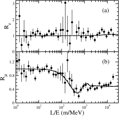
Figure 1: Data and fits for the Super-K atmospheric experiment: (a) electron-like and (b) muon-like events. Data is represented by points. Fit 1 and fit 2, which is not distinguishable, yield the solid line; solution SS, the dashed-dotted line, is only barely distinguishable.

parameter$\backslash$fit	SS	#1	#2
$\chi^{2}_{dof}$	—	1.19	1.21
$\theta_{12}$	$0.54\pm 0.05$	0.48	0.49
$\theta_{13}$	$\leq 0.13$	0.12	$-.04$
$\theta_{23}$	$0.79\pm 0.06$	0.81	0.71
$\Delta m^{2}_{21}\times 10^{-5}({\rm eV})^{2}$	$8.3\pm 0.4$	7.6	7.7
$\Delta m^{2}_{32}\times 10^{-3}({\rm eV})^{2}$	$2.4\pm 0.3$	2.6	2.6
$N_{atm}$	—	1.00	1.00
$N_{Kam}$	—	1.00	1.00

Table 2: The value of $\chi^{2}_{dof}$ and the parameters for the standard solution (SS) and for the two local minima found here.

We fit the mixing angles, the mass squared differences, $N_{atm}$ and $N_{Kam}$ to the quantities in Table 1 and to the $L/E$ dependence of ${\cal R}_{e}$ and ${\cal R}_{\mu}$ pictured in Fig. 1 by minimizing chi-squared per degree of freedom, $\chi^{2}_{dof}$. In Fig. 2 we present $\Delta\chi^{2}=:\chi^{2}_{dof}-\chi^{2}_{min}$ as a function of $\theta_{13}$, where for each value of $\theta_{13}$ we have minimized with respect to the other parameters. The results are not symmetric about $\theta_{13}=0$, and we find two minima. The absolute minimum is at $\theta_{13}=0.12$, and there is a second local minimum at $\theta_{13}=-0.04$. This asymmetry and the existence of the second local minimum would not exist if the commonly used factorization approximation to the oscillation probabilities were employed, as this gives oscillation probabilities that are functions of $\sin^{2}\theta_{13}$.

In Table 2 we present the oscillation parameters for the two minima which we have found and also for a solution where $\Delta m^{2}_{21}$, $\theta_{12}$, and $\theta_{13}$ are taken from the analysis of Ref. bahc , and $\Delta m^{2}_{32}$ and $\theta_{23}$ are taken from Ref. gonz . We term this latter solution the “standard solution” (SS). We see that the parameters we find, particularly for the absolute minimum with $\theta_{13}>0$, are reasonably consistent with those for the standard solution. We remind the reader that we built the model model not to extract precise values of the oscillation parameters, but to examine features of neutrino oscillation phenomenology in a semi-quantitative way. Here, we use the model to investigate the role of the negative $\theta_{13}$ region.

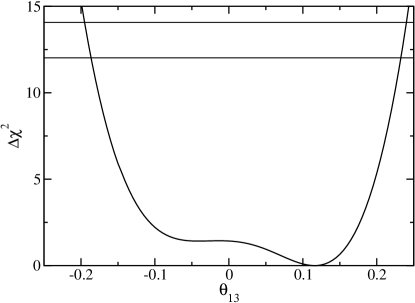
Figure 2: The value of $\Delta\chi^{2}$ for a fixed value of $\theta_{13}$ with all other parameters varied. The horizontal lines indicate the 90% and 95% CL.

Experiment	Data	SS	#1	#2
Chlorine	$.337\pm.065$	.451	.448	.454
Gallium	$.550\pm.048$	.578	.615	.623
SNO	$.348\pm.075$	.395	.371	.378
SNO-salt	$.306\pm.035$	.395	.371	.378
CHOOZ	$>.96$	.98	.96	.99
KamLAND	$.686\pm.006$	.577	.661	.670
K2K	$.55\pm.19$	.60	.56	.57

Table 3: The experimental results and the predictions for each from the models whose parameters are given in Table 2.

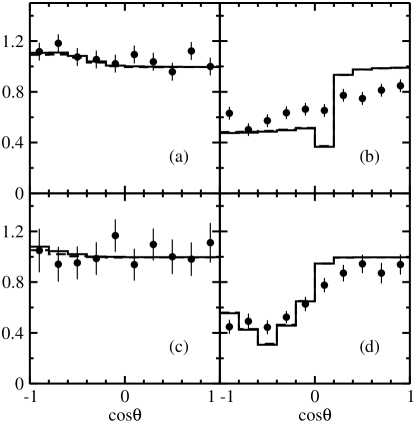
Figure 3: Zenith-angle distributions for atmospheric Super-K experiment. Points represent the data, and the solid line shows the results of Fit 1. (a) Sub-GeV electron-like. (b) Sub-GeV muon-like. (c) Multi-GeV electron-like. (d) Multi-GeV muon-like and PC events.

In Table 3 we compare the data with the results of the fits, and in Fig. 1 we depict the $L/E$ dependence of each fit as compared to the atmospheric data. In Fig. 1 curves are drawn for all three solutions. However, the results are sufficiently similar that the individual curves cannot be distinguished. The model treatment of the atmospheric data is thus seen to be quite comparable to a full analysis. The resulting fits to the data in Table 3 are also seen to be reasonable.

In order to further demonstrate that our results are reasonable, we calculate the zenith-angle dependence of the atmospheric data. Using the energies defined for the various classes of neutrino events in atm , we determine $\mathcal{R}_{e}$ and $\mathcal{R}_{\mu}$ for 10 bins ranging from downward going ($\cos{\theta}=1$) to upward going ($\cos{\theta}=-1$) neutrinos. We also allow for a simple, but more realistic, energy dependence for $n(E)$, taken from honda ; additionally, we introduce some overlap of the bins. We compare our results for the azimuthal dependence of the neutrinos to the dependence of the observed recoil electrons seen at Super-K, normalized to their no-oscillation Monte Carlo simulation, in Fig. 3. Though we do not model the recoil electron, there is a strong correlation between the two processes for the high-energy events. The results are encouraging. For the lower energies, all the solutions produce little electron neutrino oscillations as indicated by the data. However, there is a visible low-energy muon neutrino oscillation which is larger in the theory than in the data. An improved model of the atmospheric data is required to better understand this. Most importantly, the high-energy muon zenith-angle data is qualitatively similar to the results given by our model.

In summary, within the model developed in Ref. model of the neutrino oscillation data, we find that the region $\theta_{13}<0$ plays an important role in understanding the oscillation parameters for three-neutrino oscillations. As oscillation probabilities for negative and positive values of $\theta_{13}$ are not simply related, the analysis cannot be performed in terms of $\sin^{2}\theta_{13}$. The work presented here is intended to motivate a more thorough and careful examination of the $\theta_{13}<0$ region of the parameter space.

- [1] Particle Data Group, Phys. Lett. B592 (2004).
- [2] J. Gluza and M. Zralek, Phys. Lett. B517, 158 (2001).
- [3] D. C. Latimer and D. J. Ernst, nucl-th/0405073.
- [4] B. T. Cleveland, et al., Astrophys. J. 496, 505 (1998).
- [5] J. N. Abdurashitov, et al., Phys. Rev. C 60, 055801 (1999); J. Exp. Theor. Phys. 95, 181 (2002); W. Hampel, et al., Phys. Lett. B447, 127 (1999); M. Altmann, et al., Phys. Lett. B490, 16 (2000).
- [6] Y. Fukuda, Phys. Rev. Lett. 77, 1683 (1996), 81, 1158 (1998), 82, 2430 (1999); 86, 5651 (2001); Q. R. Ahmad, et al., Phys. Rev. Lett. 87, 071301 (2001); Phys. Rev. Lett. 89, 011301 (2002);
- [7] S. N. Ahmed, Phys. Rev. Lett. 92, 181301 (2004).
- [8] M. Apollonio, et al., Phys. Lett. B 420, 397 (1998); B466, 415 (1999); Eur. Phys. J. C 27, 331 (2003).
- [9] K. Eguchi, et al., Phys. Rev. Lett. 90, 021802 (2003); T. Araki, hep-ex/0406035.
- [10] Y. Fukuda, et al., Phys. Lett. B335, 237 (1994); B433, 9 (1998); B436, 33 (1998); Phys. Rev. Lett. 81, 1562 (1998); Phys. Lett. B436, 33 (1998); Phys. Rev. Lett. 82, 2644 (1999); 86, 5651 (2001); Y. Ashie, et al., Phys. Rev. Lett. 93, 101801 (2004).
- [11] M. H. Ahn, et al., Phys. Rev. Lett. 90, 041801 (2003).
- [12] C. Athanassopoulos, et al., Phys. Rev. Lett. 77, 3082 (1996); Phys. Rev. C 54, 2685 (1996); Phys. Rev. Lett. 81,1774 (1998); Phys. Rev. C 58, (2489); A. Aguilar et al., Phys. Rev. D 64, 112007 (2001).
- [13] B. Armbruster, et al., Phys. Rev. D 65, 112001 (2002).
- [14] J. N. Bahcall, M. H. Pinsonneault, and S. Basu, Astrophys. J. 555, 990 (2001).
- [15] L. Wolfenstein, Phys. Rev. D 17, 2369 (1978); S. P. Mikheyev and A. Yu Smirnov, Sov. J. Nucl. Phys. 42, 913 (1985).
- [16] D. C. Latimer and D. J. Ernst, in preparation.
- [17] J. N. Bahcall, M. C. Gonzalez-Garcia, and C. Peña Garay, JHEP 0408, 016 (2004)
- [18] M. C. Gonzalez-Garcia and M. Maltoni, to appear in 5th Workshop on Neutrino Ociallations and their Origins (NOON2004), Tokyo, Japan, February 2004. hep-ph/0406056.
- [19] M. C. Gonzalez-Garcia and Y. Nir, Rev. Mod. Phys. 75, 345 (2003).
- [20] A. Gouvêa and C. Peña-Garay, hep-ph/0406301.
- [21] S. M. Bilenky, C. Giunti, and W. Grimus, Prog. Part. Nucl. Phys. 43, 1 (1999).
- [22] M. Honda, T. Kajita, K. Kasahara, and S. Midorikawa, Phys. Rev. D 52, 4985 (1995).