Quark coalescence into opposite parity baryon states

Abstract

The production rate of negative parity baryons was found to be much weaker than that of positive states in RHIC experiments. In the present paper we show that this suppression is a simple consequence of the coalescence dynamics of hadronization.

1 Preludium

The speculations on the nature of quark gluon plasma (QGP) has a long history. It was assumed, that due to the large momenta of quarks and gluons in the plasma phase, the interaction between them become negligible small as a consequence of the running coupling constant. This idea of non interacting massless quarks and gluons in a big bag was used by many authors, e.g. the authors listed in Ref. [1].

However, it became clear soon, that conditions necessary to create such a plasma, as depicted in the cartoon (see Fig. 1), cannot be fulfilled in the heavy ion collisions. The collision time is too short, the volume is too small, the temperature is too low to produce this massless QGP. Therefore the investigations developed in the direction, that what is the structure of the matter produced in the heavy ion reactions. (Unfortunately strongly different structures were also named ”quark gluon plasma”. Thus it is high time to use different names for the different, well defined matter structures.)

One of the most important qualifiers to characterize the matter is the dominant degree of freedom. In the original quark gluon plasma investigations the dominant degrees of freedom were the massless quarks and gluons. With the realization, that at the hadronization stage these quarks interact strongly, the constituent quarks, which have large effective mass, were considered the dominant degrees of freedom. This development brought up the idea of coalescence hadronization [2].

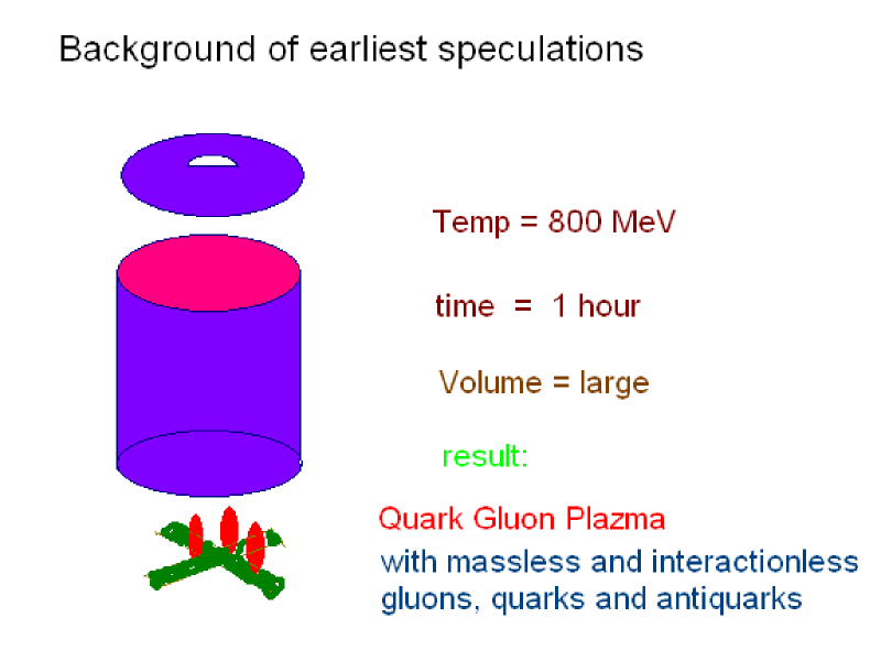
Fig. 1.: Visualization of the cooking of quark-gluon soup.

Here it is important to emphasize, that two different coalescence hadronization models were developed.

In our model it was assumed, that during hadronization both the quark numbers and antiquark numbers are conserved [2], leading to the simple and transparent quark counting scenario [3, 4]. In the other case one assumes, that new quark - antiquark pairs are created during the hadronization, and only the net quark numbers are conserved [5].

After these original calculations a large number of new publications, dealing with different observation, confirmed the validity of the coalescence model [6, 7, 8, 9, 10]. In the present paper we show that the most recently found suppression of negative parity baryons is also the direct consequence of coalescence hadronization.

2 Introduction

In the early rehadronization studies the main efforts were concentrated on the production probabilities of the lowest baryon multiplets. The structure of the particles belonging to these multiplets were similar: they all belonged to the spherical symmetric $l=0$ orbital angular momentum state. Experimentally also these low lying angular momentum states were observed. Presently, however, an opposite parity state ($\Lambda(1520)$) also has been observed experimentally [11, 12].

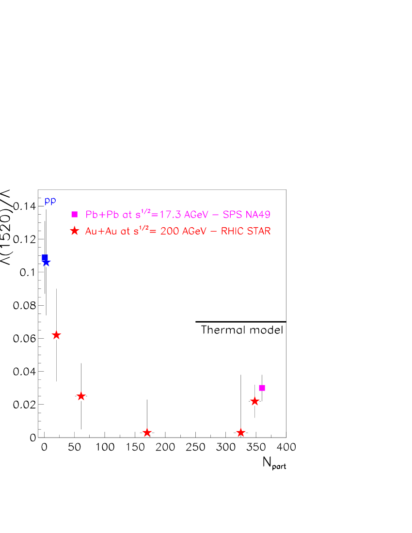
Fig. 2.: The $\Lambda(1520)/\Lambda$ ratios measured by NA49 (squares) [11], and STAR (stars) [12]. The horizontal line corresponds to a thermal model [13].

Figure 2 displays a compilation of experimental values of $\Lambda(1520)/\Lambda$ ratio from NA49 [11] and STAR [12] together with the result of a thermal model from Ref. [13]. The figure clearly shows the suppression of this ratio in central and semi-central $AuAu$ collisions, where quark coalescence is expected.

In the present paper we repeat our earlier calculations of coalescence of constituent quarks into baryons [2], but now with the inclusion of opposite parity final states. We will demonstrate the effect of the symmetry of the internal wave function of the produced hadrons on the transition rates.

In our model the structure of a single hadronization step is assumed as follows. In the initial state we have a diquark (${\cal N}$) interacting with the background quark system. Due to this interaction the background quarks form a screening cluster (${\cal A}$). An incident strange quark (${\cal P}$) will pass this cluster picking up the diquark, forming a new baryon ${\Lambda}$, which leaves the reaction zone.

For easier understanding we demonstrate this process with an educational model and calculate nuclear cross section for the proton - deuteron pick up reaction: $p+(A+n)\rightarrow d+A$ [14]. Here the “proton” plays the role of the strange quark, the “neutron” is the picked up diquark, and the “deuteron” is the final state baryon, $\Lambda$. Real deuteron has only s-wave and d-wave wave-function component, the p-wave state is missing. Since color forces are much stronger than the realistic nuclear forces between real proton and neutron, p-wave baryons exist in the nature. Thus we allow the existence of the p-wave deuteron in our educational model.

3 Simple quantum mechanical model for coalescence process

Considering an incident proton with momentum ${\bf k_{p}}$ in the center of mass of the $p$ and $(A+n)$ system, the pick-up cross section can be written as follows [14]:

$$\sigma_{p+(A+n)\rightarrow d+A}({\bf k_{p},k_{d}})=\frac{v_{d}}{v_{p}}|g_{p+(A+n)\rightarrow d+A}({\bf k_{p},k_{d}})|^{2}\ .$$ (1)

Here the matrix element of the coalescence reaction is determined by the interaction potential $V_{np}({\bf r_{n}-r_{p}})$ and can be calculated as

$$g_{p+(A+n)\rightarrow d+A}({\bf k_{p},k_{d}}) = -\frac{M_{d}}{2\pi\hbar^{2}}\int\displaystyle{\int}\Psi_{A}^{*}({\bf\xi})\phi_{d,l_{d}}^{*}({\bf r_{n}-r_{p}})\cdot e^{-i{\bf k_{d}\cdot(r_{n}+r_{p})/2}}\cdot$$ (2)

$$\hskip 14.22636pt\cdot\ V_{np}({\bf r_{n}-r_{p}}).\Psi_{A,n}({\bf\xi,r_{n}})\cdot e^{i{\bf k_{p}\cdot r_{p}}}d{\bf\xi}d{\bf r_{n}}d{\bf r_{p}}\ ,$$

The internal wave function of the produced final particle is noted by $\phi_{d,l_{d}}$, where $l_{d}$ is the internal angular momentum of the captured neutron in the ground and excited state of “deuteron”. After integration over variable $\xi$ one obtains

$$g_{p+(A+n)\rightarrow d+A}({\bf k_{p},k_{d}}) = -\frac{M_{d}}{2\pi\hbar^{2}}\displaystyle{\int}\phi_{d,l_{d}}^{*}({\bf r_{n}-r_{p}})\cdot e^{-i{\bf k_{d}\cdot(r_{n}+r_{p})/2}}$$ (3)

$$\hskip 14.22636pt\cdot\ V_{np}({\bf r_{n}-r_{p}})\cdot\psi_{n}({\bf r_{n}})\cdot e^{i{\bf k_{p}\cdot r_{p}}}d{\bf r_{n}}d{\bf r_{p}}\ .$$

Here the wave function of the neutron bound to the nucleus $A$ is defined as

$$\psi_{n}({\bf r_{n}})=\displaystyle{\int}\Psi_{A}^{*}({\bf\xi})*\Psi_{A,n}({\bf\xi,r_{n}})d{\bf\xi}$$ (4)

Introducing new spatial variables $R=(r_{n}+r_{p})/2$,  $r=(r_{n}-r_{p})$ and the momentum difference ${\bf K}={\bf k_{p}-k_{d}}$, we arrive to the expression:

$$g_{p+(A+n)\rightarrow d+A}({\bf k_{p},k_{d}}) = -\frac{M_{d}}{2\pi\hbar^{2}}\displaystyle{\int}\displaystyle{\int}F_{d,l_{d}}^{*}({\bf k_{p},r})\cdot G_{n}({\bf K,R+r/2})d{\bf r}d{\bf R}\ \ .\ \$$ (5)

In the following we calculate this matrix element in eq.(5), where the “deuteron” and “neutron” parts are given as

$$F_{d,l_{d}}({\bf k_{p},r}) = \phi_{d,l_{d}}^{*}({\bf r})\cdot V_{np}({\bf r})e^{-i{\bf k_{p}\cdot r/2}}$$

$$G_{n}({\bf K,R+r/2}) = \psi_{n}({\bf R+r/2})e^{i{\bf K\cdot R}}$$ (6)

3.1 Deuteron part

We shall assume that the interaction potential between the incoming “proton” (diquark) and the picked up “neutron” (quark) has the form:

$$V_{np}(r)=\left\{\begin{array}[]{cc}V_{inside}&\mbox{for $r<a$}\\ V_{outside}&\mbox{for $r\geq a$}\ \ ,\end{array}\right.$$ (7)

together with the assumption of $V_{outside}\longrightarrow\infty$. The interaction range $a$ is expected to be in the order of baryon size.

Fig. 3.: Radial wave functions of baryon with $l_{d}=0$ and $l_{d}=1$ states at $a=0.7$ fm.

The radial wave function of the deuteron will be approximated by the spherical Bessel functions as

$$u_{d,0}(r)=n_{d,0}\cdot j_{0}((r/a)\cdot 3.14)$$

$$u_{d,1}(r)=n_{d,1}\cdot j_{1}((r/a)\cdot 4.50)\ ,$$ (8)

where we used the well known spherical Bessel functions,

$$j_{0}(z)=sin(z)/z$$

$$j_{1}(z)=sin(z)/z^{2}-cos(z)/z\ .$$ (9)

After the first zero of the Bessel functions, $x_{0}=3.14$ and $x_{1}=4.50$, we shall assume the radial wave function to be identically zero.

Furthermore, the normalization equations

$$\int_{0}^{\infty}u_{d,l_{d}}(r)^{2}r^{2}dr=1$$ (10)

can be satisfied by introducing $n_{d,0}=0.22525\cdot a^{3/2}$ and $n_{d,1}=0.15327\cdot a^{3/2}$ normalization factors.

The complete deuteron wave function can be written as

$$\phi_{d,l_{d}}({\bf r})=Y_{l_{d},0}(\Theta,\phi)\cdot u_{d,l_{d}}(r)$$ (11)

With these notations the ”deuteron part” of the matrix element has the form

$$F_{d,l_{d}}(k_{p},r)=\phi_{d,l_{d}}({\bf r})\cdot V_{np}(r)\cdot e^{-i{\bf k_{p}r}/2}\\$$

3.2 Neutron part

The neutron wave function, which is assumed to model quark wave function inside the deconfined region, will be approximated by a Gaussian:

$$\psi_{n}({\bf R+r/2})=N\cdot\exp\left[-\frac{1}{s^{2}}({\bf R+r/2})^{2}\right]$$ (12)

with normalization factor

$$N=\frac{2}{\pi^{1/4}\cdot s^{3/2}}\ \ .$$ (13)

The Taylor expansion of this wave function around r = 0 is written as

$$\psi({\bf R+r/2}) = \psi({\bf R})+\nabla\psi({\bf R})\cdot{\bf(r/2)}+\triangle\psi({\bf R})\cdot{\bf(r/2)^{2}}+...$$ (14)

Substituting the Gaussian wave function from eq.(12) into eq.(14) one obtains

$$\psi({\bf R+r/2})\ \ =\ \ N\cdot e^{-\frac{1}{s^{2}}\cdot{\bf R}^{2}}\cdot$$

$$\hskip 14.22636pt\left[1+\frac{-2}{s^{2}}\cdot{\bf R\cdot(r/2)}+\frac{2}{s^{4}}\cdot(2\cdot(x^{2}.X^{2}+y^{2}.Y^{2}+z^{2}.Z^{2})-s^{2}.r^{2})/4\right]\ \ .\ \ \ \$$ (15)

Let us insert this expression into eq.(5)

$$\ \ g_{p+(A+n)\rightarrow d+A}({\bf k_{p},K})=-\frac{M_{d}}{2\pi\hbar^{2}}\displaystyle{\int}\displaystyle{\int}F_{d,l_{d}}^{*}({\bf k_{p},r})\ \cdot\ N\cdot e^{-{\bf R}^{2}}\cdot e^{i{\bf K\cdot R}}$$

$$\hskip 14.22636pt\cdot\left(1+\frac{-2}{s^{2}}*{\bf R\cdot r}+\frac{2}{s^{4}}*(2*(x^{2}.X^{2}+y^{2}.Y^{2}+z^{2}.Z^{2})-s^{2}.r^{2})\right)d{\bf r}d{\bf R}\ \ .\ \ \$$ (16)

3.3 Space integral of the deuteron part

Let us calculate the following integral:

$$I_{l_{d}}({\bf k_{p}}) = -\frac{M_{d}}{2\pi\hbar^{2}}\int F_{d,l_{d}}^{*}({\bf k_{p},r})d{\bf r}$$ (17)

$$= -\frac{M_{d}}{2\pi\hbar^{2}}\int Y_{l_{d},0}(\theta_{r},\phi_{r})\cdot u_{l_{d}}(r)V_{np}(r)\cdot e^{-i{\bf k_{p}r}/2}d\Omega_{r}r^{2}dr$$

Inserting the Raighley expansion into eq.(17)

$$I_{l_{d}}({\bf k_{p}}) = -\frac{M_{d}}{2\pi\hbar^{2}}\displaystyle{\int}Y_{l_{d},0}(\theta_{r},\phi_{r})\cdot u_{d,l_{d}}(r)V_{np}(r)$$ (18)

$$\cdot\sum_{l=0}^{\infty}\sum_{m=-l}^{l}i^{l}j_{l}(k_{p}r/2)Y_{l,m}^{*}(\theta_{r},\phi_{r})\cdot Y_{l,m}(\theta_{p},\phi_{p})d\Omega_{r}r^{2}dr\ \ ,\ \$$

and using the orthogonality relation

$$\int Y_{l,m}^{*}(\theta_{r},\phi_{r})\cdot Y_{k,n}(\theta_{r},\phi_{r})d\Omega_{r}=\delta_{l,k}.\delta_{m,n}\ \ ,\ \$$ (19)

we arrive to the following expression:

$$I_{l_{d}}({\bf k_{p}}) = -i^{l_{d}}\cdot\frac{M_{d}}{2\pi\hbar^{2}}\int u_{d,l_{d}}(r)V_{np}(r)j_{l_{d}}(k_{p}r/2)\cdot r^{2}dr\cdot Y_{l_{d},0}(\theta_{p},\phi_{p})\ \ .$$ (20)

This integral has to be multiplied by the first term of the Taylor expansion of the ”neutron part”:

$$B_{n}({\bf K}) = \int N\cdot e^{-(R/s)^{2}}\cdot Y_{0,0}(\Omega_{R})\cdot e^{i{\bf K.R}}d\Omega_{R}R^{2}dR$$ (21)

$$= N\cdot\int e^{-(R/s)^{2}}\cdot j_{0}(K\,R)R^{2}dR$$

Thus the complete matrix element in first order approximation is given as:

$$g_{p+(A+n)\rightarrow d+A}({\bf k_{p},K})=I_{l_{d}}({\bf k_{p}})*B_{n}({\bf K})$$ (22)

Choosing the Z axis in the direction of ${\bf k_{p}}$, we have $\theta=0,\phi=0$, and thus

$$I_{l_{d}}(k_{p}) = -i^{l_{d}}[\frac{2l_{d}+1}{4\pi}]^{1/2}\cdot\frac{M_{d}}{2\pi\hbar^{2}}\displaystyle{\int}u_{d,l_{d}}(r)V_{np}(r)j_{l_{d}}(k_{p}r/2)\cdot r^{2}dr$$ (23)

Thus the production rate, $A_{l_{d}}$ depends on the bombarding momentum, $k_{p}$ and it is determined as

$$A_{l_{d}}(k_{p})={\cal C}\cdot|I_{l_{d}}(k_{p})|^{2}\ \ ,$$ (24)

where ${\cal C}$ is a constant, independent on $l_{d}$.

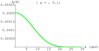
Fig. 4.: Space integrated matrix element squared $A_{0}(k)$ in eq.(24) at $a=0.3$ fm.

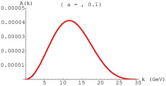
Fig. 5.: Space integrated matrix element squared $A_{1}(k)$ in eq.(24) at $a=0.3$ fm.

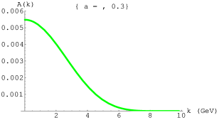
Fig. 6.: Space integrated matrix element squared $A_{0}(k)$ in eq.(24) at $a=0.3$ fm.

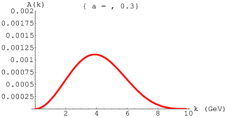
Fig. 7.: Space integrated matrix element squared $A_{1}(k)$ in eq.(24) at $a=0.3$ fm.

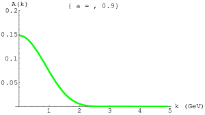
Fig. 8.: Space integrated matrix element squared $A_{0}(k)$ in eq.(24) at $a=0.9$ fm.

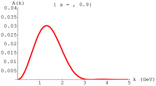
Fig. 9.: Space integrated matrix element squared $A_{1}(k)$ in eq.(24) at $a=0.9$ fm.

4 Numerical results

We calculated the production rates $A_{0}$ and $A_{1}$ at interaction ranges $a=0.1,\ 0.3,\ 0.9$. The obtained results are displayed in Figs. 4-9.

The total transition rate, $R_{l}$, is obtained by the integration of $A_{l_{d}}(k_{p})$, weighted by the distribution function $f(k_{p})$:

$$R_{l_{d}}=\int_{0}^{\infty}f(k_{p})\cdot A_{l_{d}}(k_{p})dk_{p}\ \ .$$ (25)

Here $f(k_{p})$ is the momentum of the proton relative to the center of mass of the neutron and screening cluster system. For the present numerical calculations we used a Boltzmann function:

$$f(k_{p})=Exp[-k_{p}/T]$$ (26)

(We mention here that for coalescence within parton shower [15] a narrower distribution function should be used.)

The obtained $R_{0}$, $R_{1}$ production rates can be connected to the production rates of $\Lambda(1114)$ and $\Lambda(1520)$, respectively. Assuming a fast hadronization at the critical temperature, $T_{c}$, one can directly compare the obtained $R_{1}/R_{0}$ ratios to the measured $\Lambda(1520)/\Lambda(1114)$ ratio. Fig. 10 displays our result for $R_{1}/R_{0}$ as a function of the interaction range, $a$ (solid line). The shaded area indicates the experimental result $\Lambda(1520)/\Lambda(1114)=0.022\pm 0.01$ measured by the STAR at RHIC [12]. The dashed line shows the calculated thermal ratio [13]. From Fig.10 one can conclude that the $R_{1}/R_{0}$ ratio calculated in our coalescence model using the interaction range $a=0.8-1.0$ fm is consistent with the experimental data.

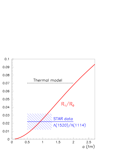
Fig. 10.: Suppression factor as a function of interaction range, $a$.

5 Summary

It is an inherent property of the coalescence rehadronization model that the production of the $\Lambda(1520,J^{P}=\frac{3}{2}^{-})$ baryon is strongly suppressed in comparison to the production of $\Lambda(1114,J^{P}=\frac{1}{2}^{+})$.

This is due to the fact that in $\Lambda(1520)$ the orbital angular momentum of one of the constituent quark differs by one unit from that of the corresponding quark in $\Lambda(1114)$. The strength of the suppression depends on the length of interaction.

From the above consideration one may conclude, that i) in the STAR Au+Au reaction a sort of quark matter was formed, meaning that in this case the dominant degrees of freedom are the constituent quarks, and ii) such matter was not formed in the $p+p$ reaction or in peripheral $Au+Au$ reactions.

One has to mention, however, that it is somewhat surprising, that in the SPS $Pb+Pb$ reaction at $\sqrt{s}=17.3$ AGeV such a suppression also exists.

References

-
[1]
J. Rafelski and B. Müller:
Strangeness Production in the Quark-Gluon Plasma,
Phys. Rev. Lett. 48, 1066 (1982);
T.S. Biró and J. Zimányi: Quarkochemistry in relativistic heavy ion collisions, Phys. Lett. B113, 6 (1982);
B. Müller: The Physics of the Quark-Gluon Plasma, Lect. Notes in Phys., 225 (1985);
K. Kajantie and H.I. Miettinen: Temperature measurement of quark-gluon plasma formed in high energy nucleus-nucleus collisions, Z. Phys. C9, 341 (1981);
M. Gyulassy: Formation of a quark-gluon plasma in nuclear collisions, LBL-14512, (1982) - [2] T.S. Biró, P. Lévai, and J. Zimányi, Phys. Lett. B347, 6 (1995); Phys. Rev. C59, 1574 (1999).
- [3] A. Bialas, Phys. Lett. B442, 449 (1998).
- [4] T.S. Biró, T. Csörgő, P. Lévai, and J. Zimányi, Phys. Lett. B472, 243 (2000).
- [5] R.C. Hwa and C.B. Yang, Phys. Rev. C66, 064903 (2002).
- [6] A. Bialas, Phys. Lett. B532, 249 (2002).
- [7] A. Bialas, Phys. Lett. B579, 31 (2004).
- [8] V. Greco, C.M. Ko, P. Lévai, Phys. Rev. Lett. 90, 202302 (2003); Phys. Rev. C 68, 034904 (2003).
- [9] R.J. Fries, B. Müller, C. Nonaka, S.A. Bass, Phys. Rev. Lett. 90, 202303 (2003); Phys. Rev. C68, 044902 (2003).
- [10] D. Molnár, S.A. Voloshin, Phys. Rev. Lett. 91, 092301 (2003); Z.W. Lin, D. Molnar, Phys. Rev. C68, 044901 (2003).
- [11] V. Friese for the NA49 Collaboration, Nucl. Phys. A698, 487 (2002).
- [12] L. Gaudichet for STAR collaboration, nucl-ex/0307013.
- [13] P. Braun-Munziger, D. Magestro, K. Redlich, J. Stachel, Phys. Lett. B518, 41 (2001).
- [14] Rearrangement collision, Section 34., in L.I. Schiff: Quantum Mechanics, Second edition, McGraw Hill, New York, 1955.
- [15] R.C. Hwa, C.B. Yang, nucl-th/0401001.